Ascent trajectory tracking for an air-breathing hypersonic vehicle with guardian maps

Abstract

The emphasis of this article lies in the development of a gain scheduling algorithm for the constant dynamic pressure ascent trajectory. Due to the broad flight envelope and nonlinear characteristics of hypersonic vehicles, a design method of adaptive control based on guardian maps is proposed. Two types of ascent trajectory are considered: acceleration within Scram mode and acceleration across the Ram–Scram mode transition. A velocity-based linear parameter varying model of an air-breathing hypersonic vehicle is established. The gain vector of controller is determined via optimal control theory based on linear quadratic regulator technology with the specified flying qualities. With the iteration of proposed guardian maps approach, the set of controller gain vector within the flight envelope is obtained. The results of nonlinear simulation show that the proposed approach of control system design has the ability to ensure the global stability through the flight envelope and to maintain the flying qualities.

Introduction

In the past decade, there has been a sustaining effort devoted to investigating the dynamic model of air-breathing hypersonic vehicles (AHSV) for simulation and control design purposes. ^{1 –3} Several interesting trade-offs should be taken into consideration for scramjet-powered AHSV. An AHSV with lifting body structure uses lift to counter gravity. It is well known that a rocket launcher tends to maximize its acceleration early in the trajectory for optimization of the fuel consumption. However, for scramjet-powered vehicle, burning too much fuel may cause thermal choking in the combustor or result in unstart, accordingly the maximum acceleration may be limited. Besides, a higher dynamic pressure leads to the static pressure in the combustor and the combustion efficiency. On the contrary, structural considerations restrict the achievable dynamic pressure. Thus, the trajectory design for such hypersonic vehicles is vital for accomplishment of mission. ⁴

The flight dynamics and control approaches for hypersonic vehicles have been summarized by Xu and Shi. ⁵ Control system design for the AHSV is a challenging task stemming from large flight envelope with extreme range of operation conditions, uncertainty, and strong interactions between elastic airframe, propulsion system, and structural dynamics. The major issues include input/output coupling, control saturation, ⁶ dead zone input constraint, ⁷ nonlinear coupling, and model uncertainty. Controller design is crucial in making hypersonic vehicles feasible. Stability, performance, and robustness are three main concerns for the design of guidance and control systems. H_∞ design, μ-synthesis methods, ⁸ linear parameter varying (LPV) technique ^9,10 based on linear control theory by linearizing the model at the operation point have been widely applied. Despite the linear controller may ensure the stability and performance at the design point, some advanced nonlinear control approaches have been studied aiming at investigating the behavior throughout the flight envelope, and the assurance of global stability, ^{11 –13} such as feedback linearization method, ^14,15 dynamic inversion method, ^16,17 adaptive dynamic surface control, ^18,19 neural control, ^20,21 and so on. Apart from the stability, the robustness and flight quality have been taken into consideration in the case of system uncertainty and parameter variation. ²²

However, the nonlinear control approaches demand analytic expression of models and the construction of nonlinear controller is quite complicated. Using the LPV techniques, a nonlinear model can be described based on a set of linear models on trimmed points. Consequently, the controller gain of the nonlinear system can be obtained by synthesizing a sequence of linear time invariable (LTI) controllers. In view of this merit of LPV model, LPV technique is a promising approach to deal with the control design issue for hypersonic vehicles with wide flight envelope and strong uncertainty. There are several approaches used to obtain reliable LPV models, such as Jacobian linearization, state transformation, function substitution, linear fractional transformation, and different types of linearization. ²³ The velocity-based linearization techniques proposed by Leith and Leithead ²⁴ provide very general and soundly based methods for transforming systems into LPV/quasi-LPV form. In contrast to the conventional linearization method, the velocity-based analysis and design framework associate a linear system with every operating point of a nonlinear system, not just the equilibrium operating points. ²⁵

The guardian maps approach as a unifying tool for the study of generalized stability of parameterized families of matrices or polynomials was introduced by Saydy et al. ²⁶ Practical work has been done in the field of stability analysis of parameterized system, for example, exact stability analysis of 2-dimensional systems ²⁷ and robust stability analysis of an interval system. ²⁸ Recently, this approach has been in-depth studied to find controller gains in flight control systems. ^29,30 Unlike the adaptive control design, which may construct a Lyapunov function to adjust the control signal with the variation of parameters, ³¹ guardian maps may confirm the boundary of parameters that ensure the closed-loop stability and guarantee the stability and flight quality of the switching procedure of the control parameters. Any suitable control design methods may be used by means of the guardian maps approach. This method enables to automatically search for the design point and ensures the system stability within the flight envelope, which precedes the traditional gain scheduling control design method. As for the system of higher dimensions, this approach exhibits inefficiency in parameters searching process and the results are very sensitive to the selected initial values.

The focus of this work is on the control design and simulation for tracking ascent trajectory for constant dynamic pressure of scramjet-powered AHSV. First, an AHSV model with dual-mode scramjet propulsion system is introduced. Next, two types of optimal ascent trajectory are discussed, target cruise point of which is optimized for the minimal fuel consumption per range. In “Tracking control with guardian maps” section, some preliminaries about guardian maps and synthesis procedure for constant dynamic ascent phase are presented. Then, a velocity-based LPV model of AHSV is established and an adaptive linear quadratic regulator (LQR) controller design method for the full trajectory is proposed. Afterward, the simulation and analysis of the designed controller for the optimal ascent trajectory are presented. The novelty of this article lies in that the controller gains can be automatically obtained as long as an initial point is selected, meanwhile, the flying quality along the profile can be guaranteed.

Model description

The AHSV for this work is a generic wave rider as shown in Figure 1. The first principle model of a scramjet-powered AHSV was developed as an attempt to extend earlier work done by Bolender and Doman, ³² which includes parameterized geometry generation, dual-mode scramjet performance analysis, and aerodynamic analysis based on finite panels method. ³³

Figure 1.

Vehicle configuration.

Considering the model for the longitudinal dynamics of an AHSV, the point mass equations of motion for 3 degree of freedom (3DOF) rigid vehicle over a rotating spherical earth are given as follows

$\dot{V}=\frac{T\text{cos}\alpha -D}{m}-g\text{sin}\gamma$

1

$\dot{\gamma }=\frac{T\text{sin}\alpha +L}{mV}+\left(\frac{V}{R_E+h}-\frac{g}{V}\right)\text{cos}\gamma$

2

$\dot{q}=\frac{M}{I_{yy}}$

3

$\dot{h}=V\text{sin}\gamma$

4

$\dot{r}=V\frac{R_E}{R_E+h}\text{cos}\gamma$

5

$\dot{\theta }=q$

6

$\dot{\alpha }=q-\dot{\gamma }$

7

$\dot{m}=-{\dot{m}}_f$

8

where R _E denotes the mean radius of the earth, g denotes the local acceleration of gravity, m,Iyy denotes the mass and moment of inertia about y-axis. L,T,D,M represent the lift, thrust, drag, and pitching moment, respectively. Vehicle states include velocity V, angle of attack α, altitude h, pitch rate q, pitch angle θ, and flight path angle γ. The vehicle has two control inputs: the deflection of a rearward situated elevator δ _e and stoichiometric normalized fuel equivalence ratio ϕ. The force and moment acting on the vehicle can be formulated as ³³

$\begin{array}{l}L=\overline{q}{S}_{\text{ref}}{C}_L(\alpha ,{\delta }_e,Ma,\varphi )\\ D=\overline{q}{S}_{\text{ref}}{C}_D(\alpha ,{\delta }_e,Ma,\varphi )\\ T=\overline{q}{S}_{\text{cap}}{C}_T(\alpha ,Ma,\varphi )\\ M=\overline{q}{S}_{\text{ref}}{l}_{\text{ref}}{C}_m(\alpha ,{\delta }_e,Ma,\varphi )+z_{T}T\end{array}$

9

where $\overline{q}$ denotes the dynamic pressure.

Cruise condition

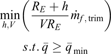
The optimal cruise condition is chosen to be the minimal fuel consumption per range, which is the target flight condition for the ascent trajectory. The objective function for selecting optimal cruise condition is as follows

$J={\dot{m}}_{f,\text{trim}}\frac{(R_e+h)}{V{R}_e}$

10

where ${\dot{m}}_{f,\text{trim}}$ is the fuel mass rate at the trimmed flight condition for given V, h. The lift drag ratio L/D is the major parameter for determining optimal cruise condition.

Meanwhile, the dynamic pressure should not be such low for the sake of the performance of scramjet propulsion system. Thus, the optimal problem can be formulated as

$\begin{array}{c}{\displaystyle \underset{h,V}{\text{min}}}\left(\frac{R_E+h}{V{R}_E}{\dot{m}}_{f,\text{trim}}\right)\\ s\mathrm{.}t\mathrm{.}\overline{q}\ge {\overline{q}}_{\text{min}}\end{array}$

Optimal ascent trajectory for constant dynamic pressure

Trajectory optimization of scramjet-powered AHSV is a challenging task because the performance of the propulsion system is highly sensitive to flight path. An AHSV must climb along a near-minimum fuel trajectory for maximizing its payload capability. The restriction of flying at constant dynamic pressure allows us to determine altitude as a function of Mach number. Differentiating the dynamic pressure with respect to altitude, for $\dot{\overline{q}}=0$

$\frac{dV}{dh}=-\frac{V}{2\rho }\frac{d\rho }{dh}$

11

If we take the acceleration as a design variable, then the equation can be rewritten as

$\dot{V}=a$

12

$\dot{\gamma }=\frac{a}{V\text{cos}\gamma }\left[\frac{d^{2}h}{d{V}^2}a+\left(\frac{da}{dV}-\frac{a}{V}\right)\frac{dh}{dV}\right]$

13

$\dot{h}=\frac{dh}{dV}a$

14

$\dot{r}=V\frac{R}{R+h}\text{cos}\gamma$

15

$\dot{m}=-{\dot{m}}_f$

16

In the present study, the reference optimal ascent trajectory is generated offline using nonlinear programming (NLP) method. Minimum fuel ascent trajectory for constant dynamic ascent phase was solved using sequential quadratic programming technique. The objective for the trajectory is to minimize the total fuel consumption while ascent phase, or alternatively, maximize the orbit mass.

Maximum acceleration

One of the main issues for the scramjet-powered AHSV is the operational mode of the propulsion system along the trajectory, known as Ram mode and Scram mode, which depends on the flight conditions and the temperature increased in the burner. The transition condition of these two modes was investigated in detail by Torrez et al., ³⁴ which indicates that the flow states at the entrance of isolator (also exit of inlet), mainly the Mach number and static pressure, along with the temperature added in the burner are crucial for determination of the operation mode of propulsion system.

The flow within the inlet is assumed to be isentropic, that is, the stagnation temperature is unchanging. The mode of scramjet is related to the stagnation temperature at the entrance of isolator and the total heat release within the burner, which related to the fuel equivalence ratio. The boundary of fuel equivalence ratio is approximated as

${\varphi }^{*}=0.1379M{a}_i+0.0003919T_t-0.429$

17

where Ma_i donates the Mach number at the entrance of isolator, T_t donates the stagnation temperature of freestream.

The proposed method for analysis of isolator burner interaction is well discussed by Heiser and Pratt, ³⁵ which is a simplified version of Michigan-Air Force Scramjet In Vehicle (MASIV). ³⁶ The Ram-to-Scram transition is quantitatively analyzed via the strength of precombustion shocks, ³⁷ which mainly depends on the flow states at the inlet of isolator and the heat added in the burner. Fuel–air equivalence ratio ϕ is defined as the ratio of the fuel-to-oxidizer ratio to the stoichiometric fuel-to-oxidizer ratio, which is equivalent to the “heat release” from the burner.

Figure 2 has shown the maximum acceleration that the vehicle can achieve with respect to velocity. With limitation on the Scram mode, the maximum available acceleration with the same flight condition is deduced by comparing the Ram and Scram mode. As velocity is above 2400 m/s, the propulsion is fully operated at the Scram mode at the maximum acceleration.

Figure 2.

Maximum acceleration with respect to velocity.

Tracking control with guardian maps

Guardian maps

The guardian maps approach as a unifying tool for the study of generalized stability of parameterized families of matrices or polynomials was introduced by Saydy et al. ²⁶ Basically, guardian maps are scalar valued maps defined on the set of n × n matrices or n order polynomials. Consider the stability sets of the form

$S\left(\Omega \right)=\left\{A|\lambda \left(A\right)\subset \Omega ,A\in R^{n\times n}\right\}$

18

where Ω is an open subset of the complex plane of interest and λ(A) denotes the set of eigenvalues of A. Such sets S(Ω) will be referred to as generalized stability sets, all matrices in which have all their eigenvalues in Ω.

Definition I

Let ν denotes the map from the matrix A ∈ R^n×n to C. ³⁸ We say that ν guards S(Ω) or ν is known as guardian map of Ω, if for all $A\in \overline{S}(\Omega )$ , we have

$A\in \partial S\left(\Omega \right)\iff \nu \left(A\right)=0$

19

or ν semiguards S(Ω) or semiguardian map of Ω, if

$\forall A\in \partial S\left(\Omega \right)\Rightarrow \nu \left(A\right)=0$

20

where $\overline{S}$ denotes closure of the set S and ∂S denotes the boundary of the set S.

Some guardian maps are given for classical stability regions ³⁹ (see Figure 3).

Figure 3.

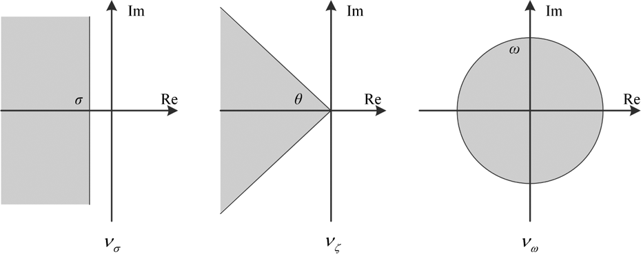
Classic stability sets of guardian maps.

Stability margin: the open σ-shifted half plane region has a corresponding semiguardian map

${\nu }_{\sigma }\left(A\right)=\text{det}\left(A\odot I-\sigma I\odot I\right)\text{det}\left(A-\alpha I\right)$

21

where ⊙ denotes the bialternate product. ²⁶

The conic sector with inner angle 2θ has a corresponding semiguardian map

${\nu }_{\zeta }\left(A\right)=\text{det}\left[A^2\odot I+\left(1-2{\zeta }^2\right)A\odot A\right]\text{det}\left(A\right)$

22

where ζ = cosθ denotes the limiting damping ratio.

Schur stability: for the circle of radius ω > 0 has a corresponding semiguardian map

${\nu }_{\omega }\left(A\right)=\text{det}\left(A\odot A-{\omega }^{2}I\odot I\right)\text{det}\left(A^2-{\omega }^{2}I\right)$

23

Stability characterization

Let $A(r)|r\in U\subset R^k$ be a continuous family of n × n matrices, which depend on the parameter vector r. The bounds of each entry are known in advance.

Theorem I

Let S(Ω) be guarded by the map ν_Ω, ²⁶ the family $A(r)|r\in U$ is stable relative to Ω if and only if

It is nominally stable, that is, $\exists r_0\in U,A(r_0)\in S(\Omega )$ ;

${\nu }_{\Omega }(A(r))$ does not vanish in U, that is, $\forall r\in U,{\nu }_{\Omega }(A(r)){\nu }_{\Omega }(A(r_0))>0$

If the condition 2 is not strictly satisfied, that is, $\forall r\in U,{\nu }_{\Omega }(A(r)){\nu }_{\Omega }(A(r_0))\le 0$ , then ν_Ω is called semiguardian maps.

Corollary I

Let S(Ω) be guarded by the map ν_Ω and consider the matrices family $A(r)|r\in U$ . ³⁹ Then, the set C is defined by

$C=\left\{r|{\nu }_{\Omega }\left[A\left(r\right)\right]=0,r\in R^k\right\}$

24

and divides the parameter space R^k into components C_i that are either stable or unstable relative to Ω.

Velocity-based LPV modeling

Consider a general nonlinear system

$\begin{array}{l}\dot{x}(t)=f(x,u,t)\\ y(t)=g(x,u,t)\end{array}$

25

where f(x,u,t),g(x,u,t) are differentiable nonlinear functions with Lipschitz continuous first derivatives and u(t),y(t),x(t) denotes the input to the plant, the output, and the state, respectively.

A standard approach of obtaining an LPV model is to linearize the nonlinear system at different equilibrium operating points and then map the scheduling variables p(t) to the family of linearization system to achieve an LPV system.

$\begin{array}{l}\Delta \dot{x}\left(t\right)=A\left[p\left(t\right)\right]\Delta x\left(t\right)+B\left[p\left(t\right)\right]\Delta u\left(t\right)\hfill \\ \Delta y\left(t\right)=C\left[p\left(t\right)\right]\Delta x\left(t\right)+D\left[p\left(t\right)\right]\Delta u\left(t\right)\hfill \end{array}$

26

$\begin{array}{l}A\left[p\left(t\right)\right]={\frac{\partial f}{\partial x^T}|}_{x=x_{\text{trim},p},u=u_{\text{trim}, p}}\hfill \\ B\left[p\left(t\right)\right]={\frac{\partial f}{\partial u^T}|}_{x=x_{\text{trim},p},u=u_{\text{trim}, p}}\hfill \end{array}$

where $x_{\text{trim}, p},u_{\text{trim}, p}$ are the trimmed state and control input at the scheduling variable p.

The basic idea of velocity-based linearization is to make a differentiation of equation (25) with respect to time

$\begin{array}{l}\ddot{x}\left(t\right)=A\left[x\left(t\right),u\left(t\right)\right]\dot{x}\left(t\right)+B\left[x\left(t\right),u\left(t\right)\right]\dot{u}\left(t\right)\hfill \\ \dot{y}\left(t\right)=C\left[x\left(t\right),u\left(t\right)\right]\dot{x}\left(t\right)+D\left[x\left(t\right),u\left(t\right)\right]\dot{u}\left(t\right)\hfill \end{array}$

27

where

$\begin{array}{l}A\left[x\left(t\right),u\left(t\right)\right]={\frac{\partial f}{\partial x^T}|}_{x=x(t),u=u(t)}\hfill \\ B\left[x\left(t\right),u\left(t\right)\right]={\frac{\partial f}{\partial u^T}|}_{x=x(t),u=u(t)}\hfill \end{array}$

The velocity-based approach may be regarded as the extend of scheduling variables p^T = [x,u]. What’s more, the states and control inputs of velocity-based LPV model are the differential of states and control inputs, rather than deviation.

With the extension of state $x_e^T=[x,\dot{x},u]$ , the nonlinear system (25) can be reformulated as the following linear form

$\begin{array}{l}\left[\begin{array}{c}\dot{x}\\ \ddot{x}\\ \dot{u}\end{array}\right]=\left[\begin{array}{ccc}0& I& 0\\ 0& A\left(x,u\right)& 0\\ 0& 0& 0\end{array}\right]\left[\begin{array}{c}x\\ \dot{x}\\ u\end{array}\right]+\left[\begin{array}{c}0\\ B\left(x,u\right)\\ I\end{array}\right]\dot{u}\hfill \\ \dot{y}=\left[0C\left(x,u\right)0\right]\left[\begin{array}{c}x\\ \dot{x}\\ u\end{array}\right]\hfill \end{array}$

28

Synthesis procedure

The optimal climb profile for constant dynamic pressure segment of AHSV ascent phase was designed to be tracked, which allows us to formulate vehicle states as functions of velocity. Thus, the gain scheduling parameters can be simplified as one parameter: velocity r = V. Further, the other parameters can be treated as constrains while the closed-loop stability is synthesized.

Let Ω be a stability region of the complex plane and corresponding guardian map ν_Ω, A(r, K) be a closed-loop matrix depending on the parameters r ∈ U. Let K = [K_j] denotes the vector of variable gain of the controller. The objective is to find a controller K such as the closed-loop poles lie in a specific region Ω and determining the boundary of parameters V that guarantee the closed-loop poles remain in Ω as parameters varying.

Gain scheduling algorithm

Step 0: Define the boundary of the parameter $V\in U=[V_{\text{min}},V_{\text{max}}]$ . Set the minimum parameter as the nominal case $V_0=V_{\text{min}}$ . Obtain a controller K₀ designed for the nominal case V₀ ensures nominal stability relative Ω. Set n = 0, denotes the nth iteration.

Step 1: Find the largest stability interval $\left[{\underset{\_}{V}}_n,{\overline{V}}_n\right]$ with constrains of other parameters using a search algorithm for stability interval with specific controller gain Kⁿ.

Step 2: Check out the terminal condition. If the upper boundary of stability interval ${\overline{V}}_n$ is out the U then stop, else set the counter n = n + 1, and the upper boundary of stability interval is set to be nominal case $V_n={\overline{V}}_{n-1}$ , then come to step 3.

Step 3: Redesign a new gain vector Kⁿ to ensure the nominal stability with scheduling variable V_n, then go back to step 1.

Search algorithm for stability interval

Step 0: Given the controller gain Kⁿ and the range of scheduling variable $U=[V_{\text{min}},V_{\text{max}}]$ .

Step 1: Calculate the maximum interval $[\underset{\_}{V},\overline{V}]\subset U$ where the guardian map ν_Ω is not vanished for the closed-loop system with controller Kⁿ, the nominal state $x_V^T=[V,\alpha (V),h(V),q(V),\theta (V)]$ , and the nominal input $u_V^T=[{\delta }_e(V),\varphi (V)]$ .

Step 2: Calculate the stability interval for the other parameters. Take altitude for instance (see Figure 4). For a velocity $V_{n,i}\in [\underset{\_}{V},\overline{V}]$ , use the same method to obtain the stability interval $[\underset{\_}{h}(V_{n,i}),\overline{h}(V_{n,i})]$ , then we can get the upper and lower boundary of altitude with respect to velocity $\overline{h}(V),\underset{\_}{h}(V),V\in [\underset{\_}{V},\overline{V}]$ .

Step 3: For a required altitude stable interval Δh, that for any $|h-h(V)|<\Delta h$ , the stability at region Ω still holds. As result obtained from step 2, we can find the interval of velocity, that $\text{min}[\overline{h}(V)-h(V),h(V)-\underset{\_}{h}(V)]>\Delta h$ is satisfied, then the maximum stability interval of velocity with altitude stability constrains is refined as $[{\underset{\_}{V}}_n,{\overline{V}}_n]\subset [\underset{\_}{V},\overline{V}]$ .

Figure 4.

Illustration of determination of stability interval.

Regulator controller design

In order to obtain the stability region Ω, where the closed-loop poles must lie, one has to map the handling qualities into the complex plane. The commonly considered flying quality criteria are phugoid mode damping ratio ζ_ph, short period mode damping ratio ζ_sp, pitch attitude bandwidth ω_BWθ, phase delay τ_p, path bandwidth ω_BWγ, and Gibson dropback DB. Criteria like damping ratio can be mapped in the complex plane but bandwidth criteria is more difficult to deal with because of the influence of the zeros.

Considering the flying qualities for level 2 from MIL-STD-1797A. ⁴⁰ The parameters are selected as ${\omega }_n\le 6,\eta \ge 0.2,\sigma <-0.36$ . The objective is to find a controller K such as the closed-loop poles lie in the specific region $\Omega (\sigma ,\zeta ,\omega )$ . The stability region is shown in Figure 5.

Figure 5.

Stability region considering flying qualities.

It is desirable to include integral control into the state feedback to eliminate the steady output error. By augmenting the system with the integral error, it is possible to let the LQR routine choose the value of the integral gain automatically.

Let append the output error dynamics to the system (27), to obtain

$\left[\begin{array}{c}\ddot{x}\\ \dot{e}\end{array}\right]=\left[\begin{array}{cc}A\left(x,u\right)& 0\\ -C\left(x,u\right)& 0\end{array}\right]\left[\begin{array}{c}\dot{x}\\ e\end{array}\right]+\left[\begin{array}{c}B\left(x,u\right)\\ 0\end{array}\right]\dot{u}+\left[\begin{array}{c}0\\ I\end{array}\right]\dot{r}$

29

The initial control design problem is to find a linear optimal tracking controller to minimize the cost function

$J=\frac{1}{2}{\displaystyle {\int }_0^{\infty }}\left(e^{T}Qe+u^{T}Ru\right)dt$

30

Meanwhile, the closed-loop poles lie in $\Omega (\sigma ,\zeta ,\omega )$ , where $Q=Q^T\ge 0,R=R^T>0$ . Afterward, the gain vector is determined by the search algorithm for gain of controller.

Search algorithm for gain of controller ³⁸

Step 0: Initialization. $A_{cl}(V_{n+1},K^n)$ denotes a closed-loop matrix depending on the (n + 1)-th iteration scheduling variable $V_{n+1}$ and previous gain vector $K^n=\left\{K_i^n\right\},i=1,\cdots ,k$ of controller. The range of each entry of the gain vector is known in advance $K_i^j\in U_i=[K_{i,\text{min}},K_{i,\text{max}}]$ . Set the tolerance for terminal condition ε. Set j = 0, K^j = Kⁿ.

Step 1: Main loop

For m from 1 to k

Fix all the gains $K_i^j$ of K^j to their current values but $K_m^j$ , then the guardian map $\nu [A_{cl}(V,K^j)]$ is simplified as one parameter $\nu (K_m^j)$

Using theorem I to find the largest stability interval $[{\underset{\_}{k}}_m,{\overline{K}}_m]\subset U_m$ . Set $K_m^{j+1}=({\underset{\_}{k}}_m+{\overline{K}}_m)/2$ .

End

Step 2: Terminal condition. A new gain vector K^j+1 is then obtained. If $|K^j-K^{j+1}|\le \epsilon (1+|K^j|)$ then set Kⁿ⁺¹ = K^j+1 stop, else set j = j + 1, go to step 1.

Gain scheduling algorithm

The series of the controller gain vector is obtained according to the approach described above. As shown in Figure 6, the gain $K_i^n$ designed at the point V_n ensures the stability of region Ω. The upper bound of V_n is ${\overline{V}}_n$ , which is the same point V_n+1 where the gain vector is refined. From the process of searching the new gain $K_i^{n+1}$ , we can conclude that any value from $K_i^n$ to $K_i^{n+1}$ will ensure the stability of region Ω.

Figure 6.

Illustration of gain scheduling algorithm.

The stability interval of V_n+1 is obtained using algorithm described in “Stability region for guardian maps” section, as shown in Figure 6. Different from the switching algorithm for control gain, which will cause first-order discontinuity of control law, two smoothing approaches for gain scheduling are proposed.

First, the control gain is approximated within the covered region (gray region shown in Figure 6) using first-order or higher order polynomials, while the control gain in other region remains the corresponding values (solid line in Figure 6). The other approach is directly using the Lagrangian polynomials to fit the control gain based on the designed points (dotted line in Figure 6).

The first approach will ensure global stability of region Ω via theoretical analysis, yet the gain scheduling algorithm is complicated. On the contrary, the second simplified the gain scheduling process. However, the stability should be inspected. Generally speaking, the global stability for the second approach always remains.

Simulation results

Optimal ascent phase

As discussed in “Model description” section, two general types of ascent trajectories were optimized: acceleration within Scram mode and acceleration across the Ram–Scram mode transition. The target point of ascent trajectory obtained from optimization of cruise condition is 31,401 m and 2625.8 m/s for constant dynamic pressure 50 kPa. The start point is selected as 26,962 m and 1858.6 m/s. The achievable acceleration of these two types ascent profile is different at the lower speed region, which was investigated in “Maximum acceleration” section. The major difference is the earlier period of acceleration phase, which leads to a slow speedup time for Scram mode (see Figure 7).

Figure 7.

Optimal constant dynamic pressure ascent trajectory. (a) Altitude, (b) velocity.

Stability region for guardian maps

Considering the unstable open-loop characteristics of AHSVs, a LQR controller was designed to ensure the closed-loop stability in order to compare the velocity-based LPV model and the normal Jacobin linearization model. The step responses of these two models are illustrated in Figure 8, along with the error of state compared with the nonlinear system. Although the steady states of these systems agree with each other, the difference becomes apparent when the state deviation is too large during the transient process. Still, the velocity-based LPV model resembles the nonlinear system much more than the normal Jacobin linearization model.

Figure 8.

Output trajectory of velocity-based LPV model and common LPV model. (a) Velocity-based LPV, (b) common LPV. LPV: linear parameter varying.

A LQR controller was designed at the initial flight condition to satisfy the flying quality. With the initial LQR control gain, the stability of the family of closed-loop matrix, which is a function of velocity, was checked. The closed-loop poles are shown in Figure 9. As velocity increased, the damping ratio will become smaller and the natural frequency will become larger, till the guardian maps ν_Ω vanished. Thus, the boundary of scheduling variable V is conformed.

Figure 9.

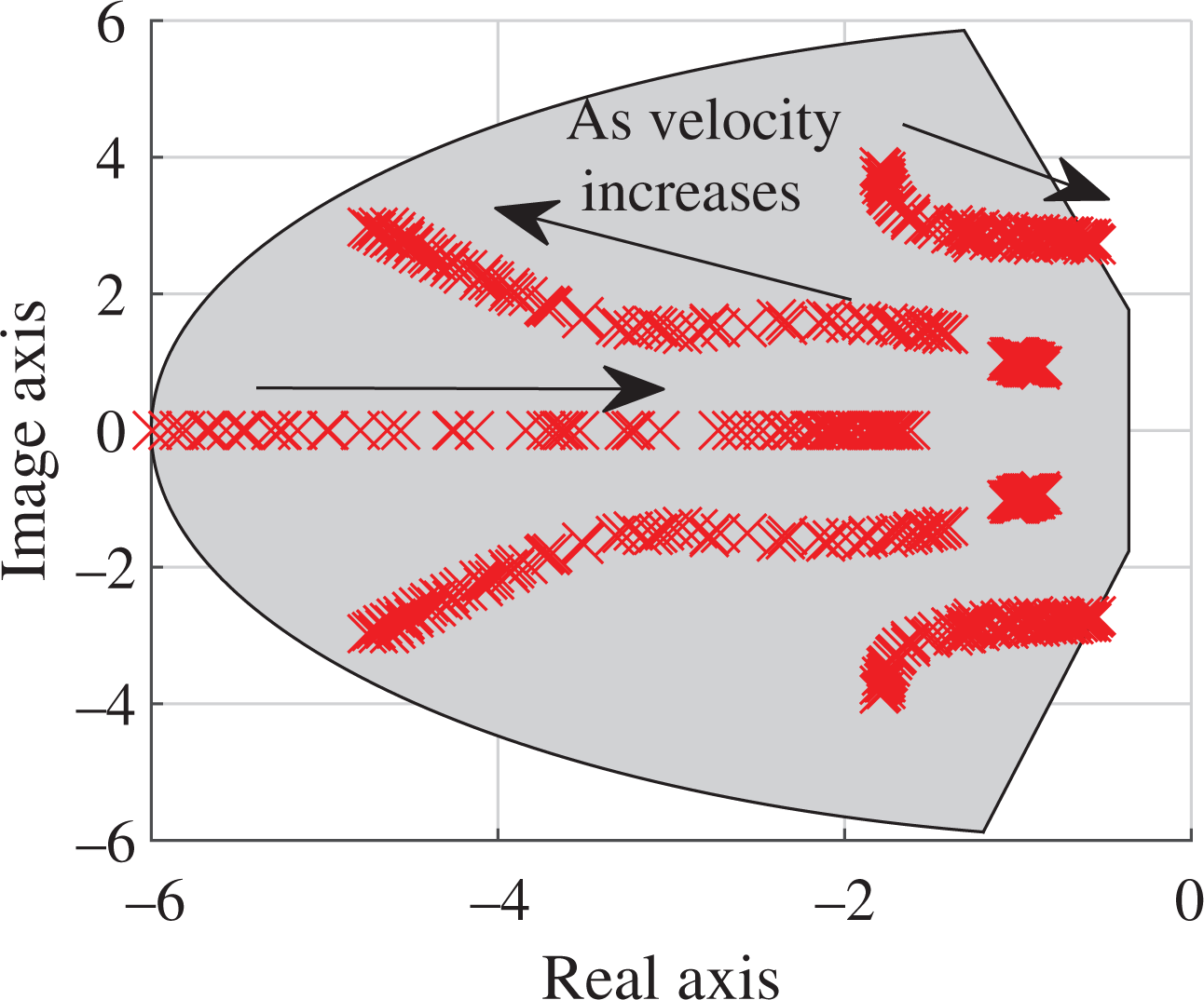
Closed-loop poles as velocity varying.

Figure 10.

Stability boundary of velocity.

Along with the stability of velocity, the range of altitude should be calculated so as to determinate the stability interval of velocity that satisfies the stability requirement of both velocity and altitude. The other vehicle states that α also have been taken into consideration. However, the stability remains as the varying of α from −2° to 6°. Thus, we just consider the altitude stability. The altitude stability interval is set to be Δh = 50 m, which indicate that the acceptable altitude deviation is 50 m.

Once the region satisfied both velocity and altitude, stability is confirmed. The next state feedback controller gain should be determined at the boundary of the region with guardian maps theory so as to guarantee the stability while charging the controller gain. In this study, four stability intervals were found, which cover the entire flight envelope.

Ascent trajectory tracking

With the established gain scheduling algorithm, the tracking simulation of the two types ascent trajectory was performed. The stability interval of altitude with respect to velocity and corresponding control gain vector is examined, which is shown in Figure 11. With the established adaptive controller scheduled by velocity, any flight condition within gray region in Figure 11 will appear to satisfy the required flying quality.

Figure 11.

Altitude stability within the entire flight envelop.

The simulation results of tracking the two types ascent trajectory are shown in Figures 12 and 13, and the control inputs are shown in Figure 14. The ϕ for Scram mode is only limited at the lower speed region, which accords with the theoretical analysis.

Figure 12.

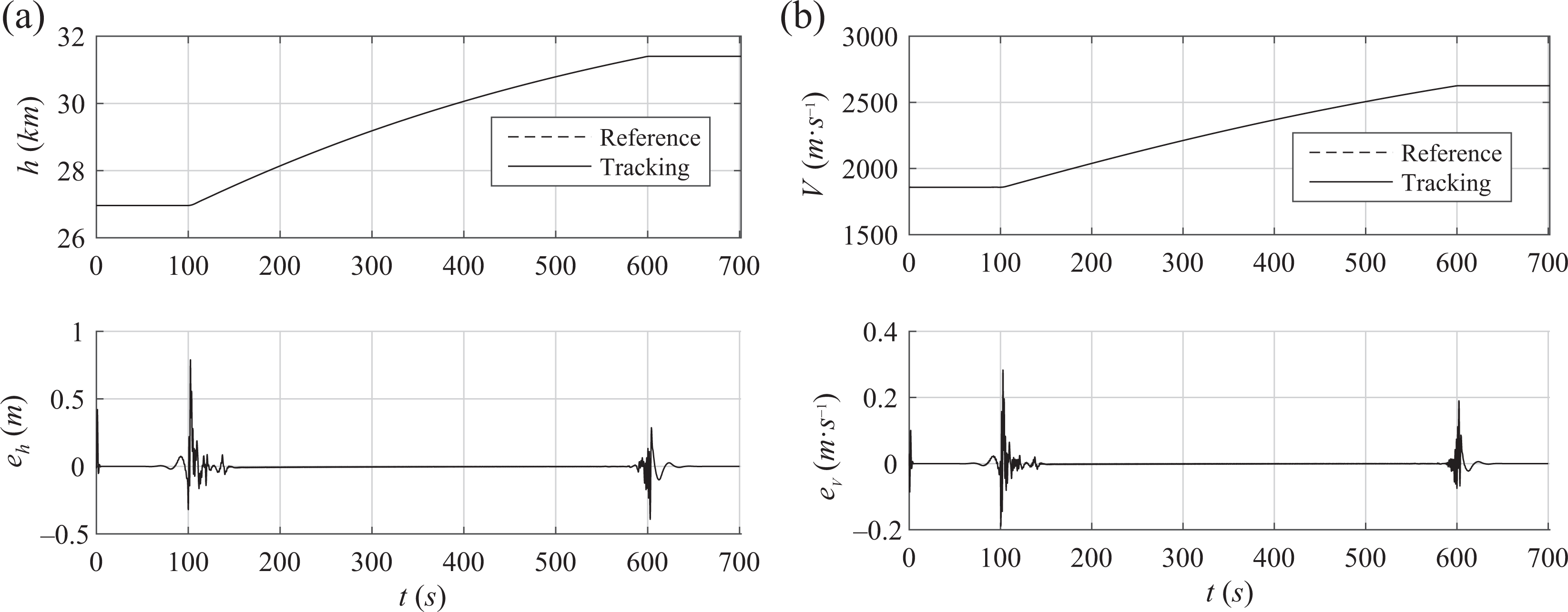
Optimal ascent trajectory tracking without limitation on operating mode. (a) Altitude, (b) velocity.

Figure 13.

Optimal ascent trajectory tracking within Scram mode. (a) Altitude, (b) velocity.

Figure 14.

Control inputs of optimal ascent trajectory. (a) Ram and Scram, (b) Scram.

Conclusions

In this article, a design method of adaptive controller with guardian maps is provided for tracking the climb trajectory. Two general types of ascent trajectories have been taken into consideration: acceleration within Scram mode and acceleration across the Ram–Scram mode transition. The optimal cruise condition is selected as the target point for climb phase, which was optimized for minimum fuel consumption.

A velocity-based LPV modeling and control framework combined with a novel implementation method of nonlinear gain-scheduling controller has been presented. The effectiveness of the controller was demonstrated by simulation results of the responses of the step changes in altitude and velocity.

The simulation of velocity–altitude tracking for a hypersonic vehicle has shown that the closed-loop poles confinement requirements in the target region are satisfied throughout the overall flight envelope with the controller designed by the presented approach. The effectiveness of the gain scheduling algorithm for wide speed range has been verified. The simulation research results will hopefully serve as useful feedback information for improvements for trajectory tracking technique. What’s more, the system represents the excellent tracking performance.