
Abstract
Wireless positioning and tracking technology are key technologies in applying wireless sensor networks and have vital research significance and application value. In this paper, in terms of positioning multiple non-coincident dynamic targets, aiming at the problem of low precision and large computational complexity when locating multiple dynamic targets by the two-step least squares algorithm and the constrained total least squares algorithm, an improved constrained total least squares algorithm is proposed. This algorithm fully considers the constraints, introduces the Lagrangian multiplier technology and the quasi-Newton BFGS iterative formula, avoids the calculation of the Hessian matrix, reduces the amount of calculation, and improves the positioning accuracy. Simulation experiments show that when the measurement error and sensor position error are moderate, the ICTLS positioning algorithm has a smaller RMSE than the TSWLS and CTLS positioning algorithms, showing higher positioning accuracy and stronger robustness. Secondly, aiming at the problem that the target is close to the reference node or any coordinate axis causes the positioning error of the traditional positioning algorithm to increase sharply, an optimized two-step least squares algorithm is proposed. This algorithm corrects the defects of the TSWLS algorithm by selecting the reference station and rotating the coordinate system again, and improves the positioning performance of the algorithm while reducing the amount of calculation.
Introduction
In real life, Wireless Sensor Network (WSN) is widely used and it plays an increasingly important role, and location-based devices are the key core part of all applications, while the positioning target generally occurs in a noisy environment. The measurement error is large, and the error is also large when a single TDOA (Time Difference Of Arrival) ranging technology is used to achieve target positioning. 1 To improve the algorithm’s positioning accuracy, hybrid positioning technology is usually used to estimate the position information of the target. 2 When carrying out position information estimation for multiple moving targets simultaneously, it is usually necessary to use a positioning model combined with TDOA and FDOA (Frequency Difference Of Arrival) to estimate the target speed and position, which effectively improves the positioning accuracy of moving targets. 3 However, when positioning a dynamic target, the position error of the sensor and the measurement error will bring a large positioning deviation. 4 Sun et al. used the TSWLS (Two Step Weighted Least Squares) algorithm to locate multiple moving targets based on the TDOA/FDOA measurement technology combined with the sensor’s position error. The experimental results show that the RMSE (Root Mean Squares Error) of the position estimation can reach CRLB (Cramer-RaoLower Bound) 5 only under the condition of the high signal-to-noise ratio. Since the TSWLS algorithm has poor adaptability to noise errors, the positioning deviation is large, and the positioning accuracy is limited. Chen Shaochang et al. proposed in the literature 6 that the constrained total least squares algorithm considers all coefficient matrices’ noise in the positioning equation and obtains the target’s position coordinates through the Newton iteration method. The experimental results show that this algorithm has better performance than the TSWLS algorithm. However, this algorithm estimates the location information of fixed targets based on TDOA ranging technology and is not suitable for locating moving targets. By analyzing the factors affecting the positioning performance of the TSWLS algorithm, Liu Yang et al. proposed a moving target positioning algorithm based on TDOA/FDOA to correct the positioning error. Without increasing the computational complexity, the positioning error was reduced and the ability to adapt to measurement noise is improved. Yanbin Zou et al. proposed a semi-definite programming (SDP) method, which transforms the common MLE (maximum likelihood estimator) problem into a convex optimization problem, which iterates with the position and velocity obtained by the SDP method as the initial values and updates the velocity using weighted least squares to update the position using SDP, the main advantage of this scheme is that the localization performance is more obvious under medium to high noise conditions, 7 but the position error of the sensor and the sharp decrease in localization performance when the target is close to any axis of the set reference sensor are not considered. In contrast, this paper is mainly based on TSWLS and CTLS, taking into account the sensor position error and measurement error, as well as the localization problem in special scenarios.
Based on the above analysis, this paper mainly studies the positioning of multiple moving targets from two aspects. The first aspect of the research is: Aiming at the positioning of multiple non-coincident dynamic targets, ICTLS (Improved CTLS, ICTLS) positioning is proposed on the basis of the TSWLS and CTLS positioning algorithms. The ICTLS positioning algorithm corrects two defects in the TSWLS algorithm: ① First, the deviation of WLS estimation results increases with the increase of noise error; ② Second, the nonlinear operation introduced in WLS causes large calculation errors, thereby reducing the accuracy of the positioning algorithm. The ICTLS algorithm proposed in the article corrects the connection between the additional variables introduced in the CTLS algorithm and the target position coordinates, and establishes global constraints based on the connection between the target and the additional variables; At the same time, the Lagrangian multiplier technology is introduced to solve the positioning equation. The BFGS iterative formula of the quasi-Newton method avoids the calculation of the Hessian matrix, reduces the amount of calculation and speeds up the convergence speed. Simulation experiments show that when the measurement error and sensor position error are moderate, the ICTLS positioning algorithm has a smaller RMSE than the TSWLS and CTLS positioning algorithms, showing higher positioning accuracy and stronger robustness.
The second aspect of the research is: in view of the fatal flaw in a variety of existing positioning algorithms, that is, when the target approaches a reference sensor or a certain coordinate axis, it will cause a sudden increase in the estimation error of the target position based on the TSWLS algorithm. For this problem, a revised TSWLS positioning algorithm was proposed. The correction algorithm first uses the first step of the TSWLS algorithm to initially estimate the target position, and then re-selects the reference sensor (in principle, the new reference sensor farthest from the target) and the rotation axis according to the estimated target position. Even if the target is approaching the reference sensor or a certain coordinate axis, the correction algorithm also shows superior positioning performance, which makes up for the loopholes in the classic TSWLS series of algorithms.
Algorithm model and positioning principle
Positioning scene
K non-coincident moving targets are randomly distributed in the three-dimensional space, and the true position and speed of the ith target are recorded as
In the formula,
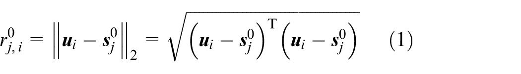
Where

Where
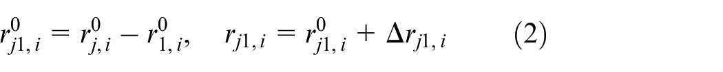
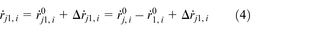
When the target and the sensor move relative to each other, the FDOA measurement value of the target speed information can be obtained from equation (2):
Among them,
For the convenience of the following description, the TDOA and FDOA measurement vectors of the target information are often expressed as a vector equation.8,9 Since the measurement vector of target i can be denoted as
Positioning model
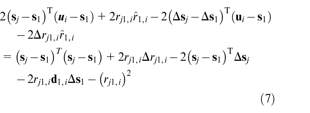
In order to estimate the position and velocity of the target, it is necessary to construct a TDOA/FDOA positioning equation set about the position information of the target and the sensor. To this end, an additional variable
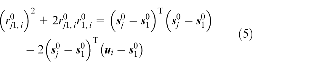
Since the introduced additional variable

Where
Differentiate equation (7) with time to obtain the FDOA equations:
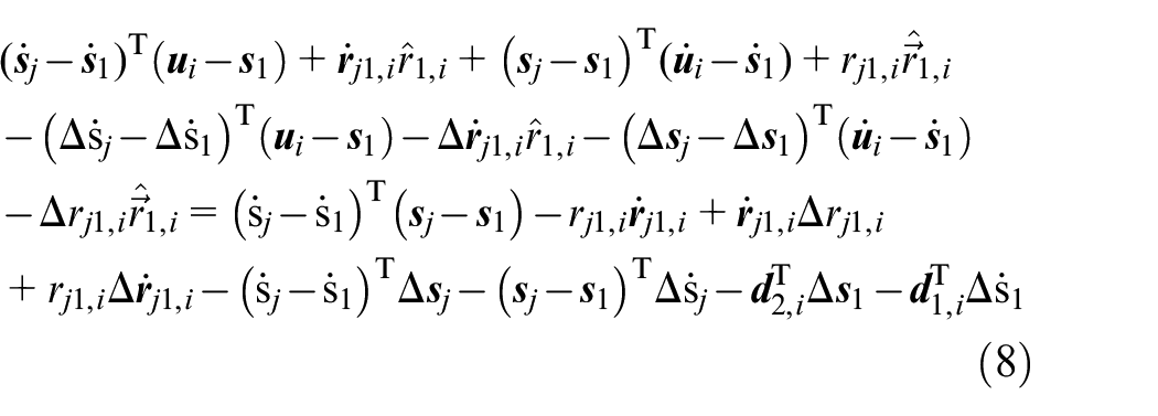
Where,

In the formula,
Optimization
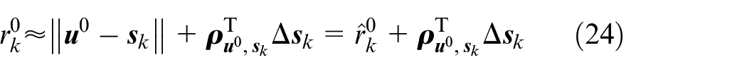
For the above method of solving the target positioning equation, the TSWLS positioning algorithm only considers the error of part of the coefficient matrix in the equation,
12
which causes the target estimated position error to increase; secondly, the TSWLS algorithm considers that the introduced variables

In the formula,
In the formula,

Substituting the deformed formula (12) into the formula (10), the constraint conditions in matrix form are obtained after finishing:

In the formula,
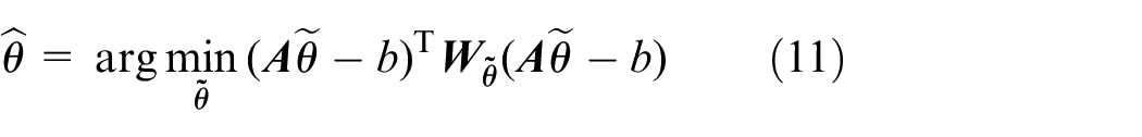
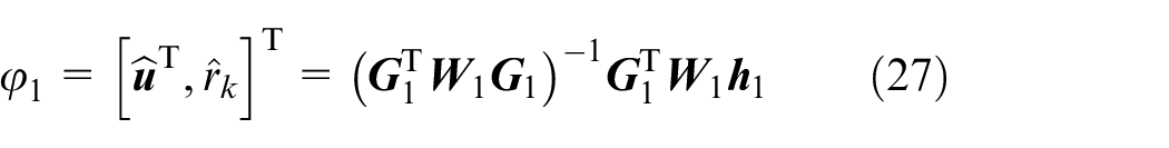
Therefore, the total least squares solution of vector
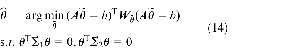
For solving the problem of constrained optimization minimum of formula (14), the Lagrangian multiplier technique is introduced, and the value function of A (10) becomes:
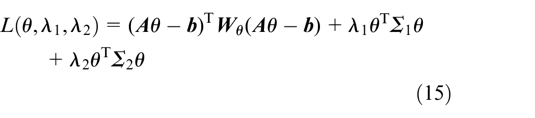
Where
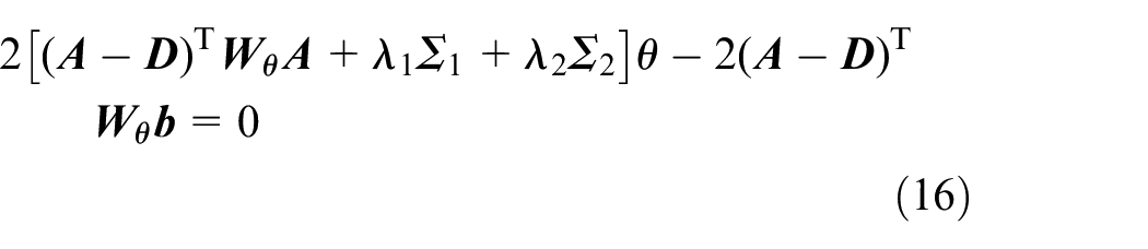
In the formula,
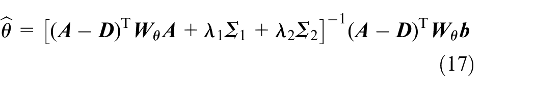
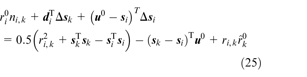
Substituting formula (17) into the constraint formula (13) again, we get:

Equation (18) composes a high-order polynomial equation set about
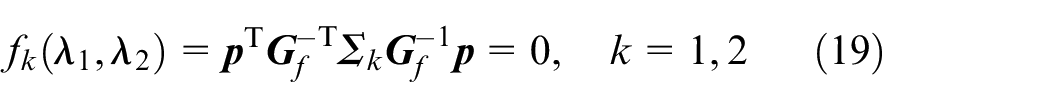
Where,

In the formula,
The specific steps of using the quasi-Newton BFGS formula to iterate are as follows17–20:
Set parameter
Calculate
Calculate the search direction
Let
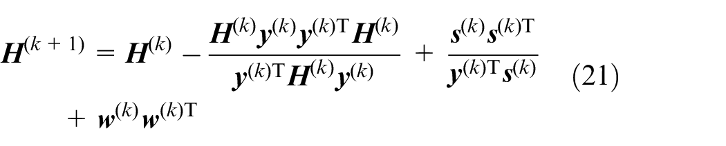
Use the BFGS formula of the quasi-Newton method to update
Finally, the obtained optimal value of
Experimental verification and result analysis
In order to verify the feasibility of the proposed ICTLS algorithm to locate multiple dynamic targets, this section designs three simulation experiments for target location scenarios. In order to compare and analyze the positioning performance of the ICTLS algorithm in detail, the simulation experiment in this article compares the simulation results of the three positioning algorithms TSWLS, CTLS, and ICTLS. The experiment is based on the simulation scheme in Ho et al.
4
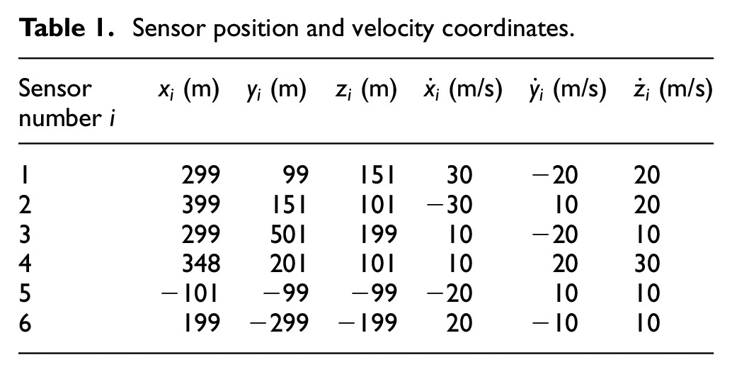
It is assumed that there are six observation sensors in the three-dimensional space. The specific positions and speeds of the sensors are shown in Table 1. In this paper, two targets are taken as examples to carry out the simulation experiment of multi-target positioning, of course, it can also be extended to more targets. The real positions of the two targets to be positioned are
Sensor position and velocity coordinates.
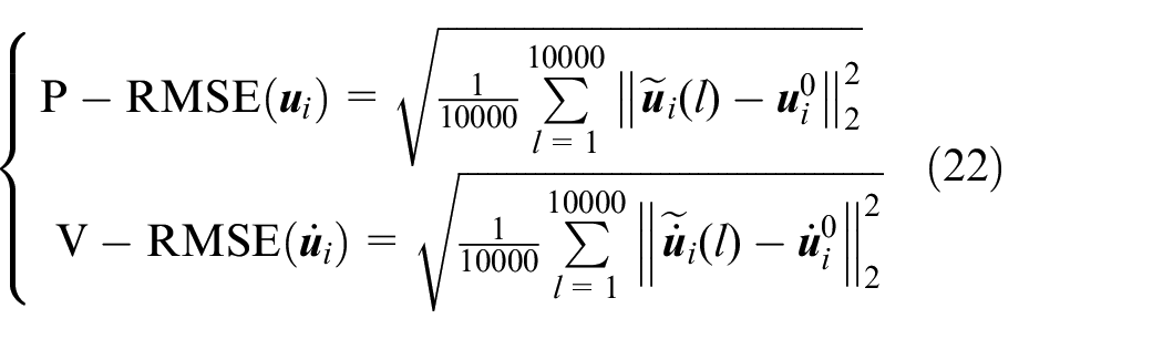
Among them: P-RMSE and V-RMSE respectively represent the RMSE of the estimated position and velocity of the target, and
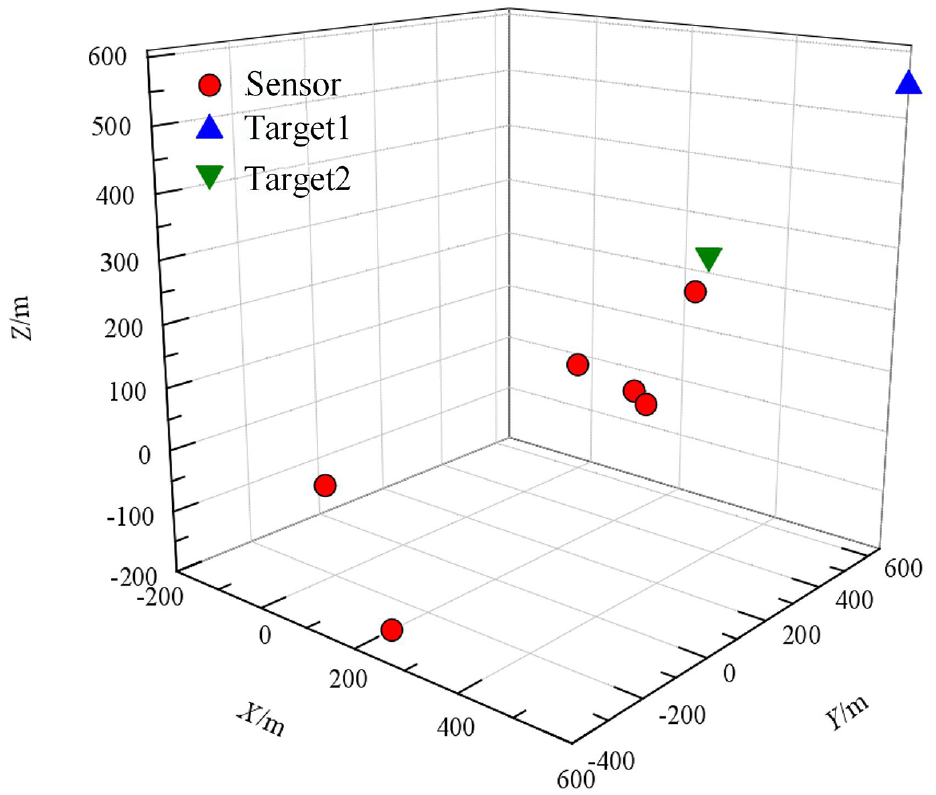
Spatial location distribution of targets and sensors.
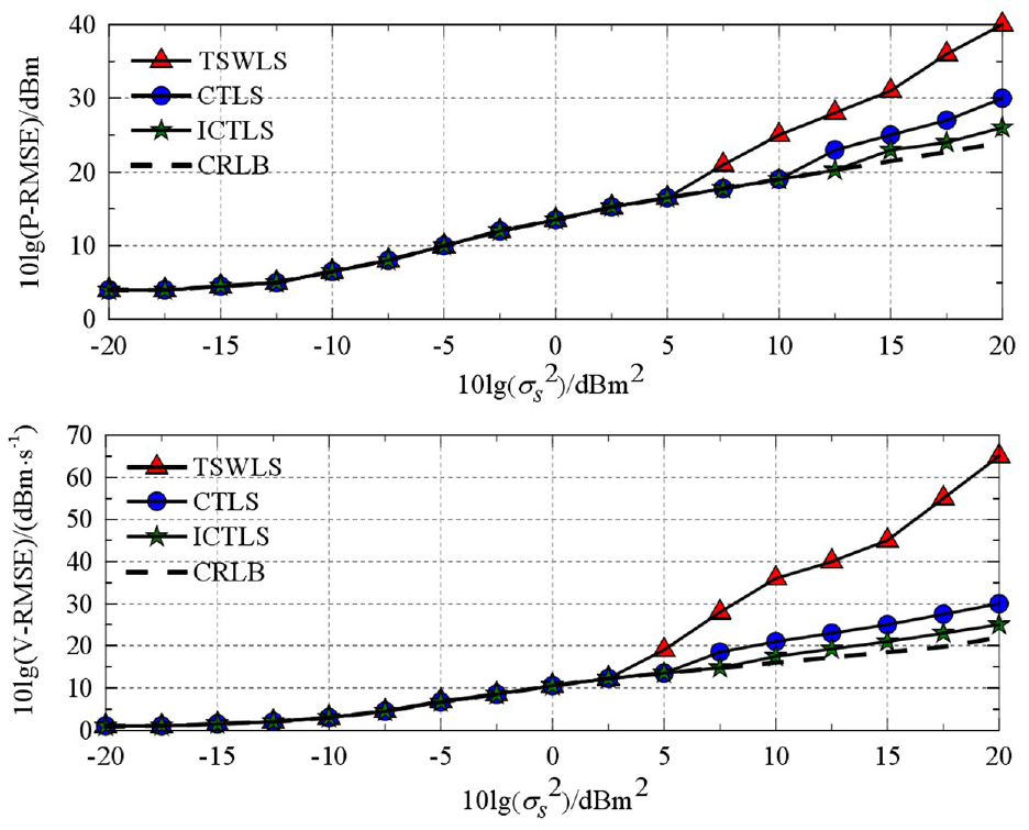
Figure 2 shows the positioning performance of the three positioning algorithms TSWLS, CTLS, and ICTLS when locating a single dynamic target, as well as the comparison results of RMSE and CRLB of the target position velocity estimation deviation. It can be seen from the curve in the figure: For target position estimation, when
Comparison of RMSE and CRLB of the three positioning algorithms under scenario ①.
Therefore, this paper’s ICTLS positioning algorithm has the best performance in positioning dynamic targets among the three positioning algorithms.
In terms of target speed estimation, when
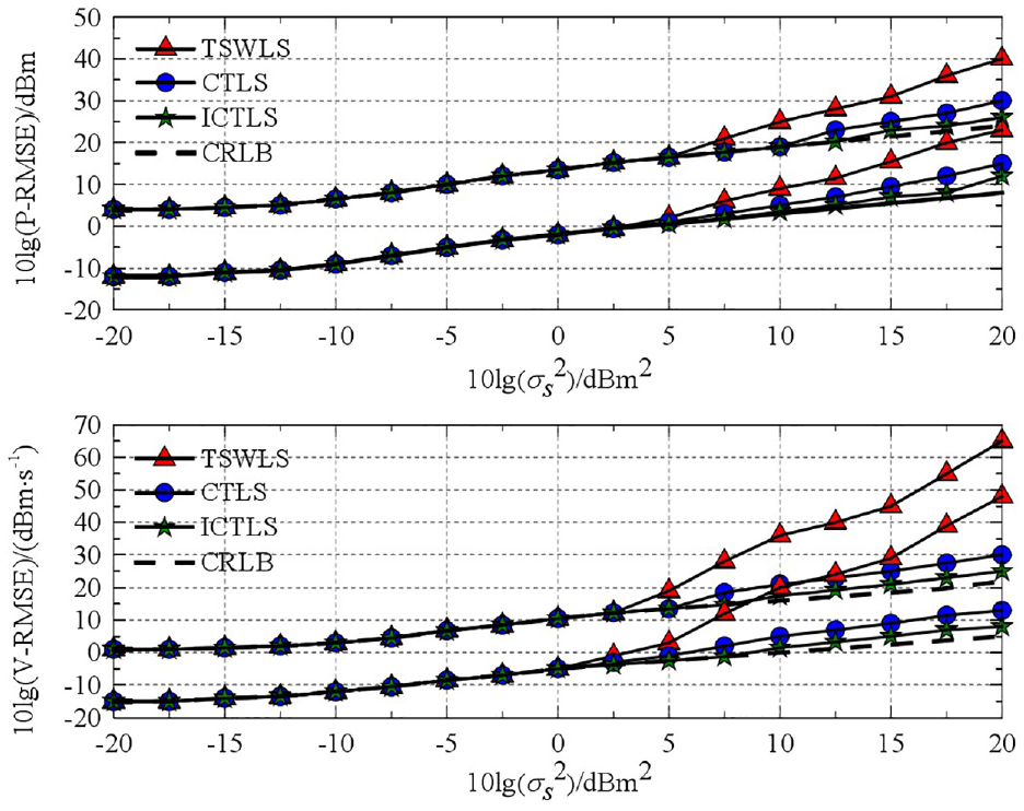
Figure 3 depicts the situation where the RMSE and CRLB of the three positioning algorithms of TSWLS, CTLS, and ICTLS are consistent with the target position and velocity estimation errors when multiple dynamic targets are located. Figure 3 shows the RMSE curve of position and velocity estimation deviation. The upper curve is the RMSE curve of positioning target
Comparison of RMSE and CRLB of three positioning algorithms under scenario ②.
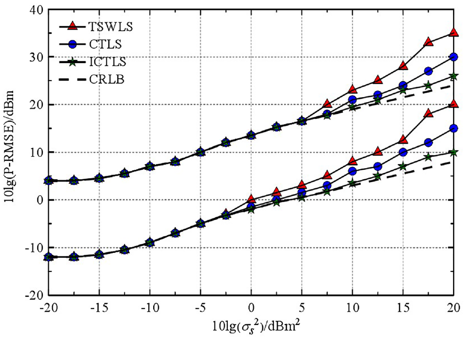
Figure 4 depicts the RMSE and CRLB comparison results of the position estimation errors of the three positioning algorithms TSWLS, CTLS and ICTLS when positioning two static targets. For long-distance target
Comparison of RMSE and CRLB of the three positioning algorithms under scenario ③.
Simulation experiments show that when the measurement error and sensor position error are moderate, the ICTLS positioning algorithm has a smaller RMSE than the TSWLS and CTLS positioning algorithms, showing higher positioning accuracy and stronger robustness. However, when the measurement error and sensor position error are large, the performance of the algorithm in this paper is not as good as expected, which is the limitation of this algorithm.
Math positioning algorithm in specific scenarios
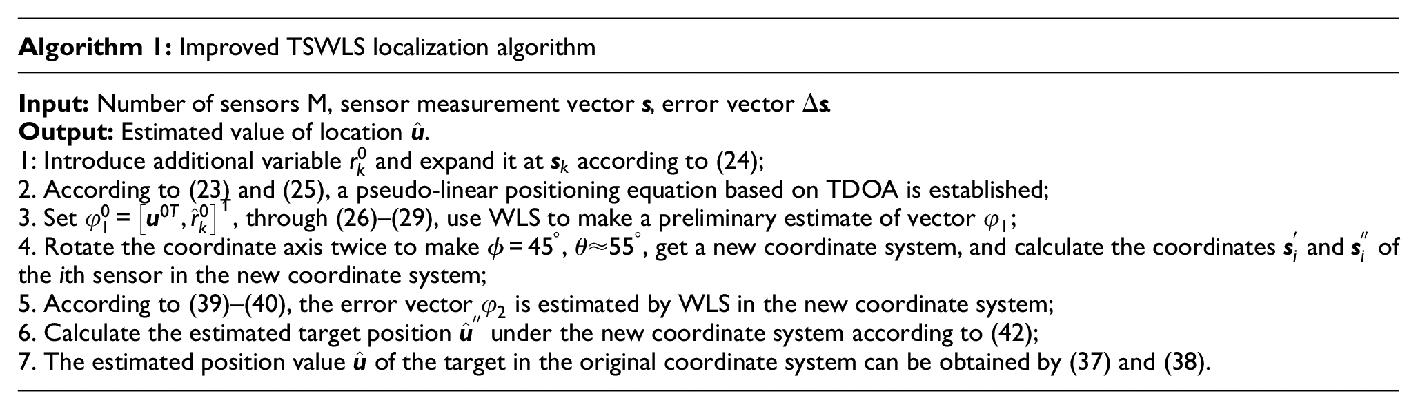
In the previous chapter, based on the estimation of multiple targets’ position by the TSWLS algorithm and the CTLS algorithm, the ICTLS positioning algorithm was proposed. This algorithm fully considered the noise of all coefficient matrices in the positioning equation, introduced the Lagrangian multiplier technology, and used the quasi-Newton The BFGS formula of the method effectively avoids the calculation of the Hessian matrix, reduces the amount of calculation, and comprehensively improves the performance of the positioning algorithm. However, whether it is the classic TSWLS, CTLS positioning algorithm, or the ICTLS positioning algorithm proposed in the article, there is a fatal flaw in locating the target, which leads to a large positioning deviation and a sharp decline in positioning performance. When the target is located at or close to any coordinate axis of the set reference sensor, the above positioning algorithm will have a large positioning deviation, and the positioning performance will drop sharply. In order to avoid the algorithm defects caused by special positioning scenarios, we carefully analyzed the principle of the above algorithm to solve the positioning equation, combined with the measurement error and the position error of the sensor, and introduced a simple and effective strategy based on the TSWLS algorithm, namely, reselecting the reference sensor and the rotating coordinate system avoids the fatal shortcomings of the above positioning algorithm and reduces the target position estimation error in a specific scene. The principle and flow of the improved algorithm to locate the target will be introduced in detail below.
Positioning scene and model establishment
To be better suitable for practical applications, the article considers positioning the target in three-dimensional space. Combining the targets and sensors set in the previous chapter, this section also assumes that M randomly distributed sensors are used to locate a static target
To be more representative, let be the reference sensor and be the origin of the coordinate system. Refer to the positioning scenario and model establishment in Chapter 2, the measurement equation based on TDOA is:

Where
In the formula,
Algorithm optimization
Let

Where,
Therefore, equation (26) becomes a linear equation about
Where
Define
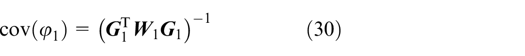
So the covariance matrix of the estimated vector
When the estimated deviation of vector
In the formula,

Where,
Where
In order to further analyze the reason why the re-selectors refer to the sensor, define
In order to facilitate the calculation of the coordinates, the position distribution of the target and the reference sensor is shown in Figure 5. From the geometric relationship in the figure,
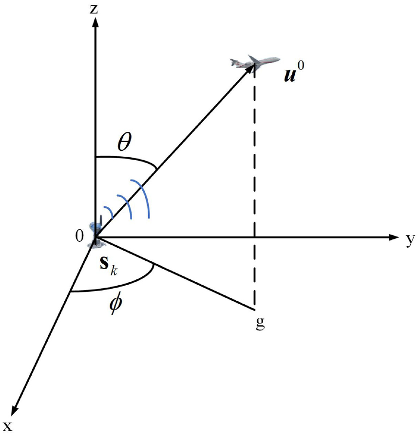
Target and reference sensor distribution.
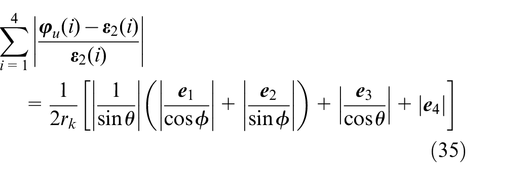
The mathematical expectation of the approximate error formula (35) is:
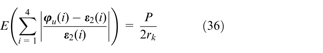
Where
In order to minimize the mathematical expectation formula (36) of the estimated deviation, two steps are required: ① let
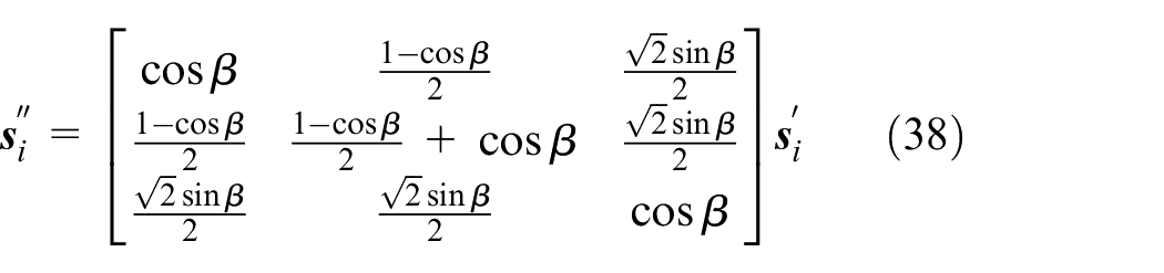
Rotate the coordinate axis for the first time so that
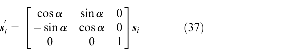
Rotate the coordinate axis for the second time so that
In the same way, the target
The WLS estimation result of the program (32) under the new coordinate system is
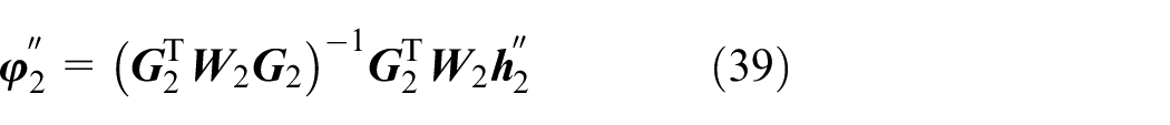
Where
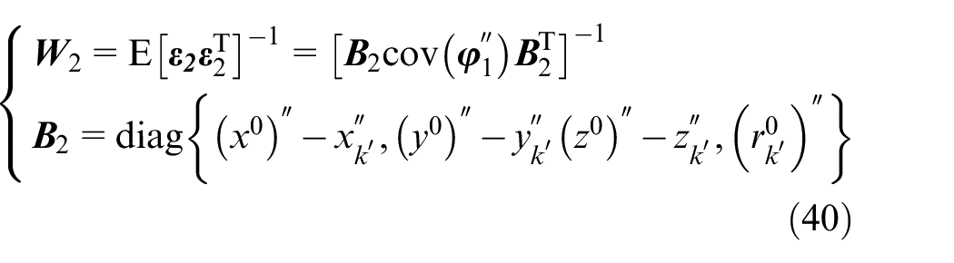
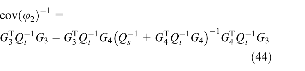
The covariance matrix of the estimated vector
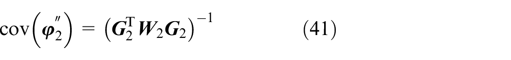
Therefore, the estimated position of the target under the new coordinate system is:
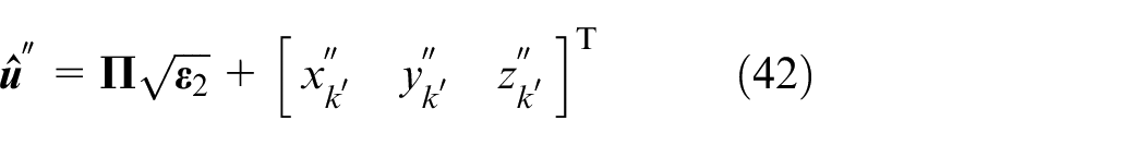
In the formula,
Algorithm performance analysis
In order to facilitate the calculation, we analyze the performance of the optimized algorithm in the paper under the original coordinate system. The following will evaluate the positioning performance of the optimized algorithm by comparing
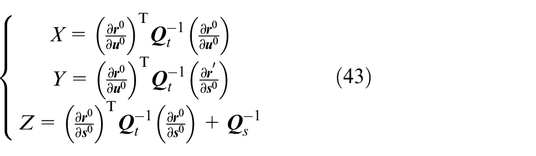
Substituting
In the formula,
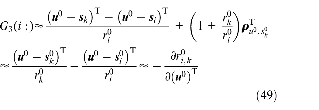
Let the ith row element of
In the same way, if
When the measurement error and the sensor position error are small,
Substituting formula (47) and (48) into formula (46), we get:
Therefore,
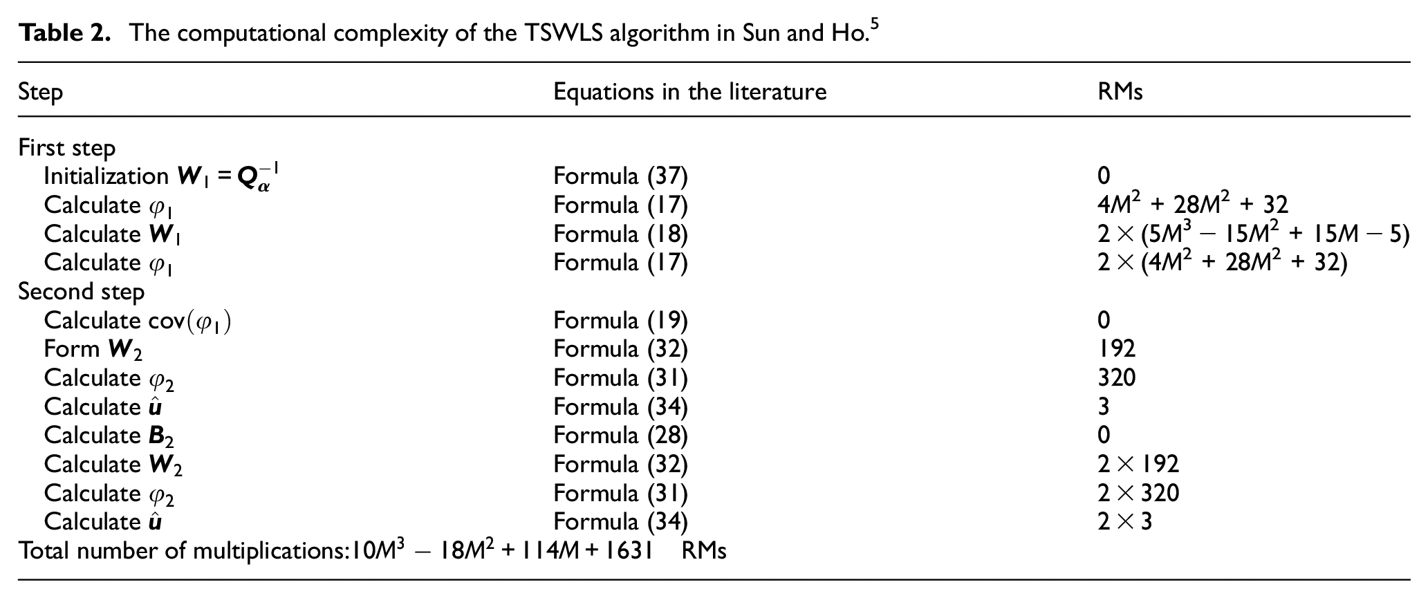
In order to comprehensively evaluate the performance of the optimized algorithm in the paper, we will compare the computational complexity of the optimized algorithm in the paper with the TSWLS algorithm in Sun and Ho. 5 Generally, RM(X) is used to represent the number of multiplications required to calculate the variable X. Usually, N3RMs are required to inverse a N × N matrix, and M × N× PRMs is required to multiply the matrix of M × N and the matrix of N×P. Taking locating a short-range target as an example, the computational complexity of the TSWLS algorithm in Sun and Ho 5 and the optimization algorithm in the paper are shown in Tables 2 and 3, respectively.
The computational complexity of the TSWLS algorithm in Sun and Ho. 5
The computational complexity of the optimized algorithm in this paper.
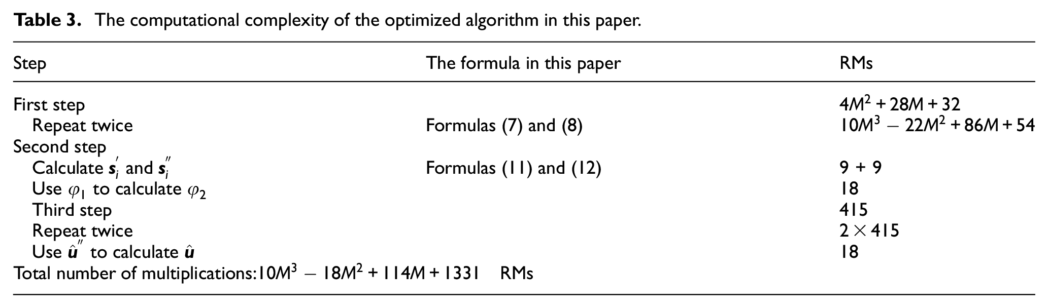
From Tables 2 and 3, it can be seen that the optimization algorithm in the paper requires less total computation than the TSWLS algorithm in literature, 5 and the optimization algorithm in this paper can show better positioning performance, especially when the target is at or close to the reference sensor.
Experimental verification and result analysis
This section compares the proposed optimization algorithm’s performance and the TSWLS algorithm for positioning targets through simulation experiments in two positioning scenarios. The two positioning scenes are ① special positioning scene, that is, the target is located at or close to the reference sensor; ② random positioning scene, that is, the target and sensors are randomly distributed in three-dimensional space. The experiments in the two positioning scenarios were run 5000 Monte Carlo experiments on a PC, and the positioning performance of the algorithm was analyzed by comparing the MSE and deviation of the position estimation of the two algorithms. The MSE and bias of the position estimate are defined as 26 :
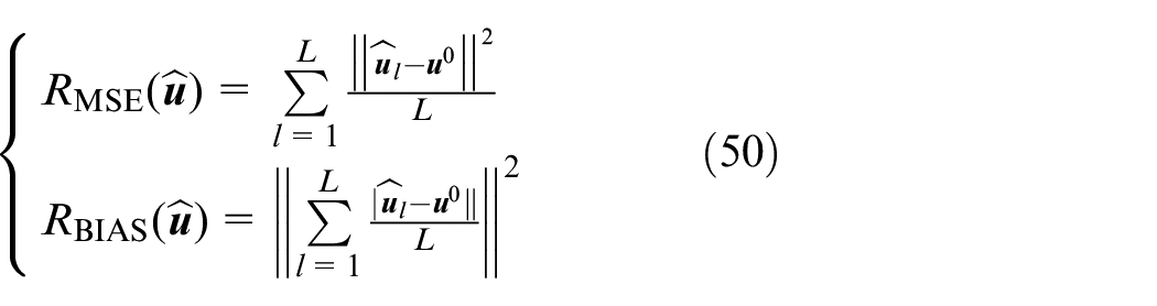
Where
Target positioning in a specific scene
There are two targets to be located in the monitoring area, one is the short-range target
Real position coordinates of the sensor.
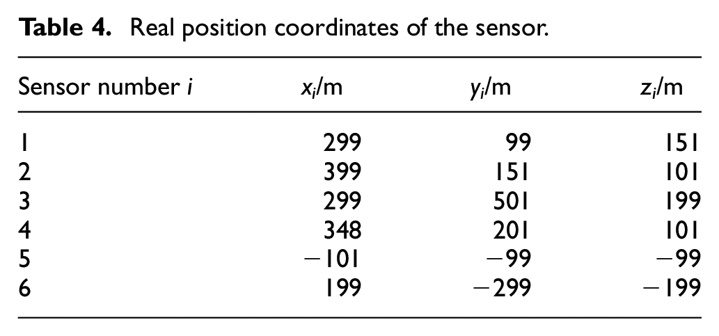
The distribution of targets and sensors in space is shown in Figure 6, assuming that A is the reference sensor. We compare the position estimation deviation and MSE to evaluate the positioning performance of the TSWLS algorithm in Sun and Ho 5 and the optimized algorithm in the paper.
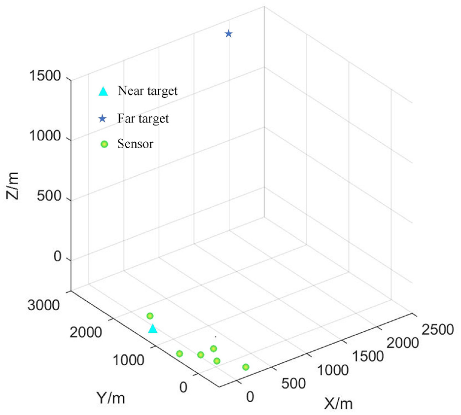
Target and sensor position distribution in a specific scenario.
Figure 7 depicts the relationship between the MSE and the deviation of the short-distance target position estimated by the two algorithms and the sensor position error variance. As can be seen from the figure,
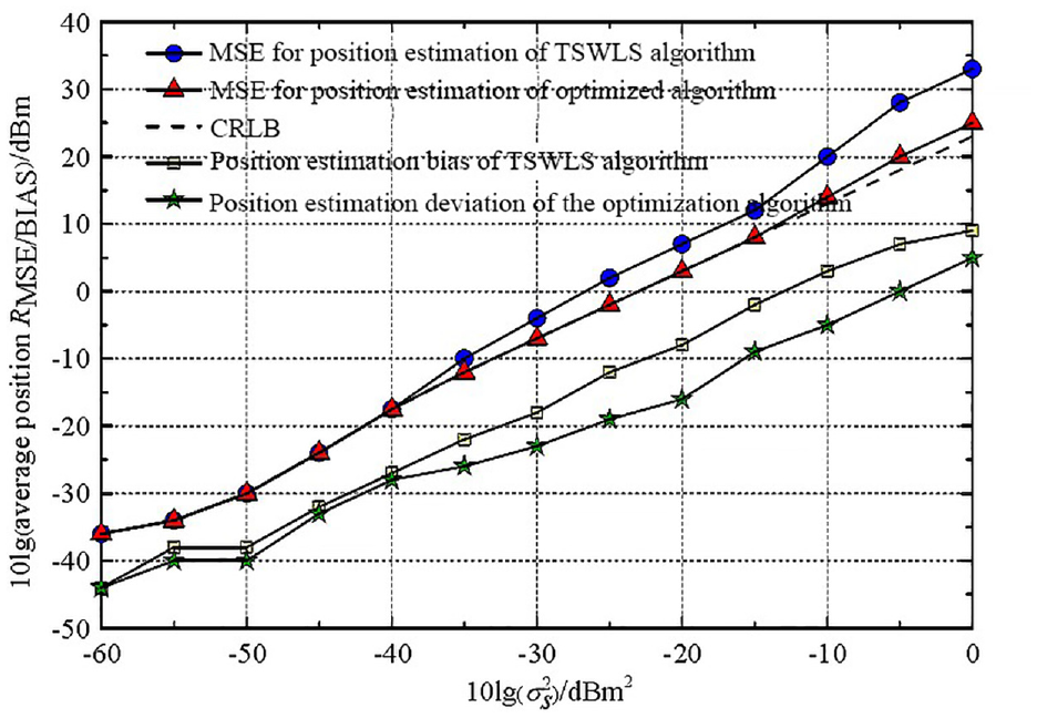
Performance comparison of two algorithms when locating close-range targets.
Figure 8 shows the relationship between the MSE and the deviation of the long-distance target position estimated by the two algorithms and the sensor position error variance. It can be seen from the curve in the figure that when
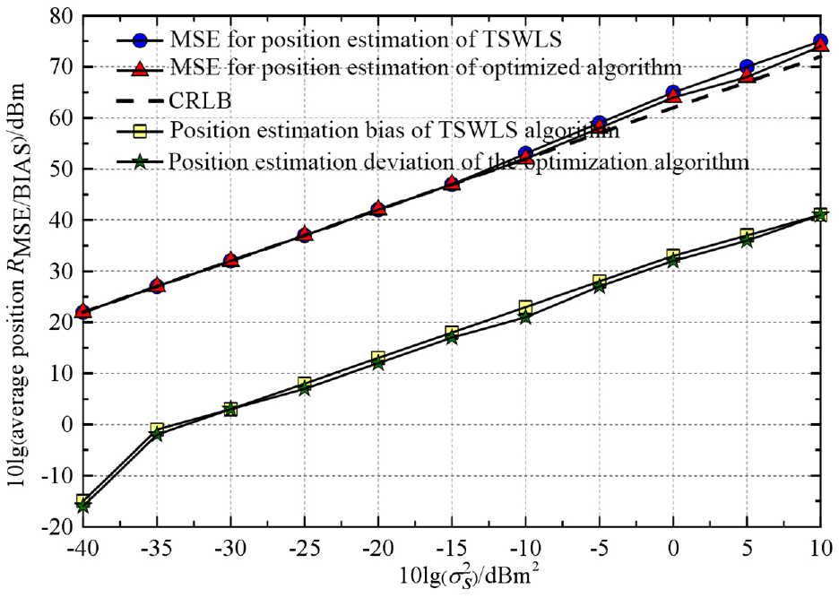
Performance comparison of two algorithms when locating long-distance targets.
Figure axis labels target positioning in random acenes
Hundred target sources are randomly distributed in the setting space, and the target sources are randomly distributed in a cube with a side length of 600 m. Similarly, 100 sensors are randomly distributed in a cube with a side length of 200 m, and the centers of the two cubes coincide. Randomly select six sensors and one target as a positioning scene, and run 5000 Monte Carlo experiments on the PC to locate each scene’s target. The settings of other parameters are the same as those of target positioning in a specific scene. The spatial distribution of targets and sensors is shown in Figure 9.
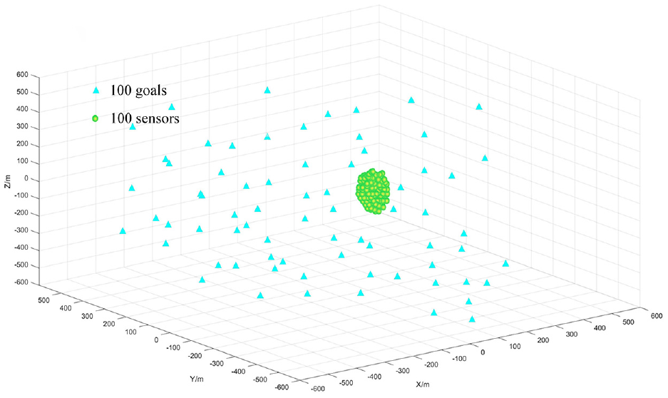
Target and sensor location distribution in random scenarios.
Figure 10 depicts the relationship between the MSE and deviation of the target position estimated by the two algorithms and the variance of the sensor position error when the target and sensors are randomly distributed. It can be seen from the graph curve that when
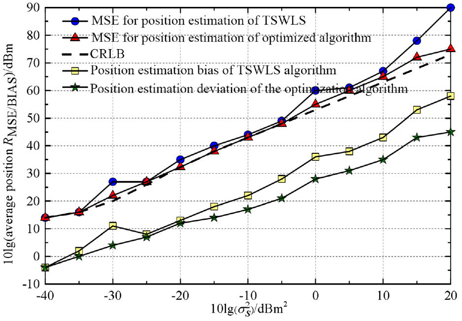
Performance comparison of the two algorithms when targets and sensors are randomly distributed.
Figure 11 shows the relationship between the average MSE and the deviation of the target position estimated by the two positioning algorithms with the number of sensors. In the experiment, the number of sensors is gradually increased from 3 to 8. Simultaneously, set the average position error variance of the sensor to
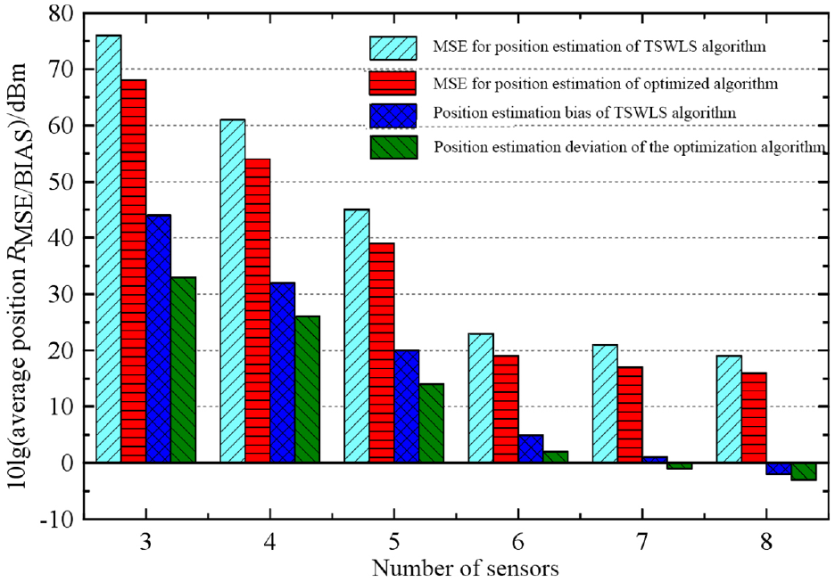
The relationship between position estimation MSE and deviation and the number of sensors.
In the presence of both sensor position error and measurement error, this section carefully analyzes the solution process of the TSWLS algorithm and corrects the fatal defects in TSWLS by re-selecting the reference sensor and rotating the coordinate system, thus optimizing the TSWLS algorithm and improving the positioning performance of the TSWLS algorithm in general. However, the introduction of new operation steps in the optimization algorithm leads to a slight increase in the amount of operations and a slight increase in the time used to locate the target, which is a reflection of the limitations of the algorithm in this paper, and it is evident that any high-precision localization algorithm comes at the expense of the amount of operations.
Conclusion
Aiming at the positioning problem of multiple non-coincident targets, the ICTLS positioning algorithm is proposed. By analyzing the shortcomings of the TSWLS algorithm when positioning multiple targets, the proposed ICTLS algorithm establishes global constraints based on the relationship between the target and additional variables, and introduces Lagrangian multiplier technology to solve the positioning equation using the quasi-Newtonian BFGS iterative formula. Avoiding the operation of the Hessian matrix and reducing the calculation amount of the algorithm. The proposed ICTLS algorithm shows better positioning performance and strong robustness.
The optimized positioning algorithm of TSWLS solves the hidden dangers in many positioning algorithms; when the target is located at or close to the reference sensor, the estimation error increases suddenly. Based on retaining the closed-form solution, the optimization, the algorithm effectively reduces the position estimation error by reselecting the reference sensor and the rotating coordinate system, corrects the TSWLS algorithm’s defects, and comprehensively improves the positioning performance of the TSWLS algorithm.
Footnotes
Declaration of conflicting interests
The author(s) declared no potential conflicts of interest with respect to the research, authorship, and/or publication of this article.
Funding
The author(s) disclosed receipt of the following financial support for the research, authorship, and/or publication of this article: This work was supported in part by the National Natural Science Foundation of China under Grant 61640308, Grant 61773395, and in part by the Natural Science Foundation of Hubei Province of China under Grant 2019CFB362.