Sage Journals: Discover world-class research

Abstract

Rotor dynamic balancing is essential in rotor industrial. The conventional balancing methods, including the influence coefficients method and modal balancing method, are effective, but lack economy and sufficient usage of the data. To overcome the disadvantages of the conventional balancing methods, a balancing method using unsupervised deep learning without weight trails had been proposed. The proposed network could identify the unbalanced forces from the data observed from just one run of the rotor and without labels. To validate the novel balancing method, an experimental rig is well-designed and established. Experimental validation and comparison with influence coefficients method are conducted. The experimental results show that the proposed balancing method gives consideration to both cost and accuracy. Compared with influence coefficients method, no extra weight trail process is needed and balancing performances are comparative. The experimental rig can be used for proving the scheme and for further same kind of research.

Keywords

Rotor balancing unsupervised deep learning weight trial experimental rig balancing experiment

Introduction

Rotor Balancing is a type of analysis that compares the vibration profile with the rotation of a mechanical element to characterize inconsistent weight distribution around the diameter while calculating the amount and position of the weight necessary to offset the net imbalance. As rotor imbalance may lead to malfunction, such as rotor rub-impact and bearing wear, and even to catastrophic failure,¹ the rotor balancing is a traditional technology, but still important in nowadays rotor industry. Any mass that is not rotating around its center of mass will produce vibration. Asymmetry of the structure along the rotating axis and small changes in density and thickness of the material cause imbalances. And imbalance distribution leads to additional force and moment onto the rotor. Every single rotor need several times of balancing including factory balancing² and on-site balancing³ before implementation and online balancing⁴ while in working condition.

For decades, dynamic balancing methods are developed based on two mature ideas. One is the modal balancing method (MBM) and the other is the influence coefficients method (ICM). Bishop and Gladwell⁵ proposed the MBM at first and it was optimized afterward.⁶ The ICM was proposed by Goodman⁷ firstly and perfected by Lund and Tonnesen.⁸ The central theory of the MBM is to balance the first $N$ modal unbalanced responses by adding trail weights to $N$ balance surfaces and the speed of the system should be close to the critical speed of each mode. While for the ICM, the main technique is to identify the unbalanced parameters by the linear relationship between the trail weights and vibration responses of the rotor system. However, the disadvantages of the conventional balancing method are obvious. ICM and ICM-like methods^9–13 are easy to operate. But, more measuring data of the responses at different measuring points with different rotating speeds are usually necessary to achieve better performance. As for the ICM or like approaches, the inappropriate position of measurement points may result in an ill-conditioned coefficient matrix and lead to the failure of this method. Meanwhile, due to the limitation of the working conditions of the rotor system, high speed measures for a long time may lead to decreasing in the system sensitivity at high modes. Several times of weight trial processes are essential. Thus, the cost of the balancing process keeps high. MBM and MBM-like methods^14–18 use prior knowledge of the system to identify imbalance. However, the change of the stiffness and damping, that is the support properties of bearings and high damping systems would affect the identification results of rotor imbalances when balancing by the MBM. If we have enough prior knowledge about the rotor, the weight trail times can be reduced significantly by introducing the full set of modals.

Cost and accuracy are two main considering points in the rotor balancing process. Therefore, some dynamic balancing methods based on advanced technologies are proposed by researchers and good performances in some specific cases were observed. Rotor balancing methods have been developed from various perspectives including algorithm modification and the introduction of advanced technology. For example, Zhao et al.¹⁹ proposed a transient characteristic-based balancing method (TCBM) combined with dynamic load identification (DLI) technique to identify the unbalance parameters of the general rotor system. Li et al.²⁰ proposed a novel modal balancing technique without trial weights by combining the modal balancing method with the finite element method. Zhang et al.^21,22 identified an unbalance response of a dual-rotor system with a slight rotating speed difference by whole-beat correlation method and non-whole beat correlation method respectively. Yue et al.²³ presented an innovative modal balancing process for estimating the residual unbalance from different equilibrium planes of the complex flexible rotor system. Yu et al.²⁴ proposed a new adaptive proportional-integral control strategy for rotor active balancing systems during acceleration. Li et al.²⁵ proposed a novel disturbance-observer-based field dynamic balancing strategy for active magnetic bearings (AMB) equipped machinery. Zheng and Wang²⁶ presented a novel high-precision field balancing method based on regular control mode without trial weight. Ait Ben Ahmed et al.²⁷ presented and validated a hybrid method through a series of experiments for balancing of rigid and flexible rotors at a constant rotational speed. However, these methods did not involve the history data into the balancing process.

Deep learning technologies are usually used to address the input identification problem by learning the inverse mapping from data. To rotor balancing problem, the learning of the mapping can be processed by the same data used for the balancing process. That means no extra data or prior knowledge are needed for rotor balancing. Based on the truth, the author proposed a novel balancing method²⁸ with deep learning technology. To validate the deep learning based method and compare it with the conventional balancing method, a testing rig is carefully designed and established in this work. Thus, the deep learning based method can be validated and investigated in a practical way. And the experimental evidence of the novel balancing method makes the conclusion more convinced.

In the following, the methodology will be introduced in Section 2. In Section 3, the detailed set up process of the experimental rig is described. In Section 4, the application of the proposed balancing method on the rig will be conducted. More detailed testing results and comparisons will be performed. Finally, the paper is concluded in Section 5.

Methodology

Describing the equations of motion for mechanical systems has been extensively studied and various formalisms to derive these equations exist. The most prominent are Newtonian-, Hamiltonian-, and Lagrangian-Mechanics.²⁹ Within this work, based on Newtonian-Mechanics, a mapping model $f$ can be used either to predict the change of system state in a forward way or identify the input $τ$ in its inverse form $f^{- 1}$ , that is,

f (q, \dot{q}, τ) = \overset{\cdot\cdot}{q}, f^{- 1} (q, \dot{q}, \overset{\cdot\cdot}{q}) = τ,

(1)

where $q$ refers to the generalized coordinate vector, and $\overset{\cdot}{q}$ and $\overset{\cdot\cdot}{q}$ are corresponding generalized velocity and acceleration vectors. Approximating $f$ and $f^{- 1}$ with deep networks, that is,

\hat{f} = \hat{f} (q, \dot{q}, τ; α), {\hat{f}}^{- 1} = {\hat{f}}^{- 1} (q, \dot{q}, \overset{\cdot\cdot}{q;} β),

(2)

the forward mapping model and inverse mapping model could be learned from data, where $\hat{.}$ means an approximation and $α$ and $β$ are network parameter tensors.

Learning the model from data has been addressed in the references by either system identification or supervised black-box function approximation. For instance, Ting et al.³⁰ developed a Bayesian parameter identification method that can automatically detect noise in both input and output data for the regression algorithm that performs system identification. Haruno et al.³¹ proposed a modular architecture, the modular selection and identification for control model, for motor learning and control based on multiple pairs of forward (predictor) and inverse (controller) models. Calinon et al.³² presented and evaluated an approach based on Hidden Markov Model, Gaussian Mixture Regression, and dynamical systems to allow robots to acquire new skills by imitation. Ledezma and Haddadin³³ introduced a conceptual framework for the construction and training of first-order principles networks and described the proposed estimation method in detail. All these works modeled the forward and afterward mappings with specific neural networks.

In detail, for a mechanical system identification problem, the inverse model learns the mapping function from joint configuration $(q, \overset{\cdot}{q}, \overset{\cdot\cdot}{q})$ to input force $τ$ . Using the samples $(q, \overset{\cdot}{q}, \overset{\cdot\cdot}{q}, τ)$ observed from the real mechanical system, the parameters of the deep neural network can be learned by minimizing the error between the real value of the sample and the predicted value. Starting from equation (1), supervised learning approaches would train the parameters by minimizing a function (e.g. $ℓ_{2}$ norm) of error between the prediction of equation (1) and measured input force $τ$ , that is, by solving an optimization problem described as

β^{*} = \underset{β}{\arg min} ℓ_{2} ({\hat{f}}^{- 1} (q, \overset{\cdot}{q}, \overset{\cdot\cdot}{q}; β), τ)

(3)

In the case of applying these theories to the rotor balancing problem, the training dataset used for training the proposed network can be get from state variables and their derivatives in different time intervals or at different time points. Enough training data can be get by just one run of the rotor system. Multi-weight trail processes are not essential then.

However, the unbalanced force can’t be measured directly. Luckily, the bearing force can be gotten indirectly through the bearing support by

τ_{sm} = ma - F

(4)

where $m$ is the mass matrix of the bearing support, $a$ is the acceleration vector of the bearing support and $F$ is the force vectors measured by dynamic force sensors.

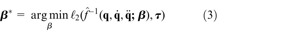
Because the labeled unbalanced force can not been got, only the bearing forces estimated by equation (4) are involved. Then the optimization function should be adjusted to

β^{*} = \underset{β}{\arg min} L (({\hat{f}}^{- 1} (q, \overset{\cdot}{q}, \overset{\cdot\cdot}{q}; β))_{s}, τ_{sm})

(5)

where $L$ can be an arbitrary loss function.

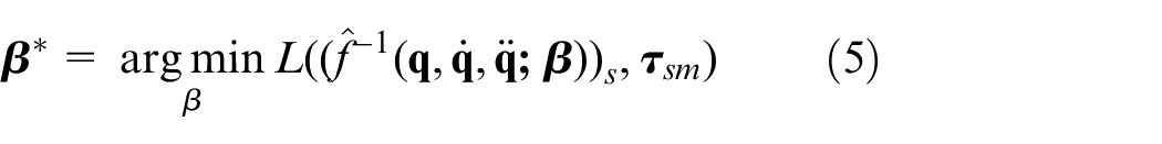
To apply equation (3), a method to learn the mapping from system states to bearing forces directly, while the unbalanced forces to be learned unsupervised has been proposed.²⁸ The overview of the method and the architecture of the unsupervised network are shown in Figure 1. As Figure 1(a) illustrated, there are three steps for the whole balancing method. In the first step, the data get from the system should be pre-processed, that is, the displacements should be derived to get the velocities and accelerations and bearing forces are obtained from the measured support forces by equation (4). Because, in the rotor system, vibration displacements of the disk and shaft can be easily measured by eddy current sensors, while the velocity and acceleration can not. A pre-processing module should be introduced to derive the measured displacement. Secondly, the proposed network is set up. The architecture and the un-trainable parameters should be determined. Based on the loss function chosen, the training process is done by backpropagation. The trainable variables are updated until the standard of the optimization is met. Thirdly, the predicted unbalanced force should be fit to get the amplitude and phase of the harmonic type of force. Based on the identification results, the weight adding and weight reducing processes should be conducted on the rotor. An additional test to verify the performance of the balancing is necessary obviously.

Figure 1.

Flow chart of the balancing method²⁸– (a) with the unsupervised deep learning network – (b), where Conv3–128 means convolutional layer with 128 filters of size 1 × 3.

In the detail of Figure 1(b), the neural network module can be an arbitrary type, only changing the 2-dimensional input data into 1-dimensional output data. After the neural network module, three 1-dimensional convolutional layers are applied. The first one has 128 filters with the size of 1 by 3. The convolutional calculation is applied to the output from the network module. After the feature extraction process, the low order representations of the data are obtained. The “Relu” activation function is applied so that the low order representations are activated. The second convolutional layer has 64 filters with the size of 1 by 3. Then the high order representations are extracted and activated. The third convolutional layer has just one filter with the size determined by the dimension of the expected input force, that is the concatenation of the dimension of the indirectly measured bearing force vector $τ_{sm}$ and the dimension of the unknown unbalanced force vector $τ_{s}$ . Thus the final output can be expected as input data, in which $τ_{s}$ is used to solve the optimization problem described by equation (5), the $τ_{u}$ is used as the prediction of the unbalanced force. It is noted that the parameter sharing mechanism of convolutional networks ensures that all the trainable variables in the proposed network would be updated during backpropagation process.

Set up of experimental rig

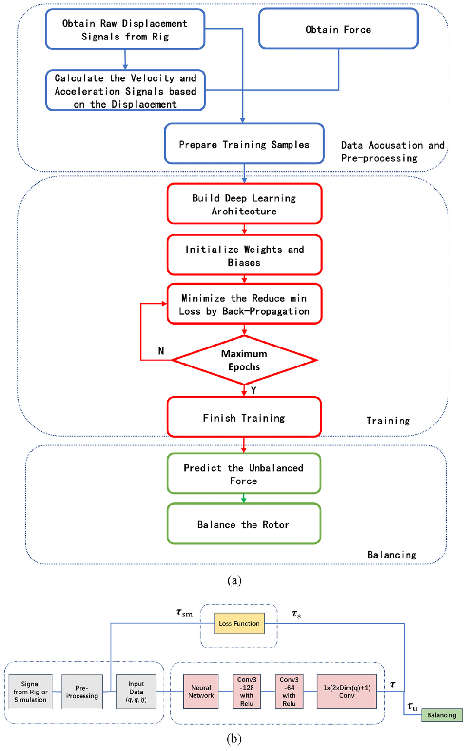
To study the rotor balancing problem in a practical way, an experimental rig is established. The overview of the rig is shown in Figure 2. The rotor rig is composed of a rotor base, a speed-regulating motor, two bearing supports, an elastic coupling, a rotor shaft, four rotor disks, six eddy current sensors, two dynamic force sensors, a photoelectric test sensor and a signal amplification and storage module. The fundamental part of the rig is a single rotor with four disks and two ball-bearing supports. The rotor is driven by a speed-regulating motor with the maximum power of 148 W. The motor driver rectifies the 220 V AC power supply and outputs a PWM signal to drive the rotor. Connecting with an elastic coupling, the rotor rotating speed can be adjusted from 0 to 2000 rpm. The rotor is supported by two ball bearings, which are mounted elastically on the base. The distance between two bearings is 375 mm. Between them, four disks are installed equidistantly. Each disk has a diameter of 50 mm and a thickness of 16 mm. The rotor shaft has a length of 560 mm and a diameter of 10 mm. From right to left in the front view of the rig (Figure 2(b)), two bearings and four disks are numbered from #1 to #6 successively.

Figure 2.

Overview of the experimental rig from (a) top direction, (b) front direction, and (c) side direction.

Six eddy current sensors are installed near each numbered nodes separately through brackets to collect displacement signals of the horizontal vibration of the chosen nodes. Two dynamic force sensors are amounted at #1 node and #6 node to measure the forces, which will be used to estimate the horizontal components of bearing forces. A photoelectric sensor is installed on the side of the coupling through a bracket and a piece of reflective paper is attached to the coupling. The photoelectric sensor generates a pulse with the rotating frequency. This pulse signal serves as a reference for the rotating speed and initial vibration phase. A signal collection equipment with type of DH5922N is used to amplify, rectify and store the measured signals. The sampling frequency can be adjusted from 10 to 10,000 Hz. The sensors used to measure the data are shown in Figure 3.

Figure 3.

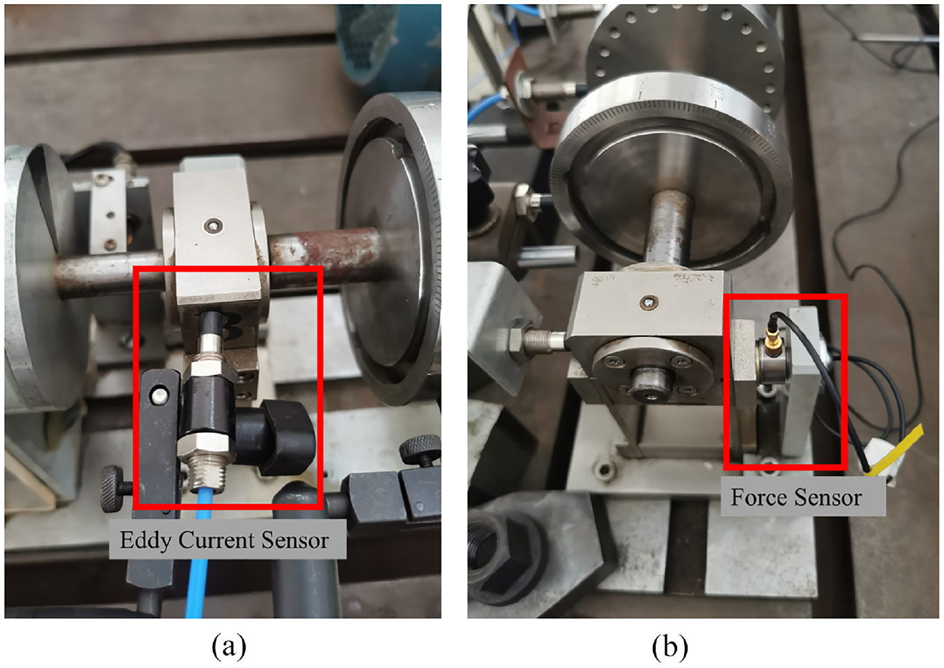
Instruction of the sensors implemented in the experimental rig: (a) Eddy current sensor and (b) dynamic force sensor.

Experimental results analysis

Experimental results before balancing

Based on the rig set up in Section 3, the mechanical model of the rig can be expected to ordinary differential equations. Thus, the responses of the rotor should be a type of harmonic ones with different frequencies. And the component with a frequency corresponding to the rotating speed is the one excited by unbalanced forces. The responses are measured by the eddy current sensors at numbered nodes. The raw responses from the rig described by Figure 2 are shown in Figure 4. From Figure 4, harmonic types of responses are seen. Due to the high stiffness of the bearing, the amplitudes of the responses at bearing nodes (Figure 4(a) and (f)) are obviously smaller than those at disk nodes (Figure 4(b)–(e)). And because of some other disturbances with different frequencies, for instance, constant components from the deviations of the sensors and double frequency component induced by the coupling, the responses contain many components with different frequencies.

Figure 4.

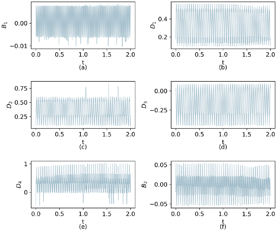
Raw responses measured by eddy current sensors at (a) #1 node, (b) #2 node, (c) #3 node, (d) #4 node, (e) #5 node, and (f) #6 node.

The frequency of vibration caused by imbalance distribution equals the rotating speed. Thus, the raw measured responses need pre-processing before using for the balancing process. Taking the response of disk 1 as an example, the pre-processing progress is illustrated in Figure 5. As there are large constant components shown in Figure 5(b) and the working frequency is set to 1500 RPM, a band-pass filter from 5 to 30 Hz is applied to the measured response. Then the base frequency component is filtered for balancing.

Figure 5.

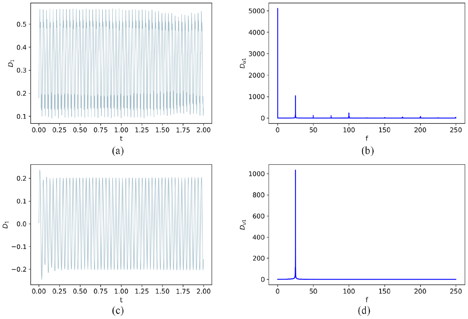
Pre-processing of the measured signals. (a) Raw signal measured at disk 1 node; (b) Frequency spectrum of (a) without normality; (c) Filtered signal and (d) Frequency spectrum of (c) without normality.

Identification of the unbalanced forces

In this subsection, two approaches are applied to identify the equivalent imbalance masses on selected correction planes. The first one is ICM and for the second approach, the unsupervised deep learning balancing method is adopted. In both approaches, #2 and #5 disks are selected as correction planes. The radium of balancing groove are 40 mm on each disk.

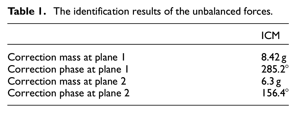
For ICM, the responses from #1 to #6 nodes are all used to calculate the influence parameters. After two times of weight trail processes, the correction mass and angle can be get by least square method. The result are listed in Table 1.

Table 1.

The identification results of the unbalanced forces.

	ICM
Correction mass at plane 1	8.42 g
Correction phase at plane 1	285.2°
Correction mass at plane 2	6.3 g
Correction phase at plane 2	156.4°

For the unsupervised deep learning method, not only the pre-processed raw signals measured from #1 to #6 nodes, but also the forces measured by dynamic force sensors are used for training the network. The displacements are measured directly. The velocities and accelerations are get by deriving the displacement numerically. The bearing forces can be estimated by solving equation (4) with the reference of measured force signals algebraically.

The raw data is collected for a time period of 15 s with sampling frequency of 500 Hz. Here, the sample’s length is set to 1. That means the training data will have a size of 7500. Then, the joint configurations $(q, \overset{\cdot}{q}, \overset{\cdot\cdot}{q})$ took out from the training data-set will be input to the network described in Figure 1(b). And the $τ_{s}$ -dimensional outputs are compared with the $τ_{sm}$ by loss function for parameters update. Mean squared error (MSE) of $τ_{sm}$ and $τ_{s}$ is used as the optimization objection. Mini-batch of 128 and Adam optimizer are applied during the training process.

After 2000 epochs, the prediction values of the unbalanced forces are shown as black lines in Figure 6. As the unbalanced force is assumed to be harmonic type, the first guess (light blue lines in Figure 6) follows the rule of

g_std * \cos (Ω t + g_pha) + g_mean

Figure 6.

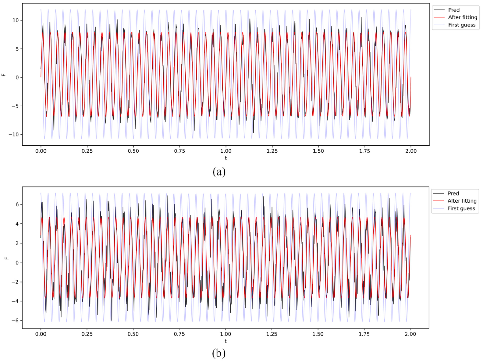
The prediction results of the unbalanced forces and their harmonic fits: (a) the results at correction plane 1 and (b) the results at correction plane 2.

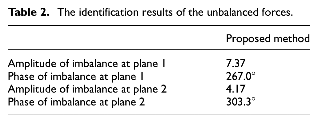
where $g_mean = Mean (data)$ , $g_std = \frac{3 \sqrt{2}}{2} Std (data)$ and $g_pha = 0$ . The least square method then is used to fit the amplitude and the phase of the unbalanced forces. The identification results (red lines in Figure 6) can be used to balance the rotor. The identification results are listed in Table 2.

Table 2.

The identification results of the unbalanced forces.

	Proposed method
Amplitude of imbalance at plane 1	7.37
Phase of imbalance at plane 1	267.0°
Amplitude of imbalance at plane 2	4.17
Phase of imbalance at plane 2	303.3°

Experimental results after balancing

Based on the identification results of the amplitudes and the phases of the unbalanced forces by ICM and UDL, the experimental rotor system with imbalances established can be balanced. The balanced effects are illustrated in Figure 7. In Figure 7, light blue lines indicate the responses of the unbalanced rotor system after pre-processing. The black broken lines give the responses of the balanced rotor after balancing by ICM. The red curves are the responses of the rotor balanced by UDL. From the comparisons, we could find that both ICM and UDL can balance the rotor and the amplitude of the responses reduce significantly after balancing. Comparing these two methods, the results by UDL are better than ICM. The reason for the results is that the ICM is a linear method, which assumes that the relationship between the response and input is linear. This assumption would lead to error when the effect of the nonlinear factor of the system is huge. However, the mapping function used in UDL is nonlinear, which dealt with the nonlinear factor induced by the ball bearings better. Meanwhile, it is noted that when balancing by UDL, no extra weight trail processes are needed. The comparison results indicate that the UDL is effective and costless.

Figure 7.

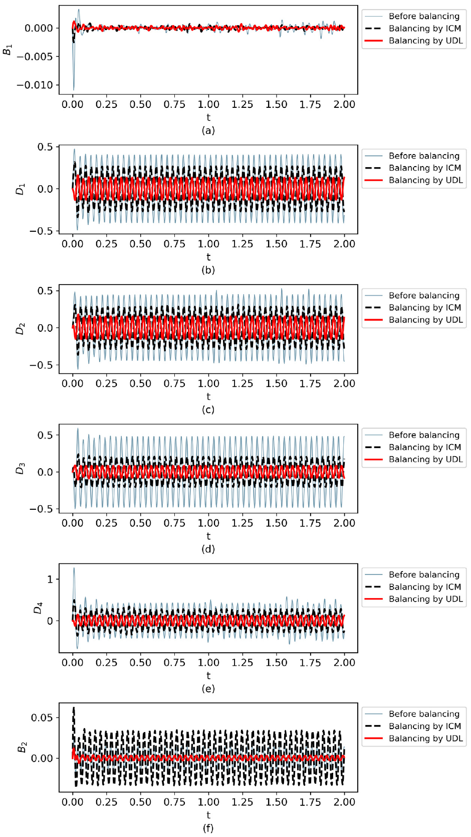
Balancing effects on (a) node 1, (b) node 2, (c) node 3, (d) node 4, (e) node 5, and (f) node 6 by ICM and UDL.

Discussions and conclusions

An experiment rig of a rotor to investigate rotor dynamics and balancing technology is set up. Two balancing approaches are conducted. One is the classical ICM and the other approach for rotor balancing uses unsupervised deep learning. In the deep network based method, the joint configurations of the general displacements, velocities and accelerations are used as input and estimated bearing forces are set to be labels. Based on the rig, two rotor balancing experiments by ICM and UDL are conducted. The results from both experiments prove that the design of the rig is reasonable and can be used for further analysis of rotor dynamics and validation of control schemes. Meanwhile, the proposed method which uses unsupervised deep learning technology is proved to be costless and performs well.

It’s noting that in the proposed network and training process, there are many parameters that can be optimized to achieve better performances. For instance, the physical prior layer can be added to neural network module to introduce the physical meaning of the mechanical system. The size of a single sample can be enlarged during data pre-processing so that more historic information could be involved. And in practical operations, how to add or reduce the trail weights in proper positions is an important challenge in further rotor design.

Footnotes

Declaration of conflicting interests

The author(s) declared no potential conflicts of interest with respect to the research, authorship, and/or publication of this article.

Funding

The author(s) disclosed receipt of the following financial support for the research, authorship, and/or publication of this article: This work was supported by the National Natural Science Foundation of China (Grant Nos. 12102234, 11902184, 11502161).

ORCID iDs

Shun Zhong

References

Yao

Yang

, et al. Balancing optimization of a multiple speeds flexible rotor. J Sound Vib 2020; 480: 115405.

Cao

, et al. Calibration of a hub dynamic balancing machine based on the least squares method and systematic error analysis. IEEE Access 2020; 8: 178746–178754.

Ranjan

Tiwari

On-site high-speed balancing of flexible rotor-bearing system using virtual trial unbalances at slow run. Int J Mech Sci 2020; 183: 105786.

Zhang

Online measuring and estimating methods for the unbalancing vector of thin-disc workpiece based on the adaptive influence coefficient. J Vib Control 2021; 27: 1753–1764.

Bishop

RED

Gladwell

GML

. The vibration and balancing of an unbalanced flexible rotor. J Mech Eng Sci 1959; 1(1): 66–77.

Bishop

RED

Parkinson

. On the use of balancing machines for flexible rotors. J Manuf Sci Eng 1972; 94(2): 561–572.

Goodman

TP.

A least-squares method for computing balance corrections. J Manuf Sci Eng 1964; 86(3): 273–277.

Lund

Tonnesen

Analysis and experiments on multi-plane balancing of a flexible rotor. J Manuf Sci Eng 1972; 94(1): 233–242.

Untaroiu

Allaire

Foiles

WC.

Balancing of flexible rotors using convex optimization techniques: optimum min-max LMI influence coeﬃcient balancing. J Vib Acoust 2008; 130(2): 021006.

10.

Wang

SQP algorithms in balancing rotating machinery. Mech Syst Signal Process 2007; 21(3): 1469–1478.

11.

Messager

Pyrz

Discrete optimization of rigid rotor balancing. J Mech Sci Technol 2013; 27(8): 2231–2236.

12.

Kang

Lin

Chang

, et al. Optimal balancing of flexible rotors by minimizing the condition number of influence coefficients. Mech Mach Theory 2008; 43(7): 891–908.

13.

Lin

Allaire

PE.

Robust optimal balancing of high-speed machinery using convex optimization. J Vib Acoust 2008; 130(3): 031008.

14.

Tresser

Dolev

Bucher

Dynamic balancing of super-critical rotating structures using slow-speed data via parametric excitation. J Sound Vib 2018; 415: 59–77.

15.

Khulief

Oke

Mohiuddin

MA.

Modally tuned influence coefficients for low-speed balancing of flexible rotors. J Vib Acoust 2014; 136: 136–142.

16.

Deepthikumar

Sekhar

Srikanthan

MR.

Modal balancing of flexible rotors with bow and distributed unbalance. J Sound Vib 2013; 332(24): 6216–6233.

17.

Villafane Saldarriaga

Steffen

Der Hagopian

, et al. On the balancing of flexible rotating machines by using an inverse problem approach. J Vib Control 2011; 17(7): 1021–1033.

18.

Han

DJ.

Generalized modal balancing for non-isotropic rotor systems. Mech Syst Signal Process 2007; 21(5): 2137–2160.

19.

Zhao

Ren

Deng

, et al. A transient characteristic-based balancing method of rotor system without trail weights. Mech Syst Signal Process 2021; 148: 107117.

20.

Zheng

Liu

Balancing of flexible rotors without trial weights based on finite element modal analysis. J Vib Control 2013; 19(3): 461–470.

21.

Zhang

, et al. The whole-beat correlation method for the identification of an unbalance response of a dual-rotor system with a slight rotating speed difference. Mech Syst Signal Process 2011; 25(5): 1667–1673.

22.

Zhang

Wang

Jin

, et al. Non-whole beat correlation method for the identification of an unbalance response of a dual-rotor system with a slight rotating speed difference. Mech Syst Signal Process 2013; 39(1–2): 452–460.

23.

Yue

Ren

Yang

, et al. Unbalance identification of speed-variant rotary machinery without phase angle measurement. Shock Vib 2015; 2015: 1–11.

24.

Mao

Lei

, et al. A new adaptive proportional-integral control strategy for rotor active balancing systems during acceleration. Mech Mach Theory 2019; 136: 105–121.

25.

Peng

Deng

, et al. Field dynamic balancing for active magnetic bearings supporting rigid rotor shaft based on extended state observer. Mech Syst Signal Process 2021; 158: 107801.

26.

Zheng

Wang

Rotor balancing for magnetically levitated tmps integrated with vibration self-sensing of magnetic bearings. IEEE/ASME Trans Mechatron 2021; 26: 3031–3039.

27.

Ait Ben Ahmed

Touache

El Hakimi

, et al. A new hybrid method for rigid and flexible rotor balancing without phase response measurements. Aust J Mech Eng 2020; 1–13. doi: 10.1080/14484846.2020.1842616.

28.

Zhong

Chen

, et al. A novel balancing method for rotor using unsupervised deep learning. Shock Vib 2021; 2021: 1–9.

29.

Lutter

Listmann

Peters

Deep Lagrangian networks for end-to-end learning of energy-based control for under-actuated systems. arXiv preprint, arXiv:1907.04489, 2019.

30.

Ting

Mistry

Peters

, et al. A Bayesian approach to nonlinear parameter identiﬁcation for rigid body dynamics. In: Sukhatme

G. S.

Schaal

Burgard

Fox

(Eds.), Robotics: science and systems, Philadelphia, PA, 16–19 August, 2006, pp.32–39. Cambridge, MA: MIT Press.

31.

Haruno

Wolpert

Kawato

Mosaic model for sensorimotor learning and control. Neural Comput 2001; 13(10): 2201–2220.

32.

Calinon

D’halluin

Sauser

, et al. Learning and reproduction of gestures by imitation. IEEE Robot Autom Mag 2010; 17(2): 44–54.

33.

Ledezma

Haddadin

First-order-principles-based constructive network topologies: An application to robot inverse dynamics. In:2017 IEEE-RAS 17th international conference on humanoid robotics (Humanoids), 2017, pp.438–445. New York, NY: IEEE.

On experiments of a novel unsupervised deep learning based rotor balancing method

Abstract

Keywords

Introduction

Methodology

Set up of experimental rig

Experimental results analysis

Experimental results before balancing

Identification of the unbalanced forces

Experimental results after balancing

Discussions and conclusions

Footnotes

Declaration of conflicting interests

Funding

ORCID iDs

References