Unsupervised learning trajectory anomaly detection algorithm based on deep representation

Abstract

Without ground-truth data, trajectory anomaly detection is a hard work and the result lacks of interpretability. Moreover, in most current methods, trajectories are represented by geometric features or their low-dimensional linear combination, and some hidden features and high-dimensional combined features cannot be found efficiently. Meanwhile, traditional methods still cannot get rid of the limitation of space attributes. Therefore, a novel trajectory anomaly detection algorithm is present in this article. Unsupervised learning mechanism is used to overcome nonground-truth problem and deep representation method is used to represent trajectories in a comprehensive way. First, each trajectory is partitioned into segments according to its open angles, then the shallow features at each point of a segment are extracted and. In this way, each segment is represented as a feature sequence. Second, shallow features are integrated into auto-encoder-based deep feature fusion model, and the fusion feature sequences can be extracted. Third, these fused feature sequences are grouped into different clusters using a unsupervised clustering algorithm, and then segments which quite differ from others are detected as anomalies. Finally, comprehensive experiments are conducted on both synthetic and real data sets, which demonstrate the efficiency of our work.

Introduction

With the continuous development and application of positioning equipment, such as global position system (GPS), Wi-Fi as well as wireless sensor network (WSN), a large volume of moving objects can be tracked with their trajectory data stored in the database. It has been a hot topic of analyzing and extracting knowledge from these data. Hawkins ¹ gave the definition of outlier as follows: an observation deviates greatly from others and arouses suspicion that it was generated by a different mechanism. Trajectory anomaly detection^2,3 is an important research branch in the field of trajectory data mining. And its task is to discover trajectories or their segments which differ substantially from or are inconsistent with the remaining set. As for trajectory anomaly, an outlier means a data object that is grossly different from or inconsistent with the remaining set of data. ⁴ Traditional anomaly detection algorithms mainly consist of distance-based algorithms^5–7 and density-based algorithms,^8,9 but unsupervised methods are rarely used. The distance-based algorithm mostly judges whether the trajectory is anomaly or not according to the space distance of the trajectory. Due to limitations in space distance comparison, the trajectory with the same characteristics but far distance may be detected as an exception, which will affect the accuracy of the trajectory anomaly detection. The density-based algorithm is essentially the extension of distance algorithm, which cannot fundamentally eliminate the limitations of distance-based trajectory anomaly detection algorithm.

In the traditional methods of trajectory anomaly detection, the trajectory is usually represented by hand extracted geometric features or low-dimensional linear combination of geometric features. These representation methods cannot find some hidden features or high-dimensional composite features. For example, Figure 1 shows the shape, angle change, distance change, and speed change of trajectory, respectively. By analyzing the internal characteristic attributes of trajectory such as angle, speed, and distance, it is found that the change degree is different. It can be seen that only measuring the linear combination of a certain geometric feature or a simple geometric feature is not enough to comprehensively reflect the movement trend of the trajectory. It is difficult to comprehensively describe the movement mode of the moving object’s trajectory. Therefore, error may exist in the result of anomaly detection because of incomplete feature extraction and incomplete representation of trajectory feature sequence.

Figure 1.

An example of trajectory structural features: (a) shape of trajectory, (b) angle change, (c) distance change, and (d) velocity change.

In view of the shortcomings of existing research methods, this article proposes an unsupervised learning trajectory anomaly detection algorithm based on deep representation (TAD-FM). Through the transformation and processing of GPS data, the trajectory is described comprehensively with deep characteristics. Compared with algorithms based on distance and density, the deep feature fusion model based on auto-encoder is proposed in this article, which transforms the geometric feature representation of trajectory into sequence pattern, represents trajectory by feature sequence, and desalinates the spatial attribute of trajectory itself. Therefore, the limitation of using spatial distance to judge anomalies is fundamentally solved. At the same time, from the perspective of fully exploring the characteristics of the trajectory, the low-dimensional shallow features and the high-dimensional deep features of the trajectory are integrated to describe the trajectory comprehensively. So as to characterize the overall trajectory features according to the description sequence to detect the trajectory anomaly.

The main framework of this article is given in Figure 2 with parts of ideas borrowing from Chen et al. ¹⁰ GPS trajectory data can be obtained from a variety of positioning devices. The original GPS trajectory data are a three-dimensional (3D) data composed of longitude, latitude, and time. In the trajectory data division stage, the trajectory is divided into segments according to the open angle. In the stage of deep feature extraction, the trajectory segment is transformed into shallow feature sequence first, and then the shallow feature sequence is put into the deep feature fusion model based on auto-encoder to obtain the deep feature sequence representation of trajectory segment, that is, the original GPS data of trajectory segment are transformed into the fusion feature sequence. In the clustering stage, in order to obtain the trajectory segments of different motion modes, the density-based spatial clustering of applications with noise (DBSCAN) algorithm is used to cluster by measuring the cosine distance between fusion feature sequences. In the phase of anomaly detection, the anomaly trajectory segments are extracted by comparing the cosine similarity between the fusion feature sequences, and then consider the proportion of the anomaly trajectory segments in the overall trajectory, finally detect the anomaly trajectory.

Figure 2.

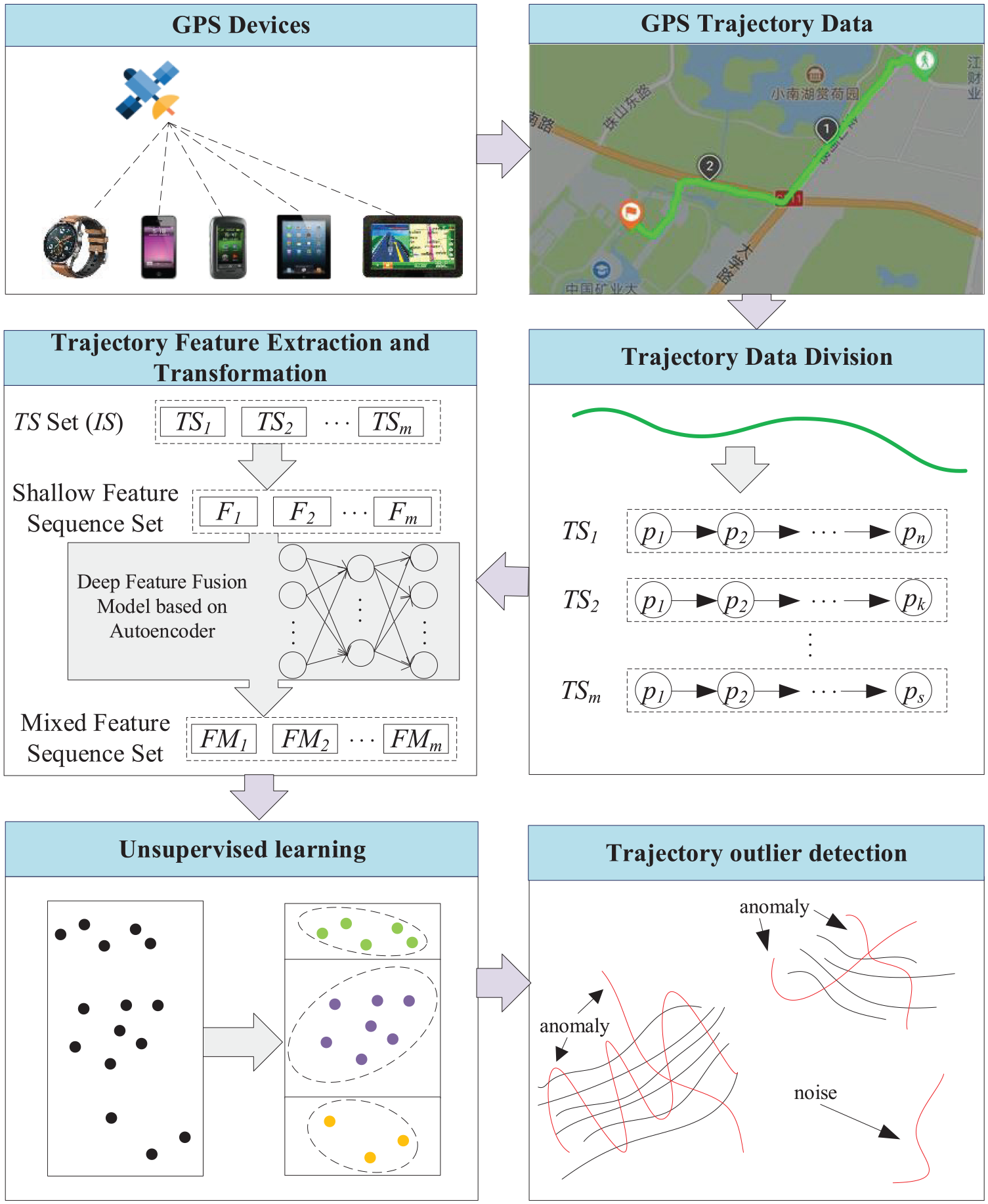
The framework of this article.

The main contributions of this article are as follows:

1. On the basis of the idea of deep embedding, a deep feature fusion model based on auto-encoder is proposed to reduce human intervention, extract high-dimensional combined features of trajectory, transform the geometric feature sequence of trajectory into the mixed feature sequence of high-dimensional non-linear representation, and describe the trajectory comprehensively.

2. The geometric representation of the trajectory is transformed into a sequential pattern. The limitation of using spatial distance to judge the anomaly is fundamentally solved using the way of feature sequence to represent the trajectory and desalinate the spatial attribute of the trajectory itself.

3. Experiments based on multiple data sets show that the algorithm proposed in this article can discover the anomaly trajectory, which proves the effectiveness and feasibility of the algorithm.

The organization structure of this article is as follows. In section “Related work,” the related work is described. In section “Trajectory representation,” the method of trajectory division is introduced. In section “Feature extraction and transformation,” the deep feature fusion model based on auto-encoder is proposed to describe how to extract and transform the features from the divided trajectory segments. In section “Unsupervised learning clustering,” the multi-category clustering method based on unsupervised learning is introduced. In section “Trajectory outlier detection,” the method of trajectory anomaly detection is described in detail. In section “Experimental analysis,” the algorithm is evaluated by experiments. In section “Some real application scenarios,” some typical application scenarios are discussed. In section “Conclusion,” the full text is summarized, and the future research direction is pointed out.

Related work

Trajectory anomaly detection

Distance-based algorithm

Knorr et al. ⁷ not only regarded the trajectory as a series of points but also transformed the trajectory into a feature sequence of position, direction, and speed. By comparing the distance, the trajectory anomaly was detected. However, this method only compares the overall characteristics of the trajectory while ignores the local characteristics. As the trajectory grows, the problems exposed by this method become more and more obvious. In order to solve the problem caused by comparing the whole trajectory, Lee et al. ⁵ proposed the density-based trajectory outlier detection (TRAOD) algorithm. The TRAOD algorithm consists of two steps: division and detection. In the division step, the trajectory is divided into several segments, which are represented by the line segments connected by two sampling points. In the detection step, the distance between the line segments is used to measure its matching, so as to detect the trajectory anomaly. This method solves the problem of complex trajectory anomaly detection, but only by describing the trajectory segment as a directed segment composed of the start and end points, the characteristics of the trajectory itself are inevitably ignored. Yuan et al. ⁶ put forward the trajectory structure framework and introduced it into the trajectory anomaly detection. By considering the internal characteristics of the trajectory, the accuracy of the analysis is improved, so as to avoid the problem of only comparing the spatial shape of the trajectory. However, due to the different importance of each internal feature of the trajectory, subjective weight will interfere with the results, thereby affecting the accuracy of anomaly detection. Most distance-based algorithms judge whether the trajectory is anomaly or not according to the space distance of the trajectory. Because of the limitation of space distance comparison, it is inevitable that the trajectory with the same characteristics but a long distance is detected as an exception, which affects the accuracy of the trajectory anomaly detection.

Density-based algorithm

Breunig et al. ⁸ used local anomaly factor (LOF) to determine whether the trajectory is anomaly, but a large number of neighbor queries are required to calculate LOF, so the cost of calculation is very high. ¹¹ Liu et al. ⁹ introduced the concept of trajectory density and proposed density-based trajectory outlier detection (DBTOD) algorithm to make up for the shortcomings that TRAOD algorithm cannot detect local and dense trajectories. The density between trajectories is calculated by distance, so the density-based algorithm is essentially an extension of distance-based algorithm, which cannot fundamentally solve the limitations of the distance-based algorithm.

Embedding

Sutskever et al. ¹² first proposed the method of sequence-to-sequence auto-encoder for machine translation. Chen et al. ¹⁰ used auto-encoder fusing a variety of different features to get more semantical and discriminative context representation in the latent space, so as to analyze the taxi destination. Liu et al. ¹³ used embedding method for real-time personalized search and similar product list recommendation. Dong et al. ¹⁴ proposed a novel Auto-encoder Regularized deep neural Network (ARNet) and a trip encoding framework trip2vec to learn drivers’ driving styles directly from GPS records, by combining supervised and unsupervised feature learning in a unified architecture. Embedding method is widely used. Through the analysis of the above methods, this article applies the embedding method to trajectory anomaly detection. Beritelli et al. ¹⁵ proposed a radial basis probabilistic neural network to classify non-linear and unstable data. The implemented method has been devised in order to slowly increase, during training, the generalization capabilities of a radial basis probabilistic neural network classifier as well as preventing it from over-generalization and the consequent lack of resulting classification performances.

Trajectory representation

The temporal distance between two consecutive points in the same trajectory is relatively small (with respect to the mobility phenomenon under consideration). In this view, the trajectory is simply a sequence of relatively close in time ordered points. ¹⁶ Generally speaking, the segmentation task splits a sequence of data points, in a series of disjoint subsequences consisting of points that are homogeneous with respect to some criteria.^17,18 Therefore, this article uses the divided trajectory segment as the basic unit of analysis.

Maike et al. ¹⁹ defined the segmentation problem as follows: to split a high-sampling rate trajectory into a minimum number of segments such that the movement characteristic inside each segment is uniform in some sense. The purpose of dividing a trajectory into segments is that trajectory segments contain part of the original trajectory data and hidden information, so they can be more flexible to combine and describe trajectory. ²⁰ The key of trajectory division is to find some key points that can divide the trajectory into multiple smooth trajectory segments. Through the key points to divide the trajectory, it can effectively divide the trajectory segments that retain trajectory characteristics and are relatively smooth. If the trajectory is not divided and the whole trajectory is taken as the input data to extract features, some key information will be ignored. Therefore, compared with not dividing the trajectory, the trajectory division can grasp the internal characteristics of the trajectory. At the same time, keeping the internal characteristics of the trajectory without losing is conducive to anomaly detection. The definition of trajectory and open angle is given here.

Definition 1

Trajectory: ²¹ Given a trajectory set I = {T₁, T₂, T₃, …, T_n} composed of a series of trajectories, where each trajectory is a series of multi-dimensional points in chronological order, expressed as T_i = {p₁, p₂, p₃, …, p_m} (1 ≤ i ≤ n). p_j (1 ≤ j ≤ m) is a point in the trajectory, expressed as <lat_j, lon_j, time_j>. TS_l = {p_c1, p_c2, p_c3, …, p_ck} (1 ≤ c1 < c2 < c3 < … < ck ≤ m) is called a trajectory segment of T_i, and the set of all trajectory segments is called trajectory segment set, which is expressed as IS = {TS₁, TS₂, TS₃, …, TS_h }.

Definition 2

Open angle: ²² Three points {P₁, P₂, P₃} in the trajectory segment form an angle α less than π. If α is less than the given threshold value ω, then α is called the open angle. The corresponding point of α is the key point. α is calculated by equation (1). As shown in Figure 3, if α < ω, P₂ is the key point and α is the open angle

$$\alpha =\arccos \frac{a^2+b^2-c^2}{2\mathrm{ab}}$$

(1)

Figure 3.

The open angle of trajectory.

Using the two-pass corner detection algorithm, ²¹ all the points are scanned and the open angle are calculated according to Definition 2, so as to determine the key points of the trajectory finally. The method can accurately divide the trajectory into each smooth trajectory segment with consistent overall movement trend according to the key points.

In order to describe the process of track division more clearly, a simple example is used to illustrate the trajectory division. Figure 4 shows the schematic diagram of trajectory segment division. According to Definition 2, α₁ is calculated as 119°, α₂ as 128°, and the threshold ω is set as 125°. It can be seen that α₁ is less than the threshold value, α₂ is greater than the threshold value, then α₁ is the open angle, P₁ is the key point, and the trajectory is divided into two trajectory segments at P₁.

Figure 4.

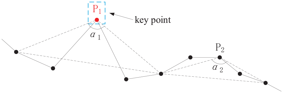
Trajectory segmentation.

Feature extraction and transformation

Deep neural networks have been proved powerful in learning from speech data,^23,24 text data, ²⁵ and image data. ²⁶ Trajectory data are similar to language and text data, and these are also a kind of time series data. However, according to Definition 1, trajectory data are 3D data composed of two-dimensional (2D) coordinates and timestamps. Empirical studies showed that simply treating raw trajectory data as 3D signal inputs for either traditional machine learning or deep learning algorithms just does not work. ²⁷ Therefore, in order to make the trajectory data suitable for the deep neural network algorithm, it is necessary to extract the trajectory features with stronger semantic expression from the original trajectory data. The original trajectory data are represented by feature sequence.

As shown in Figure 5, the core of feature extraction and transformation is divided into two steps. First, the geometric features are extracted from several indefinite length original trajectory segments and transformed into fixed length shallow feature sequence F through dimension expansion. Second, the deep feature fusion model based on auto-encoder is used to transform shallow feature sequence into mixed feature sequence FM, that is, shallow feature sequence F is spliced with deep trajectory feature sequence FD to get mixed feature sequence FM.

Figure 5.

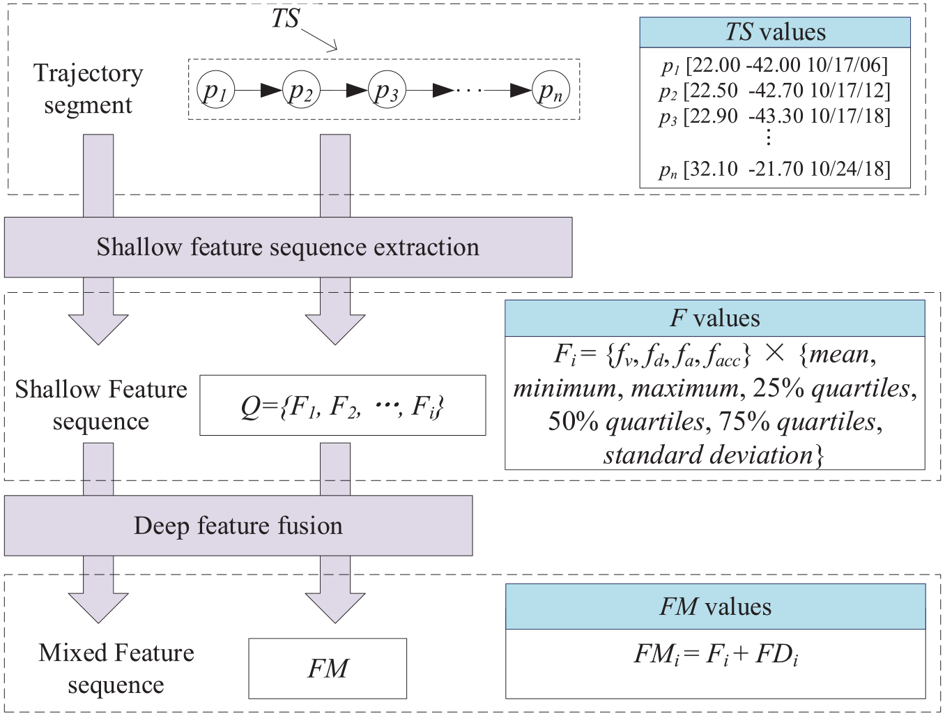
Feature extraction and conversion.

Shallow feature sequence extraction

The trajectory segment TS contains rich information, from which a variety of information can be extracted to represent the movement trend and structural features of the trajectory segment. In this article, four representative geometric features are extracted from the trajectory segment: velocity change f_v, distance change f_d, angle change f_a, and acceleration change f_acc. However, GPS data may have errors in recording, and the influence of different degrees of change in the same feature on trajectory segments is different. In order to reduce the inaccuracy of feature extraction caused by possible data errors, so that the relevant features can be represented in a more detailed way, the original geometric features need to be expanded.

Definition 3

Shallow feature sequence: A frame encoding statistics of the basic features is called the shallow feature of the trajectory. The set Q composed of n shallow trajectory feature sequences is called shallow feature sequence set, which is expressed as Q = {F₁, F₂, F₃, …, F_n}. Each shallow feature sequence F_i represents a trajectory segment TS_i, 1 ≤ i ≤ n.

Dimension expansion requires calculating mean, minimum, maximum, 25%, 50%, and 75% quartiles, and standard deviation of each trajectory segment feature. ¹ The calculated results are the shallow feature sequences of each trajectory segment. According to Definition 3, this article analyzes the velocity variation f_v, distance variation f_d, angle variation f_a, and acceleration variation f_acc of the trajectory. The shallow feature sequence F is expressed as F = {f_v, f_d, f_a, f_acc} ×{mean, minimum, maximum, 25% quartiles, 50% quartiles, 75% quartiles, standard deviation}. Obviously, in this article, the shallow feature sequence F is a 28(4×7) dimensional feature sequence. The shallow feature sequence can reflect the trajectory segment intuitively and quantify the original GPS trajectory data at the same time. The trajectory segment set is represented by the shallow feature sequence set Q, which is convenient for later analysis and processing.

Deep feature fusion

A deep feature fusion model based on auto-encoder is proposed. The shallow feature sequence is transformed into deep feature sequence using the model, and the shallow feature sequence and deep feature sequence are spliced into mixed feature sequence, so that the features of trajectory segments can be represented comprehensively from deep and shallow aspects.

Auto-encoder

By analyzing the trajectory segments represented by the intuitionistic feature sequences, we can find the anomalies. However, the shallow feature sequence is only the feature representation of low-dimensional trajectory segments, which will limit the performance of machine learning algorithm. The typical problem is that the potential feature information and the association between different types of combined features cannot be found. ²² Therefore, this article uses auto-encoder^10,28 to solve this problem. Auto-encoder belongs to the embedding method, which is an unsupervised artificial neural network. After many training, it can capture the most significant features in the input data.

Figure 6 shows a three-layer auto-encoder model. L₁ is the input layer, L₂ is the hidden layer, and L₃ is the output layer. Among them, the input layer L₁ and the hidden layer L₂ constitute the encoder, which are responsible for extracting potential features. The hidden layer L₂ and the output layer L₃ constitute the decoder, which are responsible for reconstructing the input data from the hidden layer. The data in input layer L₁, hidden layer L₂, and output layer L₃ are represented by x, h, and y ( $x,y\in [0,1{]}^n$ , $h\in [0,1{]}^m$ ). W is the weight matrix ( $W\in R^{m\times n}$ ), b₁ is the offset of input layer L₁ ( $b_1\in R^m$ ), and b₂ is the offset of hidden layer L₂ ( $b_2\in R^n$ ).

Figure 6.

The process of auto-encoder.

The value h in hidden layer L₂ and the value y in output layer L₃ are calculated by equations (2) and (3), where $\sigma (·)$ represents sigmod activation function

$$h=f(x)=\sigma (\mathrm{Wx}+b_1)$$

(2)

$$y=g(h)=\sigma (W^{T}h+b_2)$$

(3)

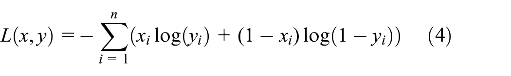
The purpose of using auto-encoder is to extract the significant high semantic features of the original data from the hidden layer; at the same time, it has the function of reducing dimension and noise. In order to make the learned hidden layer meaningful, the data output by the encoder needs to enter the decoder again for decoding. Through repeated iterations, the input and output parameters are updated to make the value of y and x close, that is, the target optimization function of $y=F_{w,b}(x)\approx x$ is learned from the encoder. The target optimization function can be represented by the reconstruction error function L(x, y), as shown in equation (4). According to the reconstruction error function, loss function can be obtained, which is calculated by equation (5)

$$L(x,y)=-\sum _{i=1}^n(x_i\log \left(y_i\right)+(1-x_i)\log (1-y_i))$$

(4)

$$\mathrm{Loss}=\sum _{x\in Q}L(x,g(f(x)))$$

(5)

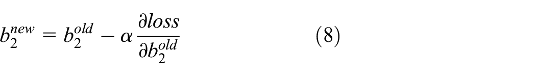
The updating methods of weight matrix W and offset quantities b₁ and b₂ are shown in equations (6)–(8)

$$W^{\mathrm{new}}=W^{\mathrm{old}}-\alpha \frac{\partial \mathrm{loss}}{\partial W^{\mathrm{old}}}$$

(6)

$$b_1^{\mathrm{new}}=b_1^{\mathrm{old}}-\alpha \frac{\partial \mathrm{loss}}{\partial b_1^{\mathrm{old}}}$$

(7)

$$b_2^{\mathrm{new}}=b_2^{\mathrm{old}}-\alpha \frac{\partial \mathrm{loss}}{\partial b_2^{\mathrm{old}}}$$

(8)

In this article, in order to make the results more practical, only the vectors in the hidden layer L₂ represented by the high-dimensional feature sequence after feature compression, that is, after feature reconstruction, are selected as the output results of the auto-encoder.

Mixed feature sequence transformation

In this section, the deep feature fusion model based on auto-encoder is introduced in detail. In order to express conveniently, the definition of deep feature sequence and mixed feature sequence is introduced first.

Definition 4

Deep trajectory feature sequence: The deep trajectory feature sequence FD is obtained by depth representation of the shallow trajectory feature sequence F. The set QD composed of n deep trajectory feature sequences is called deep feature sequence set, which is expressed as QD = {FD₁, FD₂, FD₃, …, FD_n}. Among them, each deep feature sequence FD_i represents a trajectory segment TS_i and is also the deep representation of the shallow feature sequence F_i, 1 ≤ i ≤ n.

Definition 5

Mixed feature sequence: The feature sequence F_i and the deep feature sequence FD_i, which represent the same trajectory segment TS_i, are spliced, and the spliced sequence is expressed in high-dimensional depth. The result sequence is the mixed feature sequence FM_i. The set of all mixed feature sequences is called mixed feature sequence set MD, which is expressed as MD = {FM₁, FM₂, FM₃, …, FM_n}, 1 ≤ i ≤ n.

The shallow feature sequence and the deep feature sequence can express the shallow and deep features, respectively. Using the deep feature fusion model based on auto-encoder, the shallow feature sequence and the deep feature sequence are transformed into the mixed feature sequence, which not only considers the detail information of the shallow feature but also combines the semantic information of the deep feature. So, the shallow and deep features can be highlighted at the same time.

Figure 7 shows the deep feature fusion model based on auto-encoder. By inputting the shallow feature sequence into auto-encoder 1, we can get the deep feature sequence shown in Definition 4. Using the deep feature sequence FD to express the trajectory segment in a higher dimension, we can capture the relationship between the potential valuable feature information in the trajectory segment and a variety of non-linear combined features. Then, the deep feature sequence and the shallow feature sequence are spliced into the auto-encoder 2. The mixed feature sequence shown in Definition 5 can be obtained. The weight and offset of the feature sequence put into the auto-encoder are calculated by equations (6)–(8). Using the fusion feature sequence FM, the trajectory segments are described comprehensively from the two aspects of the shallow feature and the deep feature.

Figure 7.

Feature integration.

Obviously, in this article, the dimension of input shallow feature sequence F is 28. In view of the consumption of computing time and the size of reconstruction error, the dimensions of hidden layer L₂ of auto-encoder 1 and auto-encoder 2 are set to 10 and 15, respectively. When the 28-dimensional F input model, the 10-dimensional FD is obtained through auto-encoder 1. Then, spliced FD with F and sent to auto-encoder 2. Finally, the 15-dimensional FM is obtained.

Unsupervised learning clustering

The purpose of unsupervised learning–based multi-category clustering is to divide different types of trajectory segments into different clusters. The trajectory segments that need to be detected should exist in the same neighborhood, that is, the same cluster with similar motion mode, rather than all the trajectory segments in the set. This is conducive to reducing the complexity of the algorithm and also has practical significance.

However, traditional clustering methods are often based on hand-crafted features. These features have limited capacity and cannot dynamically adjust to capture the prior distribution. ²⁹ Therefore, this article uses the features processed by the deep feature fusion model based on auto-encoder to cluster and breaks through the limitation of manual feature extraction for the overall representation of trajectory.

Definition 6

Cosine similarity: The method to evaluate the similarity of two mixed feature sequences by calculating the cosine value of the angle between them is called cosine similarity. Equation (9) shows the cosine similarity of the mixed feature sequence FM_i and FM_j, 1 ≤ i, j ≤ n

$$s_{\mathrm{ij}}=\frac{F{M}_i·F{M}_j}{F{M}_{i}F{M}_j}$$

(9)

The purpose of using cosine similarity to measure distance is that most of the current trajectory clustering algorithms rely on the spatiotemporal similarity measurement of trajectory. They cannot cluster trajectories with similar characteristics that exist in different spatiotemporal regions. In this article, the mixed feature sequence is used to represent the trajectory segments, and all the trajectory segments are described as space vectors of common starting point. The cosine similarity is used to measure the distance between them. The vectors pointing to a certain range are grouped into one category, that is, the trajectory segments with similar features are grouped into one cluster, which breaks through the limitation of space-time.

In this article, the density-based clustering algorithm DBSCAN ³⁰ is used to cluster, and the cosine similarity shown in Definition 6 is used to measure the distance. DBSCAN can find clusters of any shape and can find irregular clusters without knowing the number of clusters in advance. The unsupervised trajectory anomaly detection algorithm proposed in this article has no clear attribute label for the attribute type of trajectory, and the subjective specified clustering number will affect the classification of trajectory. Therefore, the DBSCAN algorithm has a high applicability.

Definition 7

ε-neighborhood: If the mixed feature sequence FM_i and FM_j are in MD and the cosine similarity does not exceed the nearest neighbor threshold ε, then the ε nearest neighbor of the mixed feature sequence FM_i is expressed as N_ε(FM_i), which is expressed by equation (10), where $s_{\mathrm{ij}}(F{M}_i,F{M}_j)$ indicates the cosine similarity between FM_i and FM_j

$$N_{\epsilon }\left(F{M}_i\right)=\{F{M}_j\in \mathrm{MD}\cap i\ne j|s_{\mathrm{ij}}(F{M}_i,F{M}_j)\le \epsilon \}$$

(10)

Definition 8

Core sequence: For any mixed feature sequence $F{M}_i\in \mathrm{MD}$ , if $\left|N_{\epsilon }\left(F{M}_i\right)\right|\ge \mathrm{MinPts}$ , FM_i is the core sequence.

Definition 9

Directly density-reachable: If $F{M}_i\in N_{\epsilon }(F{M}_j)$ and $|N_{\epsilon }(F{M}_j)|\ge \mathrm{MinPts}$ , FM_i is said to be directly density-reachable by FM_j.

Definition 10

Density-reachable: If there is a series of mixed feature sequences FM_i, FM_i+1, …, FM_j, and FM_j−1, where FM_p and FM_p+1 are directly density-reachable, then FM_i is said to be density-reachable by FM_j. Density-reachable does not have symmetry.

Definition 11

Cluster: If a non-empty set C satisfies the following two conditions, then it is called cluster

1. Connectivity: For $\forall F{M}_i,F{M}_j\in C$ , FM_i and FM_j are density connected.

2. Maximality: for $\forall F{M}_i,F{M}_j$ , if $F{M}_i\in C$ and FM_j can be reached by FM_i density, then there is $F{M}_j\in C$ .

Definition 12

Noise: In the cluster set Cl = {C₁, C₂, C₃, …, Cm_m}, the mixed feature sequence FM_k that exists in the mixed feature sequence set MD but does not belong to any clustering C_i is called noise, that is, $\mathrm{noise}=\{F{M}_k\in \mathrm{MD}|F{M}_k\notin C_i\}$ .

For the problem of noise treatment, one view holds that the noise is composed of data points that are not suitable for clustering structure, so it can be considered as divergence. ³¹ A simple processing solution is introducing a tolerance on the number of noise points inside a segment to smooth out the noise. ³² But another point of view is that noise contains important semantic information and cannot be ignored in dynamic phenomena. In some areas, specialists use the term “excursion” to characterize the temporary absence from the home-range where the animals reside. ³³

In this article, GPS coordinates smoothed by Kalman filtering is taken into consideration. ¹⁹ At the same time, through feature extraction and transformation, a single trajectory point can be mapped into multi-dimensional features, which can dilute and smooth the possible noise caused by sampling equipment to the maximum extent. Therefore, noise is considered as a part of real data and classified as anomaly.

As shown in Figure 8, the vectors $\stackrel{\rightharpoonup }{a}$ – $\stackrel{\rightharpoonup }{h}$ with different directions in the graph are the trajectory segments represented by the mixed feature sequence, respectively. According to the DBSCAN clustering algorithm, they are divided into three clusters: cluster 1, cluster 2, and cluster 3. In cluster 1, $\stackrel{\rightharpoonup }{a}$ is the core sequence, and $\stackrel{\rightharpoonup }{b}$ is in the ε-neighborhood of $\stackrel{\rightharpoonup }{a}$ . So, $\stackrel{\rightharpoonup }{b}$ is directly density-reachable. At the same time, the direct density of $\stackrel{\rightharpoonup }{b}$ and $\stackrel{\rightharpoonup }{c}$ can be reached, so $\stackrel{\rightharpoonup }{c}$ is density-reachable. The setting of MinPts and ε will change the size of the sector and the number of sector inwards. It can be seen that the directions of vectors are different among different clusters, but the directions of vectors in the same cluster are roughly the same. It can be concluded that the trajectory segments in the same cluster have the same motion mode.

Figure 8.

Illustration of clusters.

The specific algorithm pseudo code of clustering based on unsupervised learning is shown in Algorithm 1. In lines 04–10, the ε-neighborhood value of each unclassified mixed feature sequence is calculated to determine whether it meets the conditions of the core sequence. If it is the core sequence, the mixed feature sequence in its neighborhood is inserted into the cluster. In lines 11–14, the mixed feature sequence with the density of the core sequence can be calculated. The mixed feature sequence which is not classified in the neighborhood is scanned and its ε-neighborhood is calculated. If it is the core sequence, all the mixed feature sequences in its neighborhood are inserted into the cluster.

Algorithm 1: unsupervised learning clustering algorithm

Input: MD = {FM1, FM2, FM3, …, FMn}, ε, MinPtsOutput: cluster set Cl = {C1, C2, C3, …, Cmm}(01) mark all mixed feature sequences in MD as unclassified;(02) C = NULL; /* initialization C as empty */(03) for each FM∈MD do(04)  if FM unclassified then(05)   if $N_{\epsilon }(\mathrm{FM})<\mathrm{MinPts}$ then(06)    mark FM as noise;(07)   else(08)    mark FM as core sequence;(09)    C = new cluster; /* create a new C*/(10)    insert sequence in FM neighborhood into C;(11)    for each $F{M}^{\prime }\in N_{\epsilon }(\mathrm{FM})$ do(12)    if $N_{\epsilon }(F{M}^{\prime })\ge \mathrm{MinPts}$ then(13)     Insert sequence in $F{M}^{\prime }$ neighborhood that is not included in other clusters into C;(14)    end for(15)    Cl←C; /*insert C into Cl*/(16) end for

The time complexity of the algorithm is O(n²). If the index tree is used, the data retrieval can be changed from the original global space retrieval to the local node retrieval, and the time complexity can be reduced to O(nlogn), where n represents the number of fusion feature sequences.

Trajectory outlier detection

In this section, the specific method of trajectory anomaly detection will be described in detail. In order to express clearly, some necessary definitions are given here.

Definition 13

Cosine similarity matrix: Calculate the cosine similarity of each element in the mixed feature sequence set MD, and the resulting symmetric matrix is the cosine similarity matrix S, as shown in equation (11). Among them, s_ij represents cosine similarity of mixed feature sequence FM_i and FM_j, 1 ≤ i and j ≤ n

$$S=\left[\begin{array}{cc}\begin{array}{cc}{s}_{11}\hfill & s_{12}\hfill \\ \multicolumn{1}{c}{s_{21}}& s_{22}\hfill \end{array}\hfill & \begin{array}{cc}\cdots \hfill & s_{1n}\hfill \\ \multicolumn{1}{c}{\cdots }& s_{2n}\hfill \end{array}\hfill \\ \multicolumn{1}{c}{\begin{array}{cc}⋮\hfill & ⋮\hfill \\ \multicolumn{1}{c}{s_{n1}}& s_{n2}\hfill \end{array}}& \begin{array}{cc}\ddots \hfill & ⋮\hfill \\ \multicolumn{1}{c}{\cdots }& s_{\mathrm{nn}}\hfill \end{array}\hfill \end{array}\right]$$

(11)

The calculation method of each element in cosine similarity matrix S is shown in equation (3). The element s_ij in row i and column j represents the cosine similarity of mixed feature sequence FM_i and FM_j, which is expressed as $s_{\mathrm{ij}}=F{M}_i·F{M}_j/F{M}_{i}F{M}_j$ .

Definition 14

Similarity index: The sum of row k(1 ≤ k≤ n) in matrix S $\sum ^{}{s}_{i·}$ , which represents the similarity index ano_i of the mixed feature sequence FM_i, that is, $\mathrm{an}{o}_i=\sum s_{i·}(1\le k\le n)$ . Because FM_i is the feature sequence representation of TS_i, ano_i also represents the similarity index of the trajectory segment TS_i. The set of similarity index of all trajectory segments is called similarity index set, expressed as A = {ano₁, ano₂, ano₃, …, ano_n}.

Definition 15

Anomaly trajectory segment: Given the threshold value ρ of similarity index, for a trajectory segment TS, if its similarity index is less than the threshold value ρ, then the trajectory segment TS is an anomaly trajectory segment.

Definition 16

Anomaly trajectory: Given the threshold value τ of anomaly length, in a trajectory T = {TS₁, TS₂, TS₃, …, TS_n}, if the length ratio of anomaly trajectory segment TS is greater than the threshold τ, then this trajectory is called an anomaly trajectory.

After clustering, the cluster set Cl containing each cluster can be obtained. First, the cosine similarity matrix of each cluster was calculated according to Definition 13; second, the similarity index set was calculated according to Definition 14; then, according to definition 15, we can get the anomaly trajectory segment; finally, the anomaly trajectory is determined through Definition 16.

Taking Figure 9 as an example. It contains two clusters and multiple trajectory segments. The red lines represent the anomaly trajectory segments, and the black or green ones are the normal trajectory segments. Among them, the noise is the trajectory segment that does not belong to any clusters. According to the previous statement, it is classified as an anomaly first. TS₁, TS₂, and TS₃ are trajectory segments after trajectory T division. After feature transformation and clustering, TS₁ is grouped into cluster 1 and TS₂ and TS₃ are grouped into cluster 2. For the trajectory segment, because the similarity index ano₃ of TS₃ is less than the given threshold value ρ of similarity index, it is determined that TS₃ is an anomaly trajectory segment. At the same time, for the whole trajectory, the length proportion of the anomaly trajectory segment TS₃ in trajectory T is greater than the threshold value τ of the anomaly length proportion, so trajectory T is an anomaly trajectory.

Figure 9.

Example of anomaly detection.

The specific algorithm pseudo code of trajectory anomaly detection is shown in Algorithm 2. It is easy to see that the whole algorithm can be divided into two parts: lines 02–10 calculate the cosine similarity matrix and similarity index set of each cluster in the cluster set. If the similarity index of a trajectory segment is less than the similarity index threshold ρ, it is an anomaly trajectory segment. In lines 11–15, if the length proportion of the anomaly trajectory segment in the whole trajectory is greater than the threshold τ, it is an anomaly trajectory.

Algorithm 2: Trajectory anomaly detection

Input: Cl = {C1, C2, C3, …, Cmm}, I = {T1, T2, T3, …,Tm}, ρ, τOutput: trajectory anomaly set TA = {T1, T2, T3, …, Tp}(01) SA = NULL; /* initialization SO as empty */(02) for each C ∈ Cl do(03)  calculate the cosine similarity matrix S;(04)  calculate the similarity index set A;(05)  for each anoi ∈ A do(06)   if anoi < ρ then(07)    mark TSi as anomaly trajectory segment;(08)    SA←TSi;(09)  end for(10) end for(11) for each TS ∈ SA do(12)  if len(TS)/len(T) > τ then(13)   mark T as anomaly trajectory;(14)   TA←T;(15) end for

The analysis of the algorithm shows that the time complexity of the algorithm is O(m×n), where m represents the number of elements in the trajectory set Cl and n represents the number of elements in the similarity index set A.

Experimental analysis

In this section, abundant experiments are conducted to verify the effectiveness and feasibility of the proposed algorithms. Two data sets, synthetic trajectories ³⁴ and North Atlantic hurricanes, ³⁵ are used in experiments. The operation environment required for the experiment is shown in Table 1.

Table 1.

Experimental environment.

Programming language	Python	Operating system	Windows 10(×64)
Software	PyCharm, Anaconda, Visual studio 2017
Hardware	Lenovo Laptop with Intel® Core™ I5-2520M CPU@2.50 GHz, 10 GB Memory and 1 TB disk

GB: Gigabyte; TB: Terabyte

Data set

Synthetic trajectories

Synthetic trajectory data set is a labeled data set proposed by Piciarelli et al. ³⁶ The data set includes 1000 subsets, each of which is composed of 260 randomly generated trajectories with the length of 16. The trajectories are divided into five clusters. Of the 260 trajectories, 250 are normal trajectories and the remaining 10 are anomaly trajectories. As shown in Figure 10(a), it is a subset of the data set, in which light (blue) represents normal trajectory and dark (red) represents anomaly trajectory.

Figure 10.

Graphical representation of data sets: (a) synthetic trajectories data and (b) North Atlantic hurricane data.

North Atlantic hurricanes

North Atlantic hurricanes data set records the hurricane data of the North Atlantic from 1950 to 2006, with a total of 861 trajectories composed of 23,043 points. The information in the data set includes the longitude, latitude, wind speed, pressure, level, and sampling time of the hurricane center. The graphical representation of the data set is shown in Figure 10(b).

Algorithm parameters analysis

The parameters involved in trajectory anomaly detection algorithm include open angle threshold ω, learning rate, neighbor threshold ε, minimum number threshold MinPts, anomaly index threshold ρ, and anomaly segment length proportion threshold τ. The setting of these parameters directly affects the outcome of trajectory anomaly detection. The meaning of parameters in this algorithm is intuitionistic and clear. In different application fields, experts in the field can easily determine the value of parameters. In this subsection, we choose some subsets from synthetic trajectory data set to discuss how parameters affects the anomaly detection results.

Open angle threshold ω

The open angle threshold ω directly determines the number of trajectory segments. If the ω setting is too excessive, the number of trajectory segments will be divided too much and the details of important features will be lost easily. If the ω setting is too low, the number of trajectory segments will be too small, and it will not be sensitive to mutation points, which will affect the clustering effect. Figure 11 shows the influence of different ω on the number of trajectory segments. In this experiment, five subsets represented as sub_data set 1–6 are selected randomly from synthetic trajectory data set. The curve in the figure represents the change in trajectory segment’s number divided by all trajectories in each data set under different open angle threshold ω. It can be seen that when ω is 140, the curve gradually becomes flat.

Figure 11.

Effects of ω on number of trajectory segments.

Learning rate

The setting of learning rate will directly affect the optimization result of the loss function in the auto-encoder. Too excessive or too low learning rate cannot reduce the value of the loss function to the minimum, thus affecting the precision of the mixed feature sequence FM. When the learning rate is too excessive, loss function oscillation and gradient explosion may occur. When the learning rate is too low, there will be over fitting or slow convergence. Figure 12 shows the loss function diagrams corresponding to different learning rates. The six curves, loss 1–loss 6, marked in the figure correspond to the loss functions with learning rates of 0.05, 0.1, 0.3, 0.5, 0.7, and 0.9, respectively. It can be clearly seen from the figure that the learning rate of loss function loss 1 and loss 2 is too low, so the convergence speed is very slow. The learning rate of loss function loss 6 is set too excessive, which leads to the phenomenon of oscillation, and the loss function cannot converge.

Figure 12.

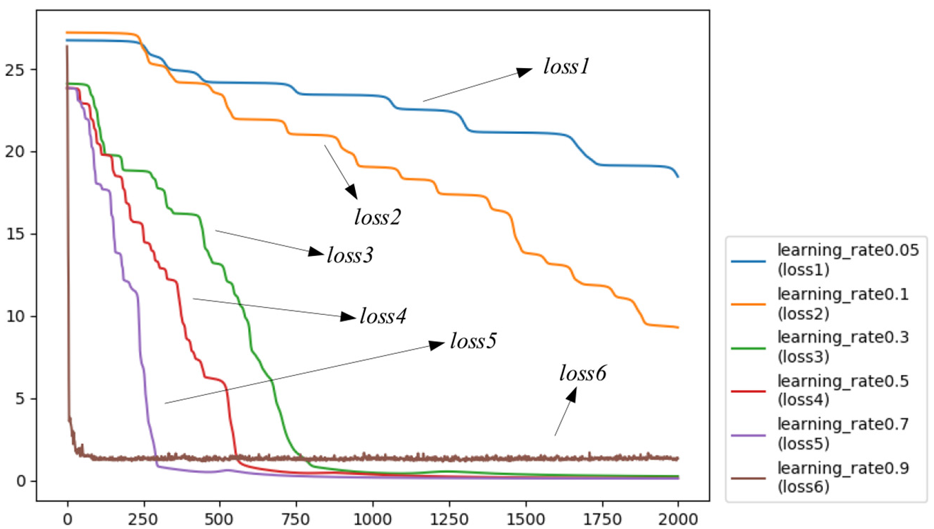
Loss with different learning rates.

Nearest neighbor threshold ε and the minimum number of MinPts

The setting of nearest neighbor threshold ε and minimum number of MinPts directly affects trajectory segments clustering results. If MinPts is set to a great value, most of trajectory segments will not meet the condition of $N_{\epsilon }(\mathrm{TS})\ge \mathrm{MinPts}$ . In most extreme cases, no trajectory segments meet such condition, which may result in all the trajectory segments being marked as noise. If MinPts is too low, the number of core trajectory segments may increase and result in too many clusters. Meanwhile, if ε is too excessive, trajectory segment that does not belong to any clusters may be clustered as a new one. While ε is too low, there will be a large number of smaller clusters, which will also lead to a large number of trajectory segments cannot be in the neighborhood, thus becoming noise. Figure 13(a)–(d) shows the influence of MinPts being too excessive, MinPts being too low, ε being too excessive, and ε being too low on clustering, respectively. The data come from a subset of synthetic trajectory data set. In order to visualize cluster results, we use t-distributed stochastic neighbor embedding (t-SNE) algorithm ³⁷ to compress multi-dimensional data into two-dimensional points. The brown dots in the graph represent noise. As can be seen from Figure 13(a), when MinPts is too excessive, a large amount of noise will be generated. Figure 13(b) and (d) shows that too small MinPts or ε can cause noise and too many clusters. Figure 13(c) shows that too excessive ε can make two different clusters be wrongly divided into one cluster. Therefore, it is important to choose the nearest neighbor threshold ε and the minimum number of MinPts.

Figure 13.

Effects of MinPts and ε on clustering results: (a) clustering with excessive MinPts (MinPts = 30), (b) low MinPts (MinPts = 2), (c) excessive ε (ε = 0.99), and (d) low ε (ε = 0.3).

Similarity index threshold ρ

In the process of anomaly detection, the similarity index obeys normal distribution. At the same time, it can avoid the deviation of detection result caused by the inaccurate threshold value ρ of similarity index. The threshold value of similarity index is determined by kσ criterion. It is more reasonable when k is 1.645. ³⁸ Figure 14 shows the distribution of the similarity index ano. The abscissa represents the value of the similarity index ano after Z-score standardization, and the ordinate represents the probability corresponding to each ano. The curve is generated after fitting the data.

Figure 14.

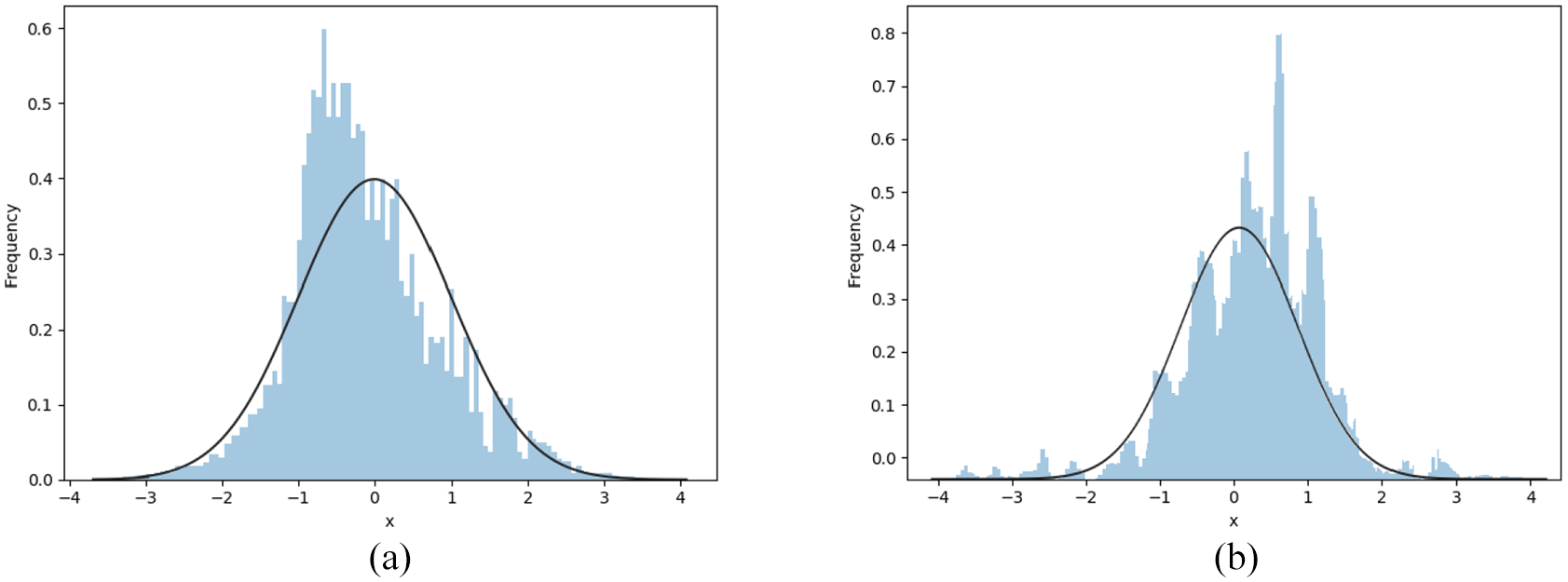
Distribution of ano: (a) North Atlantic hurricanes and (b) synthetic trajectories.

In order to conform the actual situation, the threshold value ρ only takes the boundary value on the left side, and the y( $\mathrm{an}{o}_i$ ) as shown in equation (12) can be obtained, where 0 means anomaly and 1 means normal, that is, ρ =  ${\mu }_{\mathrm{ano}}-k{\sigma }_{\mathrm{ano}}$

$$y\left(\mathrm{an}{o}_i\right)=\{\begin{array}{c}0,\mathrm{an}{o}_i\le {\mu }_{\mathrm{ano}}-k{\sigma }_{\mathrm{ano}}\hfill \\ \multicolumn{1}{c}{1,\mathrm{else}}\end{array}$$

(12)

Experimental results analysis

Synthetic trajectories

In this article, labeled artificial trajectory data set is used first to verify the unsupervised trajectory anomaly detection algorithm based on deep representation; then, we compare the detected anomaly with the label in the data set. The validity and feasibility of the algorithm are proved by high accuracy.

Figure 15 shows the loss function, with orange (light) representing the mixed feature sequence FM and blue (dark) representing the deep feature sequence FD. The learning rate sets to 0.5. After iteration, the loss of FM is gradually stable at 0.0396 and that of FD is gradually stable at 0.0389. The loss function is given by equation (5) in section “Auto-encoder.” It can be seen from the figure that the loss of FM and FD starts to decrease slowly when iterating 2000 times and 1000 times, respectively. Compared with FM, the convergence speed of FD is faster. This is because FM contains more features, so it needs more iterations.

Figure 15.

Loss function on synthetic trajectory data.

With iterating experiments for many times, we can get the parameters range or setting strategy. the minimum number threshold value MinPts is in the range of 15–25, and the nearest neighbor threshold value ε is in the range of 0.6–0.9. By calculating the cosine similarity between the mixed feature sequences representing the trajectory segments and arranging them in numerical ascending order, the nearest neighbor threshold ε can be selected. The k-distance scatter diagram shown in Figure 16 is drawn, so as to select the appropriate nearest neighbor threshold ε. In the graph, the abscissa corresponds to the sequence number of each pair of mixed feature sequences cosine similarity, and the ordinate is the value of cosine similarity. In order to facilitate observation and value taking, two different ranges are selected based on the ordinate to draw Figure 16(a) and (b). It can be seen from Figure 16(a) that the vertical coordinate of k-distance scatter diagram changes rapidly between 0.2 and 0.6, which makes the change trend front part of the scatter diagram unobservable. The k-distance scatter diagram shown in Figure 16(b) is drawn by removing the head points with cosine distance less than 0.6 and a small number of tail points with cosine distance greater than 0.9. It can be clearly seen that the cosine distance increases smoothly in the range of 0.6–0.9, and the cosine similarity between most of the mixed feature sequences is in this region. Therefore, the nearest neighbor threshold ε is more appropriate in the range of 0.6–0.9.

Figure 16.

The selection of ε: (a) k-nn (0 < cosine distance < 1) and (b) k-nn (0.6 < cosine distance < 0.9).

In order to verify the effectiveness of our algorithm and facilitate the observation of clustering effect, it is necessary to visualize the data after clustering. Similar to Figure 13, we also use t-SNE algorithm ³⁷ to compress multi-dimensional data into two-dimensional data to visualize cluster results. t-SNE is especially suitable for the visualization of high-dimensional data. Figure 17 shows the effect of clustering. Figure 17(a) shows the clustering effect of FD and Figure 17(b) shows the clustering effect of FM. It can be seen that the clustering of FM is very clear to divide the trajectory segments into five clusters, which is consistent with the label in the data set, and the effect is better than that of FD. At the same time, it can be seen from the figure that clustering with FM makes objects with similar characteristics more closely connected. Therefore, FM can be a good representation of trajectory segments and comprehensively describe the shallow and deep features of trajectory segments.

Figure 17.

Clustering results on both models: (a) FD clustering and (b) FM clustering.

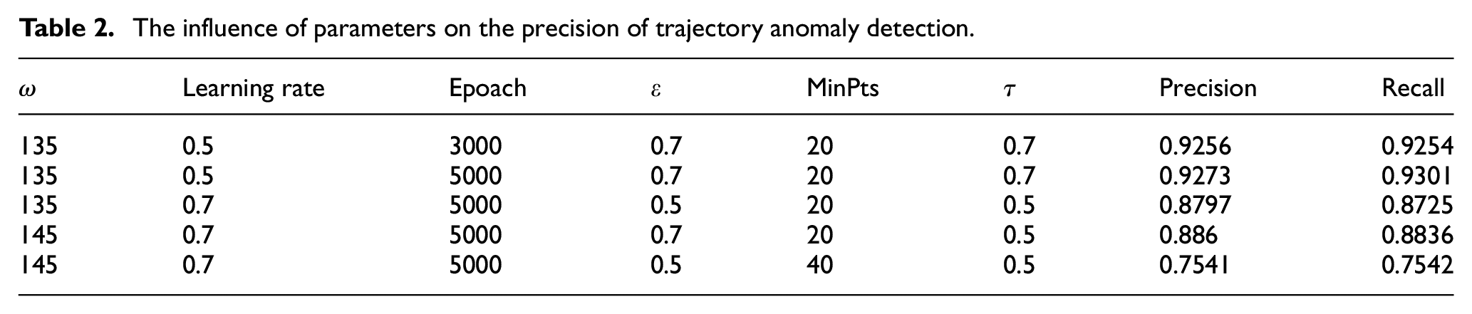
There are many parameters in TAD-FM. The setting of different parameters may affect precision and recall of anomaly detection. In this article, many groups of parameters are selected to carry out multiple experiments, and the experimental results are averaged to analyze the causes of different results caused by parameter setting. The evaluation criterion used in the experiments are precision and recall. Precision refers to the proportion of positive cases in the samples identified as positive cases. Recall represents the proportion of positive cases in the sample to be correctly predicted. The two criterion are given as equations (13) and (14)

$$\mathrm{Precision}=\frac{\mathrm{TP}}{\mathrm{TP}+\mathrm{FP}}$$

(13)

$$\mathrm{Recall}=\frac{\mathrm{TP}}{\mathrm{TP}+\mathrm{FN}}$$

(14)

where TP represents the number of samples actually positive and classified as positive by the classifier, FP represents the number of samples actually negative but classified as positive by the classifier, FN represents the number of samples actually positive but classified as negative by the classifier.

Table 2 shows the precision rate and recall rate of anomaly detection obtained by setting different parameters for experiments. It can be seen that different parameters will have a greater impact on the results. Too excessive ω will make the number of trajectory segments redundant, which is not conducive to clustering, resulting in the decline of precision and recall rate. In the case of setting the same learning rate and different iterations, the difference between the precision rate and the recall rate is not significant, because after several iterations, the difference between the two loss is very small. Too low ε and too excessive MinPts directly lead to the increase in noise during clustering, which makes the result of anomaly detection inaccurate. When τ is too low, it will affect the judgment of whether the overall trajectory is anomaly, so the precision and recall rate are low.

Table 2.

The influence of parameters on the precision of trajectory anomaly detection.

ω	Learning rate	Epoach	ε	MinPts	τ	Precision	Recall
135	0.5	3000	0.7	20	0.7	0.9256	0.9254
135	0.5	5000	0.7	20	0.7	0.9273	0.9301
135	0.7	5000	0.5	20	0.5	0.8797	0.8725
145	0.7	5000	0.7	20	0.5	0.886	0.8836
145	0.7	5000	0.5	40	0.5	0.7541	0.7542

In this article, K nearest neighbors (KNN), convolutional neural networks (CNN), support vector machines (SVM), trajectory anomaly detection with shallow feature sequence (TAD-F), trajectory anomaly detection with deep feature sequence (TAD-FD), and trajectory anomaly detection with mixed feature sequence (TAD-FM) are tested in several subsets of the data set. After many experiments, the precision of KNN is 83.96%, CNN is 87.50%, SVM is 91.29%, TAD-F is 85.46%, TAD-FD is 89.31%, and TAD-FM is 92.67%. TAD-F represents the algorithm using shallow feature sequence F, TAD-FD represents the algorithm using deep feature sequence FD, TAD-FM represents the algorithm using mixed feature sequence FM, that is, the unsupervised trajectory anomaly detection algorithm based on deep representation proposed in this article. KNN anomaly detection algorithm is a relatively simple detection method. By arranging the k-nearest neighbor distance of each object in descending order, the first n objects can be identified as outliers. The anomaly detection method using CNN is to divide the data into training set and test set and measure the effect of anomaly detection by test set. SVM is one of the most robust and accurate two classification algorithms in data mining algorithm. The idea of using SVM for anomaly detection is to divide the objects to be detected into two categories through hyperplane, namely, normal and abnormal. Figure 18 shows the precision rate of anomaly detection. It can be clearly seen from the figure that the precision rate of TAD-FM is higher than other methods in the experimental effect. Compared with TAD-F and TAD-FD, the precision of TAD-FM is 7.21% and 2.36% higher, respectively, which shows the superiority of the deep feature fusion model based on auto-encoder and can accurately, deeply, and comprehensively serialize the trajectory sequence. As a supervised learning, CNN has a good effect when the data volume is large, but it has some limitations when the training sample data are small. In experiments using artificial trajectory data sets, the precision is low because of the small amount of data. At the same time, in the daily trajectory data, there are few labeled data, which makes it difficult to detect the anomaly trajectory with the method of supervised learning. TAD-FM uses unsupervised method and mixed feature sequence to represent trajectories more comprehensively, which makes the measurement of similarity between trajectories more accurate, so the precision rate is higher. At the same time, the validity and feasibility of the algorithm can be verified by the labeled data set.

Figure 18.

Precision comparison of different algorithms.

North Atlantic hurricanes

The North Atlantic hurricanes is a data set without label. Due to the lack of ground truth, the evaluation indicators in the field of classical machine learning cannot be applied to the evaluation of anomaly detection results. Therefore, the purpose of using the North Atlantic hurricanes data set is to verify that TAD-FM can detect anomaly trajectories in the real unlabeled situation.

Figure 19 shows the loss function of experiment, the orange (light) curve represents the mixed feature sequence FM, and the blue (dark) curve represents the deep feature sequence FD. The learning rate sets 0.5. The loss of FM is gradually stable at 0.06608 and that of FD is gradually stable at 0.06244. It can be roughly seen from the figure that the loss of FM and FD does not decrease rapidly when iterating for 100 times and 700 times, respectively, and gradually decreases slowly.

Figure 19.

North Atlantic hurricane trajectories data loss function.

Figure 20 shows the clustering effect (ε: 0.7, MinPts: 25). In order to make the clustering of multi-dimensional data easy to observe, t-SNE algorithm is also used for dimension reduction. It can be seen from the clustering effect that the trajectory segments of DBSCAN algorithm are divided into six categories. Different from the simple method of dividing trajectory segments based on density alone, this article uses the mixed feature sequence to represent the trajectory segments of hurricanes. According to different feature sequence patterns, the trajectory segments are divided into different types, and anomalies are found in the same motion mode, which make the results more practical.

Figure 20.

North Atlantic hurricane trajectories data clustering.

In order to verify the effectiveness of DBSCAN in this algorithm, a variety of clustering algorithms are used to compare with DBSCAN. Figure 21 shows the silhouette coefficient of K-means, Gaussian mixture model (GMM), and birch clustering algorithms with the number of clusters between 3 and 9. The performance of clustering is evaluated by silhouette coefficient. It can be seen from the figure that when the number of clusters is 6, the contour coefficient of GMM is 0.635, which is higher than other algorithms. The silhouette coefficient of DBSCAN is 0.633, which is similar to GMM. At the same time, DBSCAN does not need to specify the number of clusters, while the other three algorithms need to determine the number of clusters in advance. Considering the practical data, DBSCAN is more practical.

Figure 21.

Comparison of silhouette coefficient.

Table 3 shows the influence of parameters on the number of anomaly trajectories. It can be seen from the table that the setting of different parameters has a significant impact on the results of anomaly detection. It is necessary to select appropriate parameters in the experiment. Too low ω will make the division of trajectory segments more detailed, but too much detail will make the number of trajectory segments too redundant, which is not conducive to the analysis of anomaly trajectories. ε and MinPts directly affect the clustering effect. If MinPts is too excessive, there will be too few core sequences and too many sequences in the same cluster. At the same time, a large number of sequences that do not belong to any cluster will become noise. On the contrary, if MinPts is too low, it will produce too many core sequences, which will increase the number of clusters. Similarly, the setting of ε will also affect the clustering results. τ considers the integrity of trajectory anomaly detection, and too excessive or too low will directly affect the number of anomaly trajectory. After many experiments, the range of nearest neighbor threshold ε is 0.6–0.9, and the minimum number threshold MinPts is 15–25.

Table 3.

The influence of parameters on the number of anomaly trajectories.

Ω	ε	MinPts	τ	Numano
125	0.6	20	0.5	63
135	0.7	25	0.5	52
135	0.6	20	0.7	41
135	0.7	25	0.7	39

In this article, TRAOD algorithm, TAD-FM algorithm, TAD-FD algorithm, and TAD-F algorithm are used for comparison. Due to the difference of anomaly detection methods, parameter settings, and calculation volume, they are not comparable in performance. Therefore, this article compares the experimental results. Figure 22(a) shows the experimental effect of TAD-FM algorithm. Figure 22(b) shows the experimental effect of TRAOD algorithm (D: 85.0, P: 0.95, F: 0.2). Figure 22(c) shows the experimental effect of TAD-F algorithm. Figure 22(d) shows the experimental effect of TAD-FD algorithm. The red line is the detected anomaly trajectory. It can be seen from Figure 22 that both algorithms can detect anomaly trajectory that are significantly different from other normal trajectory, but the detection results are different. This is because the trajectory algorithm focuses on judging the anomaly from the shape of the trajectory, while the TAD-FM algorithm transforms the spatial shape of the trajectory into the feature sequence represented by the deep fusion and judges whether the trajectory is anomaly by the cosine similarity of the feature sequence. The result of TAD-F algorithm is very messy, because only using subjective characteristics, it cannot be well integrated into the algorithm. There is a certain gap between the results of TAD-FD algorithm and TAD-FM algorithm, but it is better than TAD-F algorithm. This is because there is no comprehensive fusion of all kinds of features, which cannot detect the anomaly comprehensively. Similar trajectories in shape may have different motion modes. Similarly, trajectories with different shapes may have similar characteristics. Therefore, TAD-FM algorithm can not only find the shape of the trajectory anomalies but also find the anomalies according to the hidden features, mining the anomaly trajectory in many ways, which shows the effectiveness and feasibility of the algorithm. At the same time, in the real data set, TAD-FM algorithm can also detect the anomaly trajectory, which has good practical application value.

Figure 22.

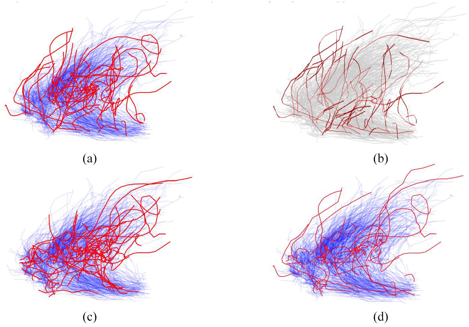
View of trajectory anomaly detection results: (a) TAD-FM, (b) TRAOD, (c) TAD-F, and (d) TAD-FD.

Some real application scenarios

Trajectory anomaly detection can be widely used in numerous spatial-temporal application scenarios such as climate monitor, animal habit analysis, and traffic detection. In this section, we introduce some typical application scenarios to intuitively describe the meaning of studying trajectory anomaly detection and point out future application directions.

1. Abnormal climate detection is one of the typical application scenarios. There are mainly two ways to find abnormal climate. One is finding outlier trajectories of various storms, typhoon as well as other meteorological data. ⁵ The other is finding the trends or periods of extreme climate using spatial and temporal weighted regression. ³⁹ Lee et al. ⁵ developed a trajectory outlier detection algorithm TRAOD. Their algorithm consists of two phases: partitioning and detection. The first phase is to partition a trajectory into a set of line segments, which ensures both high quality and high efficiency. In the second phase, they present a hybrid of the distance-based and density-based approaches. While Fotheringham et al. ³⁹ present a novel model called geographical and temporal weighted regression (GTWR) to account for local effects in both space and time dimensions. In their work, they first detailed both the model formulation and the estimation of GTWR focusing on spatiotemporal kernel function definition and spatiotemporal band width optimization. Then, the performance of GTWR was examined by comparison with basic geographical weighted regression models.

2. Animal habit analysis is a very important application of trajectory analysis. Li et al. ⁴⁰ developed an efficient prototype system called MoveMine to discover animal movement patterns from animal movement data. Animal abnormal habits or moving tendencies may be events or observations that do not conform to an expected pattern. These finds can greatly attract the attention from biologists or even botanists.

3. Urban traffic detection is very important for city life. Both spatial and temporal outliers can be detected from traffic data. Through analyzing trajectories in urban area or with constraint of road network, different traffic flow can be identified. Urban traffic detection is very helpful for smart city plan and smart transportation management. Li et al. ⁴¹ proposed a temporal outlier discovery framework for detecting temporal outliers from vehicle traffic data. In their work, agglomerated temporal information of the entire data set is utilized to detect outliers. At each time stamp, similarity of each road segment is checked with other road segments, and historical similarities of each road segment are recorded in a temporal neighborhood vector. Finally, outliers are detected from drastic changes.

4. Urban safety management has been considered as a new important application of trajectory moving mining. The movement of crowds in a city is strategically important for risk assessment and public safety management. ² Therefore, through analyzing the status of traffic flow and communication base stations, the direction and density of moving crowds can be extracted, and quick response to the urban safety management can be provided to the city administrator. In the work of Hoang et al., ⁴² a practical solution for citywide traffic prediction was developed. First, they partition the map of a city into regions using both road network and human historical mobility records. In order to model multiple complex factors that affect crowd flows, they decompose flows into three components: seasonal patterns, trend, and residual flows. Their method is scalable and outperforms compared with some baselines.

Conclusion

Some current trajectory anomaly detection algorithms cannot fully take the characteristics of trajectories into account, and they are also limited by the space attribute of trajectories. In order to solve these problems, we propose an unsupervised trajectory anomaly detection algorithm based on deep representation (TAD-FM) in this article. Attributes of trajectories are deeply studied and their shallow features are extracted. Meanwhile, a deep feature fusion model based on the auto-encoder is present to obtain the mixed features of trajectories expressed by fusing both shallow and deep features. This model can comprehensively consider features of trajectories themselves. The feature sequence is used to represent trajectories and their anomalies, through which, the limitation of spatial attribute can be reduced. The experimental results show that TAD-FM algorithm has higher accuracy and can find the inconspicuous anomaly trajectories and their segments comprehensively.

As discussed above, trajectory anomaly detection is quite important for many fields. Most trajectory data are label free, and traditional classification algorithms cannot work on such data directly. Therefore, how to find anomaly using state-of-art machine learning algorithms is a challenge. Moreover, without ground-truth data, how to assess the results is another challenge.