Sage Journals: Discover world-class research

Abstract

The traditional dynamic balance methods require multiple start-stop operations for test weight adjustments, leading to high resource consumption. To improve the efficiency, accuracy, and safety of aero-engine rotor dynamic balancing, a novel dynamic balancing optimization method is proposed. A virtual prototype model of the high-speed aero-engine rotor is constructed to analyze its dynamic characteristics and derive the transfer function under unbalanced excitation. Subsequently, equilibrium equations are established to relate the unbalanced response to rotor amplitude. A multi-strategy improved sparrow search algorithm is then applied. The optimization minimizes the sum of squared residual vibrations and the maximum residual vibration at each measurement point. Experimental verification is conducted on a simulated test bench for a specific type of turbine rotor used in aerospace engines. The results demonstrate that the proposed method improves test weight efficiency and prevents local vibration overruns. It achieves an average vibration reduction of 52.56%, outperforming the 45.23% of traditional on-site dynamic balancing. This approach offers a valuable technical reference for aerospace engine vibration control.

Keywords

rotor of high-speed aero-engine balance without trial weights sparrow search algorithm dynamic balance optimization virtual prototype

Introduction

The high-performance flexible rotor serves as the core component of the aero-engine, featuring a complex structure and operating in a demanding environment. It is required to endure extreme conditions of high temperature, pressure, and rotational speed, with its reliability directly influencing engine safety.^1–3 In recent years, the pursuit of a higher thrust-weight ratio has driven the adoption of lightweight designs for aero-engine components.^4,5 However, due to their slender and often hollow design under high-speed rotation conditions, flexible rotors are highly sensitive to even minor imbalances. This sensitivity can lead to deformation and disrupt equilibrium, resulting in complex vibration issues.⁶ Statistics indicate that rotor imbalance is the leading cause of vibration-related failures, accounting for more than half of all engine faults. When operating at high speeds, rotors may exceed second or third-order critical speeds, further complicating vibration control. As a result, achieving dynamic balance in high-speed rotors has become a fundamental requirement in aero-engine design and manufacturing.⁷

The conventional approach to balancing high-speed rotors relies on the influence coefficient and modal balance methods.⁸ The influence coefficient method is widely used in practical applications due to its simplicity and effectiveness. It establishes a mathematical model that links correction mass to rotor vibration, enabling efficient calculation of the unbalanced vector through a vector feedback mechanism.⁹ The modal balance method, in contrast, aims to reduce vibrations across the entire speed range. By decomposing vibrations into different modes based on unbalanced vibration and vibration mode, it effectively suppresses unbalanced responses.¹⁰ Although dynamic balancing methods based on these principles effectively suppress vibrations, their implementation often requires multiple trial weights to determine the unbalanced vector. This process demands highly skilled technicians to ensure accuracy. Improper selection of test weights may cause excessive vibrations during balancing, potentially damaging the rotor and increasing operational risks. To address these challenges, it is essential to develop a trial weight-free dynamic balancing method.¹¹ By reducing or eliminating trial weight steps and directly obtaining the imbalance distribution of rotor, this approach enhances safety, efficiency, and reliability in dynamic balancing operations.

In recent years, the methods of dynamic balance of rotor without trial weight have evolved into three main categories: virtual simulation dynamic balance technology, influence coefficient backstepping correction method, and intelligent optimization dynamic balance method. Among these methods, virtual simulation dynamic balancing technology replaces physical testing with rotor dynamics modeling, providing feedback on the rotor’s overall operating state without requiring trial weights for imbalance correction. Khulief et al.¹² utilized modal information to identify rotor imbalance and performed dynamic balancing on a selected correction plane. Based on instantaneous mode analysis, Zhao et al.¹³ established a relationship between unbalance and transient excitation force to identify rotor system unbalance. Sanches et al.¹⁴ applied augmented Kalman filter technology to balance flexible rotors without trial weights and proposed a data-driven experimental approach to validate its effectiveness. The influence coefficient backstepping correction method determines the influence coefficient through empirical formulas or prior measurements, establishing a correlation between rotor unbalance and vibration. Xie et al.¹⁵ determined the magnitude of the influence coefficient using an empirical formula, determined the lag angle based on the generator set’s lag phase. By combining these factors, they estimated both the size and phase of unbalance. Ranjan and Tiwari¹⁶ proposed an enhanced influence coefficient method that improves balancing efficiency by using high-speed influence coefficients along with low-speed identified unbalances. Ye et al.¹⁷ derived similarity relations and influence coefficients for rotor systems based on dynamic similarity theory, enabling a trial weight-free dynamic balance experiment by applying these similarity relations. The intelligent optimization dynamic balancing method utilizes machine learning algorithms to establish the correlation between rotor unbalance and vibration, enabling trial weight-free dynamic balancing. Yao et al.¹⁸ proposed a multi-speed dynamic balancing method for flexible rotors based on a genetic algorithm combined with a bi-objective optimization approach. Zhong et al.¹⁹ applied unsupervised deep learning techniques to predict imbalance amplitude and phase by analyzing collected system data, which is then used to calculate the required correction mass. Garpelli et al.²⁰ leveraged simulation data from finite element modeling and hydrodynamic bearings governed by the Reynolds equation, utilizing a standard artificial neural network for node position localization and a physically guided neural network for quantifying imbalance amplitude and phase angle.

To enhance the efficiency and precision of rotor dynamic balancing, this paper proposes a novel optimization method for high-speed aero-engine rotors without trial weights by integrating the three aforementioned approaches. The method utilizes a virtual prototype model of high-speed aero-engine rotors to determine the transfer function and employs the Whale-Cauchy-Sparrow Search Algorithm (WCSSA) to compute the correction mass, minimizing residual vibrations at each speed. The structure of this paper is as follows: Section “Dynamic balancing optimization method” introduces the proposed dynamic balancing method for high-speed aero-engine rotors without trial weights, based on the WCSSA approach. Section “Example of dynamic balance” analyzes a case study of dynamic balancing in high-speed aero-engine rotors. Section “Experimental verifications” conducts the method through experimental verification, while Section “Conclusion” offers concluding remarks and future research prospects.

Dynamic balancing optimization method

The principle of dynamic balance

Rotor unbalance refers to the phenomenon that the center of mass does not coincide with the rotation axis due to the uneven mass distribution of the rotor in the rotating machinery. When there is an unbalance in any flexible rotor system, the trajectory of the center of mass along the rotor axis presents a complex three-dimensional spatial distribution, as shown in Figure 1.

Figure 1.

Distribution diagram of rotor unbalance.

If a thin disk is taken at any section of the rotor, the centrifugal force generated by the eccentricity of the thin disk can be expressed as:

d F = e (z) d m (z) w^{2} = u (z) d z w^{2}

(1)

where dF is the centrifugal force generated by the eccentricity of the thin disk, dz is the thickness of the thin disk, e(z) is the offset of the center of mass, dm(z) is the unbalanced mass, and w is the rotor speed.

The centrifugal force is decomposed into dF_x, which is parallel to the axis in the horizontal direction, and dF_y, which is opposite to the axis in the vertical direction. This decomposition can be expressed as:

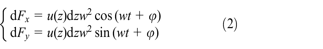
{\begin{matrix} d F_{x} = u (z) d z w^{2} \cos (wt + φ) \\ d F_{y} = u (z) d z w^{2} \sin (wt + φ) \end{matrix}

(2)

where u(z) = e(z)dm(z) is the distribution function of unbalance, and $φ$ is the phase of unbalance.

The vibration results from the time-varying magnitude and direction of the unbalanced force. The frequency of this unbalanced vibration is directly related to the rotational speed. By integrating the centrifugal force across the entire rotor, an expression for the total centrifugal force can be derived as follow:

F = w^{2} \int_{0}^{h} u (z) d z

(3)

where h is the length of the shaft.

The core of rotor dynamic balancing is addressing the issue of centrifugal force induced by an imbalanced mass. This challenge is effectively addressed using the transfer function approach.²¹ The goal of this technique is to develop an accurate dynamic model that enhances the understanding of the system’s behavior, particularly by establishing the relationship between the excitation caused by the imbalanced mass and rotor vibration response. By employing this model in conjunction with deterministic correlations that link transfer function matrices to influence coefficient methods, it becomes possible to precisely identify both the locations and magnitudes of any unbalance in the system, eliminating the need for actual trial operations.

According to the relevant principles of the dynamic model,^22,23 when an imbalance occurs in the rotor, the dynamic differential equation governing the rotor system can be formulated as follows:

M \overset{\cdot\cdot}{θ} (t) + C \overset{\cdot}{θ} (t) + K θ (t) = U Ω^{2} e^{j Ω t}

(4)

where $\overset{\cdot\cdot}{θ} (t)$ , $\overset{\cdot}{θ} (t)$ , and $θ (t)$ are the acceleration, velocity, and displacement of the rotor offset equilibrium position, respectively M , C , and K are the mass, damping, and stiffness matrices of the shaft, respectively. U is the unbalanced excitation matric, and $Ω$ is the angular frequency.

Assuming that the particular solution of the unbalanced response of equation (4) is $θ (t) = A e^{j Ω t}$ , then equation (4) can be solved as follows:

A = Ω^{2} H (Ω) U

(5)

where $H (Ω)$ is the transfer function matrix of the rotor system, which is expressed as $(K - Ω^{2} M + j Ω C)^{- 1}$ ; A is the complex matrix to be determined, which represents the amplitude and phase of the response.

The influence coefficient method can be expressed as:

T (Ω) Q + V = R

(6)

where, $T (Ω)$ is the influence coefficient, Q is the correction mass, V is the vibration measured at the measurement section, and R is the residual vibration.

When considering rotor balance at K speeds using the influence coefficient method, the system can be organized into an M × K row and N column matrix, where M represents the number of measurement points and N denotes the number of balance surfaces. The influence coefficient method is mathematically represented as²⁴:

\begin{matrix} [\begin{matrix} T_{11}^{1} & T_{12}^{1} & \dots & T_{1 N}^{1} \\ T_{21}^{1} & T_{22}^{1} & \dots & T_{2 N}^{1} \\ ⋮ & ⋮ & ⋱ & ⋮ \\ T_{J 1}^{1} & T_{J 2}^{1} & \dots & T_{JN}^{1} \\ T_{11}^{2} & T_{12}^{2} & \dots & T_{1 N}^{2} \\ T_{21}^{2} & T_{22}^{2} & \dots & T_{2 N}^{2} \\ ⋮ & ⋮ & ⋱ & ⋮ \\ T_{M 1}^{n} & T_{M 2}^{n} & \dots & T_{MN}^{n} \\ ⋮ & ⋮ & ⋱ & ⋮ \\ T_{M 1}^{K} & T_{M 2}^{K} & \dots & T_{MN}^{K} \end{matrix}] [\begin{matrix} Q_{1}^{1} \\ Q_{2}^{1} \\ ⋮ \\ ⋮ \\ Q_{l}^{n} \\ ⋮ \\ ⋮ \\ ⋮ \\ ⋮ \\ ⋮ \\ Q_{N}^{K} \end{matrix}] + [\begin{matrix} V_{1}^{1} \\ V_{2}^{1} \\ ⋮ \\ ⋮ \\ V_{l}^{n} \\ ⋮ \\ ⋮ \\ ⋮ \\ ⋮ \\ ⋮ \\ V_{M}^{K} \end{matrix}] = [\begin{matrix} R_{1}^{1} \\ R_{2}^{1} \\ ⋮ \\ ⋮ \\ R_{l}^{n} \\ ⋮ \\ ⋮ \\ ⋮ \\ ⋮ \\ ⋮ \\ R_{M}^{K} \end{matrix}] \end{matrix}

(7)

where $T_{MN}^{K}$ is the influence coefficient of the Nth correction surface on the Mth vibration measurement section at the Kth rotational speed, $Q_{N}^{K}$ is the correction mass applied by the Nth correction surface at the Kth rotational speed, $V_{M}^{K}$ is the vibration of the Mth vibration measurement section at the Kth rotational speed, and $R_{M}^{K}$ is the residual vibration of the Mth vibration measurement section at the Kth rotational speed.

Assuming that the residual vibration R = 0 corresponds to complete balance, the relationship between the transfer function matrix and the influence coefficient can be derived by comparing equations (5) and (6), and is expressed as:

T (Ω) = Ω^{2} H (Ω)

(8)

The relationship between the transfer function matrix and the influence coefficient method is obtained. For the solution of the influence coefficient method, when M × K = N, the number of equations matches the number of equilibrium planes. In this case, with the residual vibration R = 0, the influence coefficient method has a unique solution, which can be expressed as:

Q = - T (Ω)^{- 1} V

(9)

When M × K > N, that is, the number of equations is greater than the number of equilibrium planes, equation (7) is a contradictory equation set, and the least square method is usually used to minimize the sum of residual vibration squares of each measurement point. According to the minimum condition of residual vibration R, the correction weight of each balance plane can be solved as:

Q = - (T (Ω)^{* T} T (Ω))^{- 1} T (Ω)^{* T} V

(10)

where $T (Ω)^{* T}$ is denoted by $T (Ω)$ conjugate transpose matrix.

Although the least square method can minimize the square sum of residual vibrations when solving the overdetermined equation problem, it may cause some counterweights to exceed the acceptable limit of the equilibrium plane correction, resulting in significant residual vibrations at some measurement points. To overcome these limitations, a WCSSA-based solution method is proposed. By optimizing the minimum sum of squared residual vibrations using WCSSA, an optimal balance weight is obtained to minimize the total residual vibration across all measurement points. Additionally, by setting the minimization of the maximum residual vibration at each measurement point as the optimization objective and utilizing an enumeration method to solve for the corrected balance amounts after convergence, a counterweight scheme is established with minimal maximum residual vibration at each measurement point.

WCSSA optimization algorithm

The Sparrow Search Algorithm (SSA) is an optimization algorithm inspired by the foraging behavior of natural sparrow groups. Initially proposed by Xue and Shen²⁵ in 2020, SSA aims to achieve global optimal solutions through collaborative group efforts and information exchange. With its intuitive model based on biological principles, concise implementation logic, and dynamic balance between exploration and exploitation strategies, SSA demonstrates significant potential for diverse applications, versatility, and adaptability. However, the algorithm faces challenges, including performance fluctuations due to parameter sensitivity, susceptibility to local optima traps in complex scenarios, and instability stemming from random initialization results. To address these issues, this study proposes the following improvements to enhance the SSA algorithm:

(1) The Iterative Chaotic Map with Infinite Collapses (ICMIC) is introduced to replace the initial population function, thereby augmenting the randomness and diversity of particles in the optimization process. Unlike the original approach, this method offers several advantages, including more uniform traversal of the search space and faster convergence.²⁶ The mathematical expression for this approach is given as follows:

x_{i + 1} = \sin (\frac{a}{x_{i}})

(11)

where a represents the control parameter, x_i represents the variable value at i iterations, and x_i₊₁ represents the variable value at i +1 iteration.

(2) In the initial stage, the global exploration strategy of the Whale Optimization Algorithm (WOA)²⁷ is employed to replace the position update mechanism of the discoverer in the original sparrow algorithm. This substitution effectively addresses the excessive reliance of the sparrow algorithm on position updates from previous generations, enhancing its ability to explore the solution space more broadly. The corresponding formula can be expressed as follows:

X_{i}^{d} (t + 1) = {\begin{matrix} X_{g}^{d} (t) - A \times D \times | X_{i}^{d} (t) - X_{g}^{d} (t) |, p \\ X_{i}^{d} (t) + A \times D \times | X_{r}^{d} (t) - X_{i}^{d} (t) |, (1 - p) \end{matrix}

(12)

where $X_{i}^{d} (t + 1)$ denotes the updated value of the position of ith sparrow on the dth dimension at the t + 1 generation; $X_{g}^{d} (t)$ represents the value of the current global optimal position in the d-dimension; $X_{i}^{d} (t)$ represents the value of the current position of ith sparrow on the dth dimension at the tth generation; $X_{r}^{d} (t)$ represents the position of a sparrow randomly selected in the t-th generation in the d-th dimension; A is a control parameter, defined as A = 2a × r−a, where a is a linear decreasing control parameter, decreasing from 2 to 0; r is a random vector between [0, 1]; D is a distance parameter used to determine the step size of the position update, which is defined as $D = | C \times X * (t) - X (t) |$ , where C = 2r; $X * (t)$ is the current optimal solution location.

(3) The Cauchy mutation strategy²⁸ is employed to replace the follower position update formula in the original sparrow algorithm, significantly expanding the exploration range and diversity of the algorithm. This enhancement effectively mitigates premature convergence and improves the balance between global search and local exploitation, owing to the long-tailed characteristics of Cauchy distribution. It also increases adaptability to initial value sensitivity and environmental variations of the algorithm. Particularly, when addressing multimodal and non-convex optimization problems, the inclusion of the Cauchy distribution facilitates exploration across diverse solution regions. Consequently, while preserving algorithmic simplicity, this modification significantly boosts its solution capability and robustness in complex scenarios. The corresponding formula can be expressed as:

x_{i, j}^{t + 1} = x_{i, j}^{t} + γ \times Cauchy (0, 1)

(13)

f (x) = \frac{1}{π (1 + x^{2})}

(14)

where $γ$ is a scaling factor used to adjust the intensity of variation, $Cauchy (0, 1)$ represents the Cauchy distribution random number with a mean value of 0 and a scale parameter of 1, and f(x) is the probability density function of the Cauchy distribution.

The flow chart of the improved WCSSA algorithm is shown in Figure 2.

Figure 2.

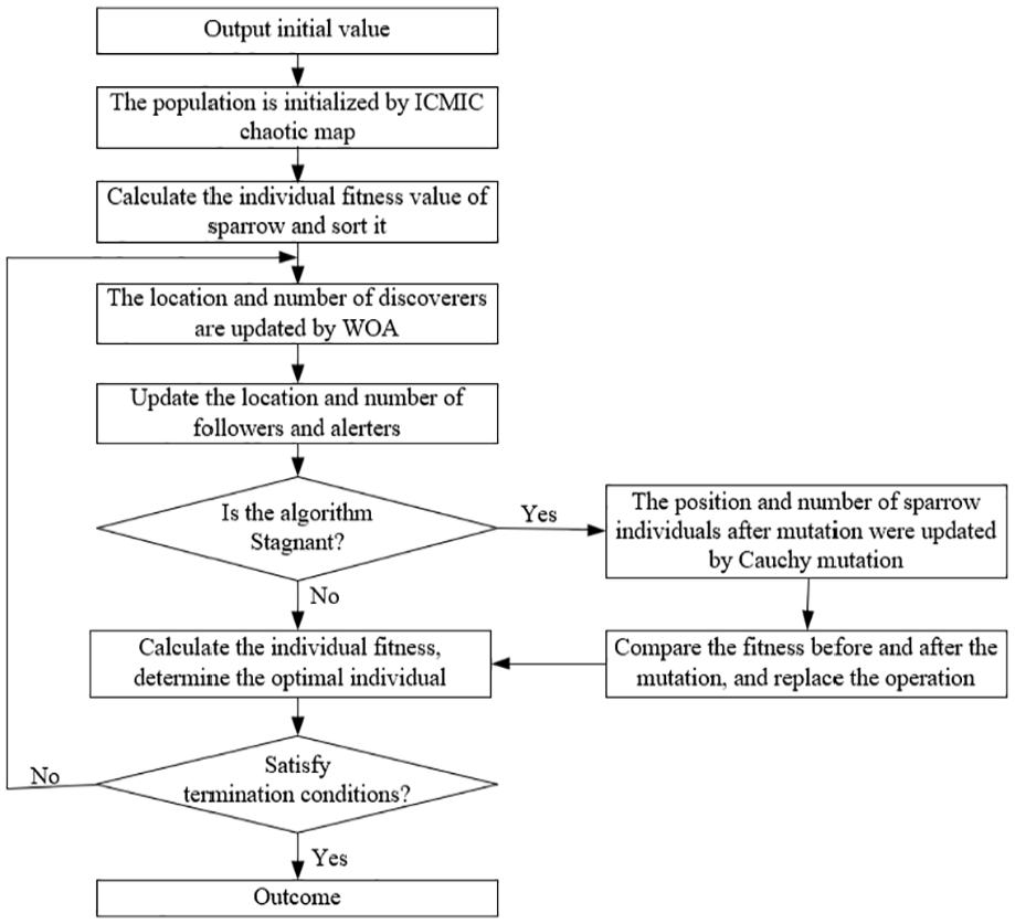
WCSSA algorithm flow chart.

WCSSA algorithm verification

To validate the advantages of the WCSSA, a comparison is conducted between the WCSSA and other optimization algorithms, including the original SSA, Subtraction-Average-Based Optimizer²⁹ (SABO), Dung Beetle Optimizer³⁰ (DBO), and Artificial Gorilla Troops Optimizer³¹ (GTO), using the CEC2021 test function.³² All parameters are kept consistent, with a population size of 100 and a maximum number of iterations set to 80. Figure 3 illustrates the optimization results for the selected test functions. It can be observed that the enhanced WCSSA outperforms the other algorithms, demonstrating superior optimization accuracy, faster convergence toward optimal solutions, and strong capabilities in both local development and global exploration.

Figure 3.

Comparison of the results of five optimization algorithms: (a) single peak function F1 test optimization results, (b) multimodal function F3 test optimization results, and (c) mixed function F9 test optimization results.

Design process of dynamic balance optimization

Following the steps of the WCSSA, a dynamic balance optimization process for high-speed aero-engine rotors is designed. First, the virtual prototype model of the high-speed aero-engine rotor is created using finite element software. To ensure the accuracy of the virtual prototype, the first two natural frequencies of the rotor system are obtained through modal analysis experiments. The support stiffness and structural damping parameters of the virtual prototype are then validated using the finite element software. Finally, the frequency deviation between the simulated modes and the measured results converges to less than 5%, thus meeting the engineering accuracy requirement of an error not exceeding 5%. The required measurement points M, speeds K, balance surfaces N, original vibration V, and transfer function $H (Ω)$ are obtained through harmonic response and modal analyses. The derived transfer function $H (Ω)$ is then substituted into equation (8) to derive the influence coefficient matrix. Next, both the original vibration V _M and influence coefficient matrix T _MN are input into WCSSA for optimization. Each sparrow represents a balance correction Q _N, which is decomposed according to equation (2), as it takes the form of a Q _N vector. Similarly, the transformed influence coefficient matrix T _MN and original vibration V _M undergo decomposition. The optimization model can be expressed as:

min (f = \sum_{i = 1}^{N \times M} ((R X_{i})^{2} + {(R Y_{i})}^{2}))

(15)

where RX = T _MN X × Q _N X + V _M X , R Y = T _MN Y × Q _N Y + V _M Y .

After calculating the weight solution set using the WCSSA, an enumeration strategy is employed for further detailed exploration. As a comprehensive solution method, the enumeration approach possesses a core advantage in completeness, ensuring that all potential solution spaces are fully traversed. This guarantees the discovery of all feasible solutions and the identification of the optimal counterweight scheme under specific optimization objectives, such as minimizing the maximum residual vibration at each measurement point. To achieve the goal of minimizing the maximum residual vibration of each measuring point, the enumeration method is applied to the counterweight solution set obtained by WCSSA. The process involves substituting candidate counterweight solutions for each balancing surface into the influence coefficient method to evaluate residual vibration levels at each measurement point under different counterweight configurations. The configuration that minimizes maximum residual vibration amplitude is then selected. The optimization model can be expressed as:

min (f_{MK} = \sqrt{R X^{2} + R Y^{2}})

(16)

where f_MK is the residual vibration of the Mth measurement point at the Kth rotational speed.

Starting from the first solution of the counterweight set and progressing to the last solution, M measurement points are identified within the solution set. The solution that minimizes the maximum residual vibration across K rotational speeds is then selected. The corresponding counterweight represents the final counterweight. By following this process, only a minimal amount of measured data is needed for rotor dynamic balancing, eliminating the traditional need for repeatedly adding or removing test weights during the balancing procedure. The overall flowchart of this process is shown in Figure 4.

Figure 4.

Overall flow chart of dynamic balance of high-speed aero-engine rotor without trial weight.

Example of dynamic balance

Virtual prototype modeling

The structural diagram of the high-speed aero-engine rotor is depicted in Figure 5. It primarily consists of a hollow slender shaft, a short shaft, and dual turbine disks, with a balancing convex platform located on the slender shaft. The dimensions are as follows: L₁ = 9.747 × 10⁻¹ m for the slender shaft, L₂ = 1.357 × 10⁻¹ m for the short shaft, D₁ = 2.4 × 10⁻¹ m for the turbine disk diameter, D₂ = 5.4 × 10⁻² m for the short shaft diameter, D₃ = 3.12 × 10⁻² m for the long shaft diameter, and D₄ = 3.7 × 10⁻² m for the balance boss diameter. The shaft material is 42CrMo steel, while the remaining structural components are made of C45E4 steel. The relevant material properties are listed in Table 1.

Figure 5.

Rotor system structure diagram.

Table 1.

Material properties.

Material	Density (kg/m³)	Young’s modulus (MPa)	Poisson ratio
42CrMo	7.85 × 10³	2.12 × 10⁵	0.28
C45E4	7.85 × 10³	2 × 10⁵	0.3

The rotor system is supported by three fulcrums: support No.1 employs an angular contact ball bearing, support No.2 utilizes a deep groove ball bearing, and support No.3 is equipped with a cylindrical roller bearing. The short and slender shafts are connected through an interference fit, transmitting torque via a spline mechanism. The first-stage turbine disk is securely fastened to the second-stage turbine disk using stop faces and end faces, fastened together with bolts. The two-stage turbine disk is suspended on the right side of support No.3.

The high-speed aero-engine rotor system is modeled in three dimensions using SolidWorks software and then imported into Ansys for virtual prototype modeling. To accurately simulate the dynamic characteristics of the rotor, the model incorporates three fundamental principles: mass, stiffness, and mode. To simplify the actual model, as shown in Figure 6, certain approximations are made while retaining key features necessary for dynamic analysis.

Figure 6.

Simulation simplified model.

The three fulcrum supports are modeled using the COMBIN214 bearing element in the analysis conducted with Ansys. As depicted in Figure 7, the relevant stiffness and damping coefficients are determined based on actual operational conditions. For support No.1, the stiffness K₁₁,₂₂ = 4.6 × 10⁸ N/m and damping C_11,22 = 20 N/(m/s) are set accordingly. Similarly, for support No.2, the stiffness K₁₁,₂₂ = 4.6 × 10⁸ N/m and damping C_11,22 = 20 N/(m/s) are assigned. Support No.3 is considered an elastic support with a stiffness of K₁₁,₁₂ = 2 × 10⁷ N/m and a damping coefficient of C₁₁,₂₂ = 1500 N/(m/s).

Figure 7.

Dynamic diagram of COMBIN214 bearing element.

After completing the configuration, the model is meshed, as mesh quality directly affects both computational efficiency and accuracy. An excessively fine mesh may increase computation time or even lead to failure. Therefore, in this study, tetrahedral elements are used for the shaft section mesh at the turbine disk and support 2, while hexahedral elements are applied to other regions. The size of each mesh element is set to be 6 × 10⁻³ m, as illustrated in Figure 8. The total number of units amounts to 234,878 with a corresponding node count of 408,255. It should be noted that unit quality reaches an impressive value of 0.85941,³³ indicating excellent grid performance.

Figure 8.

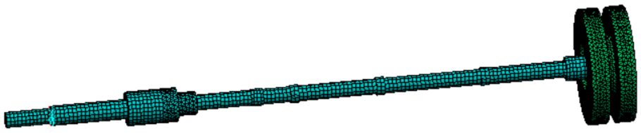
Model grid division diagram.

Dynamics analysis

The rotational speed range is set from 0 to 27,000 revolutions per minute (r/min), with the rotation occurring within the Y-Z plane, where the +Y axis phase is designated as 0° angle reference point. To account for potential spiral effects, a constraint is applied to limit the far-end axial displacement. A modal response analysis is then performed on a virtual prototype model of the aero-engine rotor system, resulting in the generation of the Campbell diagram shown in Figure 9. Given that real-world rotor systems typically demonstrate synchronous forward whirling behavior during operation, the critical speed analysis focused exclusively on this scenario. The analysis determined the first-order critical speed (W₁) to be 7365.7 r/min and second-order critical speed (W₂) to be 11,610 r/min.

Figure 9.

Campbell diagram of virtual prototype model.

To validate the accuracy of virtual prototype model, a modal test is conducted on the aero-engine rotor. The secondary turbine disk is excited, and the resulting frequency response curve in the frequency domain is presented in Figure 10. The first-order and second-order natural frequencies are identified as 123.15 and 198.79 Hz, respectively. The average error is 1.48%, and the maximum error is 2.6%, both within the commonly accepted engineering tolerance of 5%. Although there exists overall agreement between the experimentally obtained natural frequencies and those simulated using Ansys, some discrepancies may arise due to factors such as rotor damage or bending, non-uniform material properties, or assembly errors.

Figure 10.

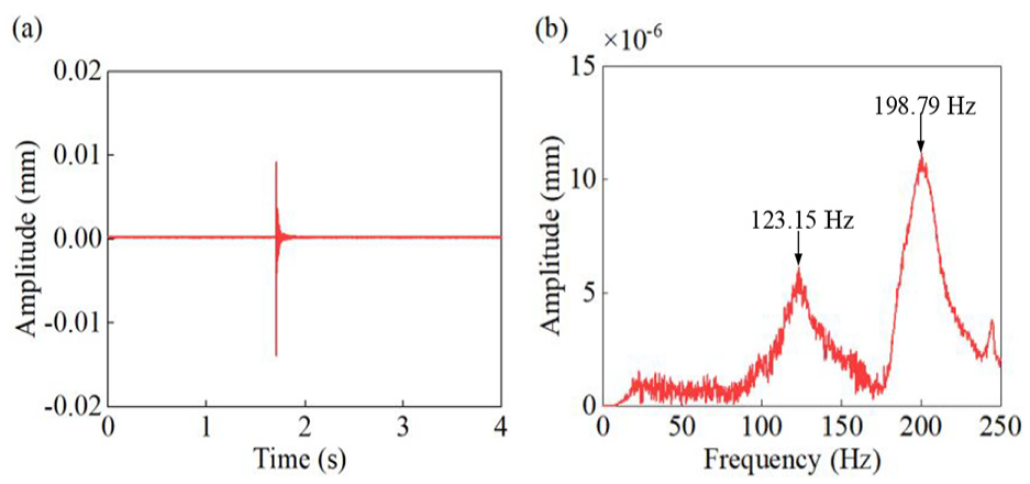
Modal test: (a) time domain signal and (b) frequency domain signal.

After conducting experimental verification on the virtual prototype model of the high-speed aero-engine rotor, an analysis of the modal shape is performed. The first-order, second-order, and third-order modes are illustrated in Figure 11. It can be observed that the first and second modes exhibit U-shaped bending near the midpoint of the shaft, while the third mode demonstrates an overall S-shaped bending of the shaft.

Figure 11.

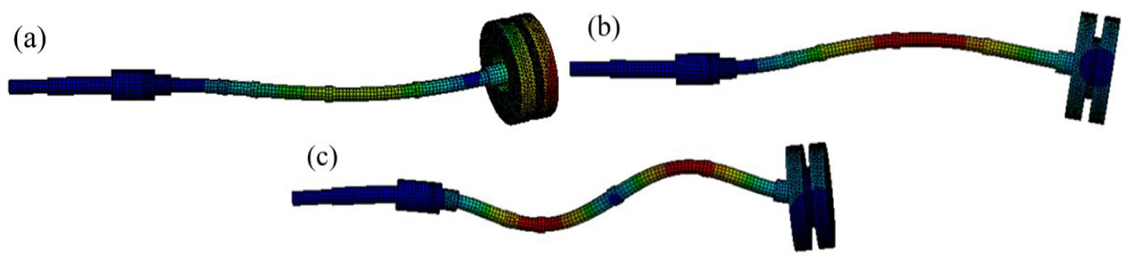
Modal shape diagram: (a) first-order modal shape, (b) second-order modal shape, and (c) third-order modal shape.

Through the analysis of vibration modes, it is evident that three measurement points can be established for dynamic balance assessment of the aero-engine rotor system, specifically at the anti-nodes of the vibration modes. Measurement points 1 is located at the middle section of the shaft near support 2, measurement point 2 is positioned at the middle section of the shaft near support 3, and measurement point 3 corresponds to the turbine disk.

Measurement points 1 is positioned in the middle section of the shaft near support NO.2, measurement point 2 is situated in the middle section of the shaft near support NO.3, and measurement point 3 corresponds to the turbine disk. Additionally, a mass point with a simulated unbalanced magnitude of 15 g, an eccentricity of 1.05 × 10⁻¹ m, and a phase shift of 180° is introduced onto the turbine disk, as illustrated in Figure 12.

Figure 12.

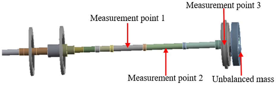
Measurement point distribution of aero-engine rotor virtual prototype.

A harmonic response analysis is performed on the virtual prototype of the high-speed aero-engine rotor, considering the second-order critical speed at 193.5 Hz. The frequency range for the analysis is set from 0 to 300 Hz. Four equilibrium surfaces are subjected to an unbalanced excitation of 15 g with a phase shift of 180°. The resulting amplitude-frequency response curve is presented in Figure 13.

Figure 13.

Frequency response curve: only the first balance surface is added with unbalanced excitation (a) amplitude-frequency diagram, (b) phase-frequency diagram ; only the unbalanced excitation (c) amplitude-frequency diagram, (d) phase-frequency diagram are added to the second equilibrium surface; only the unbalanced excitation (e) amplitude-frequency diagram, (f) phase-frequency diagram are added to the third equilibrium surface and only the unbalanced excitation (g) amplitude-frequency diagram, (h) phase-frequency diagram are added to the fourth equilibrium surface.

The amplitude-frequency diagram (a) and the phase-frequency diagram (b) in Figure 13 are exclusively based on the addition of unbalanced excitation to the first equilibrium surface. Similarly, the amplitude-frequency diagram (c) and phase-frequency diagram (d) in Figure 13 solely represent the effects of adding unbalanced excitation to the second equilibrium surface. Furthermore, Figure 13(e) and (f) depict only the amplitude-frequency and phase-frequency diagrams when unbalanced excitation is applied to the third equilibrium surface. Lastly, Figure 13(g) and (h) illustrate solely the amplitude-frequency and phase-frequency diagrams resulting from applying unbalanced excitation to the fourth equilibrium surface. The response of the four balance surface measurement points is evident in the above figure, with amplitude peaks occurring near 122 and 194 Hz when subjected to unbalanced excitation. This observation is consistent with the results from the modal analysis. Based on the simulation outcomes and in compliance with the permissible operational range for the test bench, rotor balancing is performed at speeds of 4700, 5000, 5300, and 5600 r/min.

Dynamic balance optimization method based on WCSSA

The transfer function $H (Ω)$ of the high-speed aero-engine rotor virtual prototype system is defined as:

H (Ω) = \frac{Y (Ω)}{X (Ω)}

(17)

where $Ω$ represents the angular frequency, $Y (Ω)$ represents the output vibration response, and $X (Ω)$ represents the input excitation.

The dynamic balancing method for this high-speed aero-engine rotor involves three measurement points and four balancing surfaces. Consequently, the transfer function matrix at a given speed can be expressed as

H (Ω) = [\begin{matrix} H_{11} & H_{12} & H_{13} & H_{14} \\ H_{21} & H_{22} & H_{23} & H_{24} \\ H_{31} & H_{32} & H_{33} & H_{34} \end{matrix}]

(18)

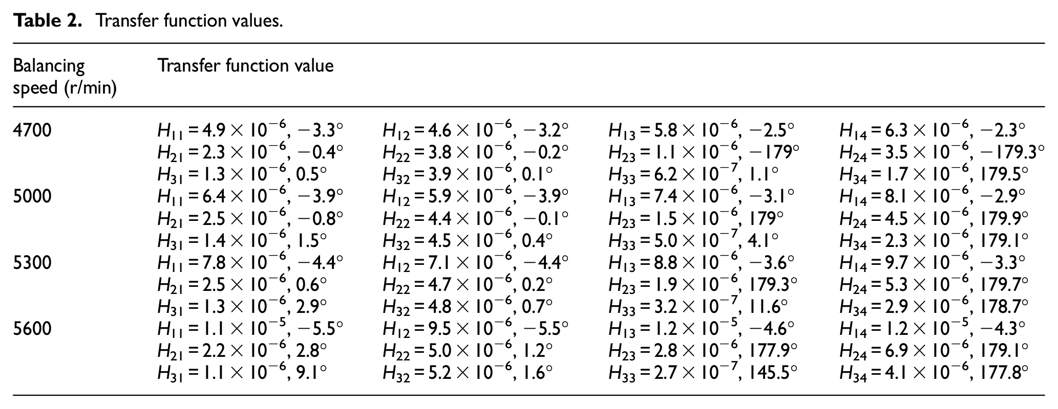
where the first 1 of the $H_{11}$ subscript indicates the measured response of the measurement point 1, the second 1 indicates that the excitation is only input on the equilibrium surface 1, and so on.

The vibration response obtained from the harmonic response analysis, along with the corresponding input excitation, is substituted into the equation (17). The transfer function values at four rotational speeds are then calculated and presented in Table 2.

Table 2.

Transfer function values.

Balancing speed (r/min)	Transfer function value
4700	H ₁₁ = 4.9 × 10⁻⁶, −3.3°	H ₁₂ = 4.6 × 10⁻⁶, −3.2°	H ₁₃ = 5.8 × 10⁻⁶, −2.5°	H ₁₄ = 6.3 × 10⁻⁶, −2.3°
	H ₂₁ = 2.3 × 10⁻⁶, −0.4°	H ₂₂ = 3.8 × 10⁻⁶, −0.2°	H ₂₃ = 1.1 × 10⁻⁶, −179°	H ₂₄ = 3.5 × 10⁻⁶, −179.3°
	H ₃₁ = 1.3 × 10⁻⁶, 0.5°	H ₃₂ = 3.9 × 10⁻⁶, 0.1°	H ₃₃ = 6.2 × 10⁻⁷, 1.1°	H ₃₄ = 1.7 × 10⁻⁶, 179.5°
5000	H ₁₁ = 6.4 × 10⁻⁶, −3.9°	H ₁₂ = 5.9 × 10⁻⁶, −3.9°	H ₁₃ = 7.4 × 10⁻⁶, −3.1°	H ₁₄ = 8.1 × 10⁻⁶, −2.9°
	H ₂₁ = 2.5 × 10⁻⁶, −0.8°	H ₂₂ = 4.4 × 10⁻⁶, −0.1°	H ₂₃ = 1.5 × 10⁻⁶, 179°	H ₂₄ = 4.5 × 10⁻⁶, 179.9°
	H ₃₁ = 1.4 × 10⁻⁶, 1.5°	H ₃₂ = 4.5 × 10⁻⁶, 0.4°	H ₃₃ = 5.0 × 10⁻⁷, 4.1°	H ₃₄ = 2.3 × 10⁻⁶, 179.1°
5300	H ₁₁ = 7.8 × 10⁻⁶, −4.4°	H ₁₂ = 7.1 × 10⁻⁶, −4.4°	H ₁₃ = 8.8 × 10⁻⁶, −3.6°	H ₁₄ = 9.7 × 10⁻⁶, −3.3°
	H ₂₁ = 2.5 × 10⁻⁶, 0.6°	H ₂₂ = 4.7 × 10⁻⁶, 0.2°	H ₂₃ = 1.9 × 10⁻⁶, 179.3°	H ₂₄ = 5.3 × 10⁻⁶, 179.7°
	H ₃₁ = 1.3 × 10⁻⁶, 2.9°	H ₃₂ = 4.8 × 10⁻⁶, 0.7°	H ₃₃ = 3.2 × 10⁻⁷, 11.6°	H ₃₄ = 2.9 × 10⁻⁶, 178.7°
5600	H ₁₁ = 1.1 × 10⁻⁵, −5.5°	H ₁₂ = 9.5 × 10⁻⁶, −5.5°	H ₁₃ = 1.2 × 10⁻⁵, −4.6°	H ₁₄ = 1.2 × 10⁻⁵, −4.3°
	H ₂₁ = 2.2 × 10⁻⁶, 2.8°	H ₂₂ = 5.0 × 10⁻⁶, 1.2°	H ₂₃ = 2.8 × 10⁻⁶, 177.9°	H ₂₄ = 6.9 × 10⁻⁶, 179.1°
	H ₃₁ = 1.1 × 10⁻⁶, 9.1°	H ₃₂ = 5.2 × 10⁻⁶, 1.6°	H ₃₃ = 2.7 × 10⁻⁷, 145.5°	H ₃₄ = 4.1 × 10⁻⁶, 177.8°

Using equation (8), the transfer function matrix is converted into the influence coefficient matrix, which is substituted into equation (7) and solved using WCSSA. The original vibration values are listed in Table 3. The WCSSA parameters are initialized with the following settings: a search lower limit of −50 g, an upper limit of 50 g, a population size of 100, and a total of 400 iterations. Similarly, the four optimization algorithms are solved iteratively using the same parameter settings. The iteration process is shown in Figure 14.

Table 3.

Original vibration values.

Balancing speed (r/min)	Original vibration (m)
4700	$V_{1}^{1}$ = 7.05 × 10⁻⁵, −2.1°; $V_{2}^{1}$ = 6.46 × 10⁻⁵, −179.8°; $V_{3}^{1}$ = 4.85 × 10⁻⁵, 179.8°
5000	$V_{1}^{2}$ = 9.01 × 10⁻⁵, −2.6°; $V_{2}^{2}$ = 7.98 × 10⁻⁵, 179.6°; $V_{3}^{2}$ = 6.07 × 10⁻⁵, 179.6°
5300	$V_{1}^{3}$ = 1.06 × 10⁻⁴, −3.1°; $V_{2}^{3}$ = 9.23 × 10⁻⁵, 179.8°; $V_{3}^{3}$ = 7.09 × 10⁻⁵, 179.4°
5600	$V_{1}^{4}$ = 1.41 × 10⁻⁴, −4.1°; $V_{2}^{4}$ = 1.16 × 10⁻⁴, 179.4°; $V_{3}^{4}$ = 9.05 × 10⁻⁵, 178.9°

Figure 14.

Iteration convergence curve.

The convergence curve indicates that the improved WCSSA demonstrates better adaptability compared to the other four algorithms, both in terms of convergence accuracy and convergence speed. The results stabilize after approximately 50 iterations. Once the stable correction amount is determined, the enumeration method is applied to further refine the solution. Starting from the first stabilized solution and progressing to the last, three measurement points are identified within the solution set. The corresponding counterweight, which minimizes the maximum residual vibration at each measurement point across the four rotational speeds, is then calculated. The final counterweight is presented in Table 4.

Table 4.

Balance weight.

Equilibrium surface 1	Equilibrium surface 2	Equilibrium surface 3	Equilibrium surface 4
6.1 g, 77.3°	13.7 g, −127.8°	7.1 g, −55.4°	7.9 g, −179.9°

After implementing the counterweight scheme outlined in Table 4, the residual vibration is computed using equation (6), and the outcomes are presented in Table 5. Remarkably, the maximum residual vibration measures a mere 1.65 × 10⁻⁵ m.

Table 5.

Counterweight scheme.

Balancing speed (r/min)	Remanent vibration (m)
4700	$R_{1}^{1}$ = 1.65 × 10⁻⁵; $R_{2}^{1}$ = 1.21 × 10⁻⁵; $R_{3}^{1}$ = 8.11 × 10⁻⁶
5000	$R_{1}^{2}$ = 1.19 × 10⁻⁵; $R_{2}^{2}$ = 9.18 × 10⁻⁶; $R_{3}^{2}$ = 1.37 × 10⁻⁵
5300	$R_{1}^{3}$ = 1.49 × 10⁻⁶; $R_{2}^{3}$ = 1.81 × 10⁻⁶; $R_{3}^{3}$ = 4.75 × 10⁻⁶
5600	$R_{1}^{4}$ = 1.11 × 10⁻⁵; $R_{2}^{4}$ = 1.59 × 10⁻⁵; $R_{3}^{4}$ = 2.01 × 10⁻⁶

Experimental verifications

To validate the efficacy and precision of the proposed no-test dynamic balancing optimization method, an experimental test bench is specifically designed and constructed for aero-engine turbine rotors. The configuration of the test bench is illustrated in Figure 15(a). During the preparatory phase of the experiment, eddy current sensors are installed at measurement point 1, 2, and 3 to capture vibration displacement. Acceleration sensors are mounted at supporting points NO.2 and NO.3 for modal testing, as detailed in Section “Dynamics analysis.” Additionally, an eddy current sensor is positioned at a critical phase slot on the shaft to serve as the phase reference sensor. Initial unbalance is introduced by installing a screw weighing approximately 15 g into a threaded hole on the turbine disk, with the mass verified using an electronic balance. Counterweights are applied using detachable screws inserted into threaded holes on the counterweight ring. A magnified view of the counterweight configuration is provided in Figure 15(b). The setup of the signal acquisition system is illustrated in Figure 15(c).

Figure 15.

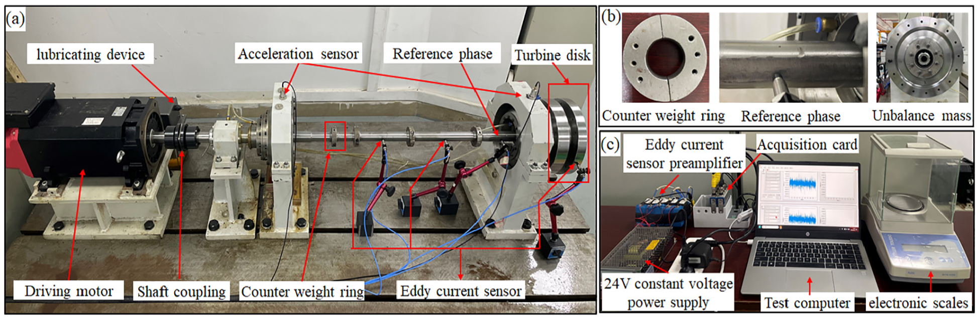
Experimental device: (a) rotor test rig, (b) partial discharge diagram, and (c) test device.

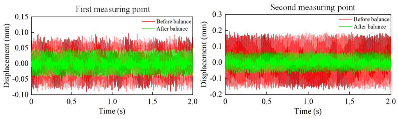
The drive motor is initiated and the rotor speed is gradually increased to 4700, 5000, 5300, and 5600 r/min, respectively, to capture vibration signals after the introduction of unbalanced mass. The sampling frequency is set to 5120 Hz, with a sampling duration of 10 s. Subsequently, the counterweight scheme is fine-tuned by balancing the counterweights on the counterweight clamping ring, taking into account the 30° interval between threaded holes. The final counterweight are adjustments as balance surface 1: (6.1 g, 77°), balance surface 2: (13.7 g, −127°), balance surface 3: (7.1 g, −55°), and balance surface 4: (7.9 g, −180°). After completing these adjustments, the vibration signal acquisition steps are repeated at the same four rotational speeds to collect data post-dynamic balancing. The time-domain vibration signals for measurement points 1 and 2, within the range of 0–2 s, are presented in Figures 16 to 19, corresponding to the conditions before and after the application of dynamic balancing.

Figure 16.

Vibration displacement signal at 4700 r/min.

Figure 17.

Vibration displacement signal at 5000 r/min.

Figure 18.

Vibration displacement signal at 5300 r/min.

Figure 19.

Vibration displacement signal at 5600 r/min.

The above figure clearly demonstrates that, after applying the counterweight balancing scheme, the vibration amplitude at 4700, 5000, 5300, and 5600 r/min is significantly reduced compared to the amplitude observed under unbalanced conditions. This indicates the effectiveness of the proposed dynamic balancing method. The peak-to-peak value of the vibration signal at each speed are measured and summarized in Table 6.

Table 6.

Vibration peak-to-peak value before and after balance.

Revolution speed (r/min)	Before dynamic balance (mm)	After dynamic balance (mm)	Decreasing range (%)
4700	0.3497	0.1780	49.09
5000	0.3648	0.1715	52.93
5300	0.4407	0.1989	54.86
5600	0.4145	0.1933	53.36

Table 6 reveals that, following dynamic balance optimization, the vibration peak-to-peak value is reduced by 49.09% at 4700 r/min, 52.93% at 5000 r/min, 54.86% at 5300 r/min, and 53.36% at 5600 r/min. These results demonstrate the effectiveness of the proposed no-test-weight dynamic balance optimization method in significantly reducing rotor vibration across various operational speeds. Before dynamic balancing, the rotor generates a significant centrifugal force due to the presence of additional unbalanced mass, leading to increased vibration amplitudes at each measurement point. After optimization using the WCSSA method, the unbalanced force is effectively counteracted by the corrective counterweights, resulting in a reduction of the system’s overall centrifugal force and a marked decrease in the vibration response.

Moreover, although the vibration amplitude decreases at all measurement points following dynamic balancing, the extent of reduction varies. This variation is attributed to the positions of measuring points 1 and 2, which are located near the midpoint of the long shaft—corresponding to the anti-nodes of the first and second vibration modes. These positions are more sensitive to unbalanced excitation, thereby exhibiting more substantial reductions in vibration amplitude after dynamic balancing.

To quantify the balancing effect, the dynamic balance method proposed in this study is applied after removing all initial counterweights from the system. A high-speed rotor dynamic balance instrument (Jiangsu Lianyi You Measurement and Control Technology Co., Ltd.) is used to perform the correction in compliance with the ISO 21940-11 standard. The high-speed rotor dynamic balance system utilized in the experiment is shown in Figure 20.

Figure 20.

High-speed rotor dynamic balance instrument.

The comparison scheme utilizes the control variable method to ensure that both balancing experiments are conducted under identical operating conditions. The peak-to-peak vibration amplitudes before and after dynamic balancing are recorded in Table 7 for comparative analysis.

Table 7.

Vibration peak-to-peak value before and after weighing.

Rotating speeds (r/min)	Field dynamic balance (mm)
4700	0.1978
5000	0.2054
5300	0.2275
5600	0.2264

The comparison reveals that the proposed dynamic balance correction method achieves an average vibration amplitude reduction of 52.56%, which is better than the 45.23% vibration attenuation of the traditional field dynamic balance method. In addition to higher efficiency, the method also enhances accuracy, further validating its effectiveness.

Conclusion

This study presents a dynamic balance optimization method for high-speed aero-engines rotors, based on the WCSSA. By integrating virtual prototype modeling, transfer function balancing technique, and the WCSSA, the proposed approach effectively enhances the reduction of residual vibration after balancing. Experimental verification substantiates the following conclusions:

(1) The improved WCSSA is specifically adapted for dynamic balancing problems involving multiple rotational speeds, measurement points, and balance surfaces. It improves convergence speed and optimization accuracy. A correction optimization framework based on model prediction is developed, which minimizes the need for trial runs and reduces system downtime—effectively overcoming the limitations of traditional trial-and-error methods reliant on manual experience.

(2) The WCSSA-based optimization method significantly reduces residual vibrations across all rotational speeds. When multiple solutions yield identical maximum residual vibrations under the same counterweight scheme, an enumeration strategy is employed to determine the final counter-weight configuration that minimizes the maximum residual vibration at each measurement point.

(3) The proposed method effectively mitigates excessive rotor vibration caused by mass imbalance. Experimental results demonstrate substantial reductions in peak-to-peak vibration amplitudes across different speeds: 49.09% at 4700 r/min, 52.93% at 5000 r/min, 54.86% at 5300 r/min, and 53.36% at 5600 r/min, confirming the efficacy of the optimization strategy without the need for test weights.

Footnotes

Handling Editor: Divyam Semwal

ORCID iDs

Changzhi Shi

Hui Ma

Funding

The author(s) disclosed receipt of the following financial support for the research, authorship, and/or publication of this article: This work was supported by the National Natural Science Foundation of China (Grant No.12072076, Grant No.52275094) and Guangdong Provincial Program for Innovative Teams in Ordinary Universities (2023KCXTD031).

Declaration of conflicting interests

The author(s) declared no potential conflicts of interest with respect to the research, authorship, and/or publication of this article.

References

Zhao

Gao

Cheng

, et al. Reliability study on the fatigue life of film cooling blades in advanced aero-engine turbines: neglected crystal orientation uncertainty in casting. Aerosp Sci Technol 2022; 130: 107880.

Mei

Sun

, et al. Research on intelligent assembly method of aero-engine multi-stage rotors based on SVM and variable-step AFSA-BP neural network. Adv Eng Inform 2022; 54: 101798.

Zhang

Liu

Recent progress in precision measurement and assembly optimization methods of the aero-engine multistage rotor: a comprehensive review. Measurement 2024; 235: 114990.

Liu

Liao

, et al. Conceptual design and optimization of polymer gear system for low-thrust turbofan aeroengine accessory transmission. J Comput Des Eng 2024; 11(1): 212–229.

Han

Yang

Zhu

, et al. Unbalance position of aeroengine flexible rotor analysis and identification based on dynamic model and deep learning. Proc IMechE, Part C: J Mechanical Engineering Science 2023; 237(19): 4410–4429.

Jin

Zhou

Quan

, et al. Topological structures of vibration responses for dual-rotor aeroengine. Mech Syst Signal Process 2024; 208: 111053.

Deng

Tong

Zheng

, et al. Investigation on transient dynamic balancing of the power turbine rotor and its application. Adv Mech Eng 2021; 13(4): 16878140211007325.

Cao

, et al. Review of rotor balancing methods. Machines 2021; 9(5): 89.

Moon

J-D

Kim

B-S

Lee

S-H.

Development of the active balancing device for high-speed spindle system using influence coefficients. Int J Mach Tools Manuf 2006; 46(9): 978–987.

10.

Han

D-J.

Generalized modal balancing for non-isotropic rotor systems. Mech Syst Signal Process 2007; 21(5): 2137–2160.

11.

Bin

Shen

, et al. Development of whole-machine high speed balance approach for turbomachinery shaft system with N+ 1 supports. Measurement 2018; 122: 368–379.

12.

Khulief

Mohiuddin

El-Gebeily

A new method for field-balancing of high-speed flexible rotors without trial weights. Int J Rotating Mach 2014; 2014(1): 603241.

13.

Zhao

Ren

Deng

, et al. A transient characteristic-based balancing method of rotor system without trail weights. Mech Syst Signal Process 2021; 148: 107117.

14.

Sanches

Ap Cavallini

Jr Steffen

Jr.

Theoretical and experimental applications of a rotor balancing technique without using trial weights based on augmented Kalman filter. Mech Syst Signal Process 2024; 208: 111066.

15.

Xie

D-M

Yang

Liu

Z-H

, et al. A balance method without trial mass based on lag phase. In: Proceedings of the ASME international mechanical engineering congress and exposition, San Diego, CA, USA, 15–21 November 2013.

16.

Ranjan

Tiwari

On-site high-speed balancing of flexible rotor-bearing system using virtual trial unbalances at slow run. Int J Mech Sci 2020; 183: 105786.

17.

Wang

Hou

, et al. Balancing method without trial weights for rotor systems based on similitude scale model. Front Mech Eng 2018; 13: 571–580.

18.

Yao

Yang

, et al. Balancing optimization of a multiple speeds flexible rotor. J Sound Vib 2020; 480: 115405.

19.

Zhong

Chen

, et al. A novel balancing method for rotor using unsupervised deep learning. Shock Vib 2021; 2021(1): 1800164.

20.

Garpelli

Alves

Cavalca

, et al. Physics-guided neural networks applied in rotor unbalance problems. Struct Health Monit 2023; 22(6): 4117–4130.

21.

Zhang

Xuejun

Qingkai

, et al. Research on dynamic balance optimization method of flexible rotor based on GWO. Meas Sci Technol 2024; 35: 106108.

22.

Briend

Chatelet

Dufour

, et al. Dry-whip phenomenon in on-board rotordynamics: modeling and experimentation. J Sound Vib 2021; 513: 116398.

23.

Luo

Liu

, et al. Dynamic modeling and stability analysis of a rotor-bearing system with bolted-disk joint. Mech Syst Signal Process 2021; 158: 107778.

24.

Tiwari

Rotor systems: analysis and identification. CRC Press, 2017.

25.

Xue

Shen

A novel swarm intelligence optimization approach: sparrow search algorithm. Syst Sci Control Eng 2020; 8(1): 22–34.

26.

Cao

Mao

Zhou

Designing a 2D infinite collapse map for image encryption. Signal Process 2020; 171: 107457.

27.

Mirjalili

Lewis

The whale optimization algorithm. Adv Eng Softw 2016; 95: 51–67.

28.

Zhao

Fang

Liu

, et al. A covariance-based Moth–flame optimization algorithm with Cauchy mutation for solving numerical optimization problems. Appl Soft Comput 2022; 119: 108538.

29.

Trojovský

Dehghani

Subtraction-average-based optimizer: a new swarm-inspired metaheuristic algorithm for solving optimization problems. Biomimetics 2023; 8(2): 149.

30.

Xue

Shen

Dung beetle optimizer: a new meta-heuristic algorithm for global optimization. J Supercomput 2023; 79(7): 7305–7336.

31.

Abdollahzadeh

Soleimanian Gharehchopogh

Mirjalili

Artificial gorilla troops optimizer: a new nature-inspired metaheuristic algorithm for global optimization problems. Int J Intell Syst 2021; 36(10): 5887–5958.

32.

Mohamed

Hadi

Agrawal

, et al. Gaining-sharing knowledge based algorithm with adaptive parameters hybrid with IMODE algorithm for solving CEC 2021 benchmark problems. In: Proceedings of the 2021 IEEE congress on evolutionary computation (CEC), Kraków, Poland, 28 June–1 July 2021.

33.

Lee

H-H.

Finite element simulations with ANSYS workbench 2023: theory, applications, case studies. SDC Publications, 2023.

Dynamic balance optimization method for aero-engine rotor without trial weight

Abstract

Keywords

Introduction

Dynamic balancing optimization method

The principle of dynamic balance

WCSSA optimization algorithm

WCSSA algorithm verification

Design process of dynamic balance optimization

Example of dynamic balance

Virtual prototype modeling

Dynamics analysis

Dynamic balance optimization method based on WCSSA

Experimental verifications

Conclusion

Footnotes

ORCID iDs

Funding

Declaration of conflicting interests

References