
Abstract
Internal Combustion (IC) engines are commonly used in the process industry, and proper Air-Fuel Ratio (AFR) regulation in their fuel system is essential for improved engine performance, fuel efficiency, and environmental protection. Since faults in the sensors of the AFR system cause the engine to shut down, fault tolerance is essentially required for them. In this paper, an advanced Active Fault-Tolerant Control System (AFTCS) for AFR control of an IC engine is proposed to prevent the engine shutdown. For analytical redundancy, the proposed AFTCS uses the Genetic Algorithm (GA) based observer model in the Fault Detection and Isolation (FDI) unit to generate estimated value for the faulty sensors using the values of other healthy sensors. The proposed framework was simulated in the MATLAB/Simulink environment to verify its effectiveness. In comparison to previous literature works, the results show that the AFR control system has superior fault tolerance output for sensor faults, especially for the MAP sensor, in terms of less oscillatory response. Finally, a comparison of the proposed GA-based AFTCS was carried out with the existing literature works and its superior performance was elaborated.
Keywords
Introduction
A system fault is characterized as a deviation of the parameter from its actual value. Fault tolerance refers to a system’s ability to continue operating in defective conditions. Any real-world machine can develop faults, which reduce the system’s stability and efficiency.1–3 Fault-tolerant control (FTC) is a technique that can be used to improve the stability of sensitive systems like nuclear power plants and airplanes. The two most common forms of FTC are active and passive.4–6 The Active Fault-Tolerant Control System (AFTCS) comprises a Faut Detection and Isolation (FDI) unit that is responsible for detecting and isolating defective system components. The FDI employs the observer principle, in which a plant parameter is compared to a predefined normal value to provide a residual. 7 If the residual is below reasonable limits, the system is said to be free of errors. If the residual exceeds the specified threshold, the FDI unit declares faulty conditions. 8 The controller is then reprogramed to meet the new operational requirements. Output may be harmed by defective parts, but overall system reliability is assured.9,10
An FDI unit can be built using several approaches. For example in Amin and Mahmood-ul-Hasan, 2 Kalman Filter (KF) is used and in general, the KF is not an ideal estimator. The measurement and the state transition model should both be linear for a KF to generate accurate estimations but the model used in Amin and Mahmood-ul-Hasan 2 is nonlinear hence KF is generating less accurate values. A linear regression-based model is used in Amin and Mahmood-ul-Hasan, 11 Linear Regression Algorithm is too conventional, hence when used for the estimation of a nonlinear sensor it is showing poor performance. An Artificial Neural Network (ANN)-based approach is reported in Shahbaz and Amin 12 which is showing highly accurate results but the critical data points on which the error percentage is high are ignored in that study. The model reported in Berredjem and Benidir 13 is using fuzzy logic to diagnose the bearing faults. The study reports a high degree of accuracy but there is a systematic approach to applying Fuzzy Logic to solve a problem. As a result, several solutions to a single problem emerge, confusing. Furthermore, the control system built in Berredjem and Benidir 13 must be updated on a regular basis.
In an aero-engine, KFs are used in Yuan et al. 14 for fault detection and position in the case of sensor and actuator faults coexisting. In Berredjem and Benidir, 13 FDI employs fuzzy logic to forecast nonlinear processes, while adaptive control is used to correct bias and locate actuator faults. Using simulated sensor values in FDI to estimate flow speeds for actuator faults, a nonlinear adaptive observer for a double pipe heat exchanger is built. 15 FTC was important in designing a control strategy in quasi and procedure environments in flawed scenarios. FTC is a key component in maintaining system reliability and stability when it comes to actuator and sensor faults. 16 configures multilevel reconfiguration for actuators and sensors using the NASA aircraft LPV system. In a recent configuration of the drone control system, NASA has used FTC. 17 To achieve good orbit-attitude tracking performance an improved finite-time sliding mode control approach is proposed in Shi et al. 18 in which the soft docking procedure is separated into three sequential movements with set duration to reduce the complexity, and the high-precision performance of the generated simplified electromagnetic force/torque models is shown by numerical analysis. Another study related to spacecraft docking can be found in Zhang et al. 19 in which the essential problems in spacecraft electromagnetic docking control, such as model uncertainties, unknown external disturbances, and inherent strong nonlinearity and coupling, are solved using a nonlinear sliding mode control that combines online model modification, a nonlinear sliding mode controller, and a disturbance observer. In Liu et al., 20 Delayed Electromagnetic Docking of Spacecraft in Elliptical Orbits with Active Disturbance Rejection Control is proposed and validated with a high degree of accuracy however the non-fragile control dealing with controller perturbations is not considered in this study. The authors Maki et al. 21 have suggested a multi-controller solution without using an FDI decision-making unit. In Yang and Yin, 22 a hybrid solution was proposed for restoring sensor values using simulated sensor values to ensure reliability in the event of sensor failure. To define the affected variables, the proposed FDI scheme in Li et al. 23 uses the canonical variate analysis (CVA) technique and the exponentially weighted moving average (EWMA) paradigm based on Pearson correlation analysis. Some more nonlinear fault-tolerant control systems are reported in the literature, a proportional-integral observer is used for Switched Fuzzy Stochastic Systems in Han et al., 24 and a directed-graph based approach is reported in Han et al. 25 in which a unique intermediate observer design approach is provided to estimate system states, actuator failures, and sensor faults. Another nonlinear fault estimation approach can be found in Han et al. 26 in which a dynamic proportional-integral observer is used for nonlinear system. In Han et al.,24,26 a P-I controller is used and as stated in Sreekumar and Jiji 27 the P-I controller has some drawbacks, including a large initial overshoot, sensitivity to controller gains, and a slow reaction to unexpected disturbances, hence an improved control strategy is necessary. In Han et al. 25 directed graphs are used and for directed graphs, the memory complexity is quadratic due to which this approach will be less effective for devices with memory constraints. If complete data measurements are inaccessible, Ding and Fang 28 proposed an FDI approach that deals with intermittent observations. In a case study, Yu et al. 29 looked at performance degradations induced by incipient faults and estimated the residual existence of a mechatronic system. To increase the monitored system’s separation capability when multiple faults occur, two analytical redundancy relations were addressed.
It is quite evident from the literature that the existing models for the AFR control of an IC engine are either using the lookup tables, linear regression, KF, or ANN. Linear regression is a very basic technique and is less accurate. Lookup tables and ANN techniques are computationally less efficient and KF is limited to the linear region of the sensors. Some other techniques are also using some advanced algorithms like SVM, deep learning, CVA, or EWMA. But in these advanced techniques, we need a large dataset. Our contribution to this research is the implementation of a GA-based observer model in the FDI unit. The proposed method is producing excellent results (up to 77% improvement in the standard error of estimation) despite having a limited dataset. The proposed method uses very basic GA which tends to find the local optimum solution and can be used on the hardware with limited computational power or in time-critical applications. In comparison to previous literature works, the simulation results show superior fault tolerance efficiency, particularly for the MAP sensor, in terms of less oscillatory response.
The rest of the paper is organized in the following order. Problem formulation and computation of fitness functions are presented in section 2, section 3 is explaining results and finally, the paper is concluded in section 4.
Research methodology
Using the available AFR model 30 of the IC gasoline engine, the proposed AFTCS was implemented in MATLAB/Simulink. For analytical redundancy, the proposed AFTCS uses the Genetic Algorithm (GA) based observer model in the Fault Detection and Isolation (FDI) unit to generate estimated value for the faulty sensors using the values of other healthy sensors. The Fault Injection Unit (FIU) sends a fault to each sensor one at a time, leaving the others unaffected. The engine speed is set to 300 rpm for this analysis based on the MATLAB model’s design speed. We have used constant speed in this research work as the engines mostly run at constant speed in the process plant, and the 300 rpm of speed is provided to a controller by the design FDI when the speed sensor stops working. Load variations and their impact on speed are not considered as the paper is more focused on developing GA-based AFTCS. The modeling and development of the system are further explained in the next subsections:
Air-fuel ratio control
An Internal Combustion (IC) engine is a heat engine that uses air to help burn fuel in a combustion chamber. In production processes, IC engines are commonly used as prime movers. Chemical energy is translated into mechanical rotation, which is then used to power the engines’ compressors and alternators. Compression-ignition (CI) and spark-ignition (SI) engines are the two types of IC engines. The compression causes combustion in CI engines, while spark plugs cause combustion in SI engines. The Air Fuel Ratio (AFR) is a calculation of how much air and fuel are combined in a certain ratio during the combustion process. The general architecture of the air-fuel ratio (AFR) of an SI IC engine is shown in the Figure 1.
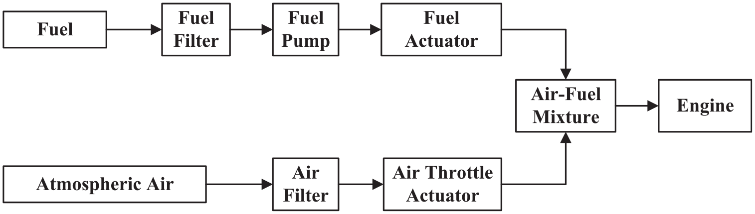
Architecture of Air-fuel System of SI IC Engine. 5
The mathematical equation of AFR is:
The chemical equation is given as:

In this equation, the AFR is referred to as the stoichiometric ratio, and its value for gasoline is 14.6:1. The AFR can range from 6:1 to 20:1 depending upon the type of fuel. A rich mixture has a lower AFR value than the stoichiometric ratio and a lean mixture has a higher AFR value than the stoichiometric ratio. For example, the 16.5:1 AFR is lean, while the 13.7:1 AFR is rich in gasoline. Rich and lean mixtures are also hazardous to the engine because they weaken the catalyst and reduce engine performance and efficiency.2,33
Four sensors play an important role in maintaining AFR control of the SI IC engines:
An engine shut down can be caused due to faults in the above-mentioned sensors, hence fault tolerance is required. It is desirable to generate virtual redundant sensors in the FDI unit that have a nonlinear response like actual sensors. That is why we have used the GA technique in AFTCS architecture to approximate the system. For the speed sensor fault, we supplied the operating speed of the engine to the FDI unit. For relay type EGO sensor, we supplied 12 V to the FDI unit as zero value comes in the operating range which is from 0 to 1 V. The GA-based observers were built for the MAP and Throttle sensors. MATLAB model lookup tables 31 were used to extract the MAP and throttle sensor data for 300 rpm.
Genetic algorithm
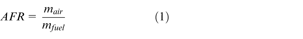
The genetic algorithm (GA) is a search heuristic algorithm inspired by evolutionary theory. We often use GA to look at alternatives to optimization issues. Genetic algorithms are appropriate for massive search spaces and NP-complete problems. We create several generations to achieve the final solution by GA, and the fittest generation has a better chance of surviving in the next generation. 32 The generations of the current population go through crossover and mutation cycles. Each generation has a solution, and the most appropriate or applicable generation is chosen as the final solution. The GA operations are shown in Figure 2.
Genetic algorithm operations.
The steps performed while applying the genetic algorithm to an optimization problem are given below.
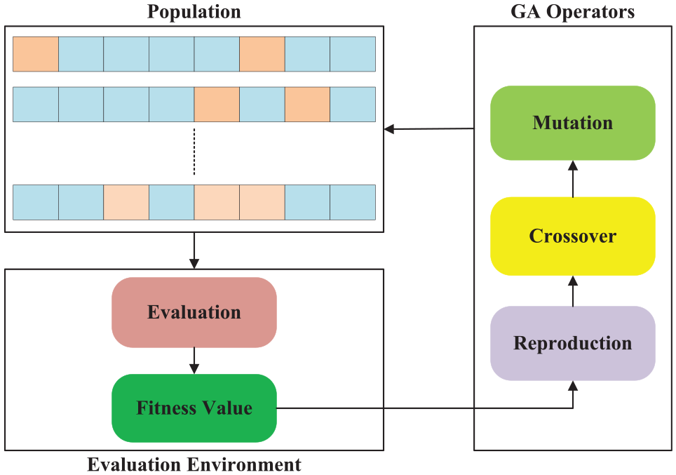
The evolution process normally begins with a population of randomly generated individuals and proceeds in an iterative manner, with each iteration’s population being referred to as a generation. Every set of values in the population is assessed in each generation; fitness is normally the value of the objective function in the optimization problem being solved. Once the first generation is evaluated, the next step is to generate the second-generation population. Crossover (also known as recombination) and mutation are two genetic operators that are used to pick a population of solutions. This process continues until an optimal solution is achieved or the termination condition is met. The common termination conditions are:
An optimum solution is achieved.
A fixed number of generations are reached.
Computation time has reached to maximum allocated limit.
The fitness of the highest-ranking solution is approaching or has reached a point where subsequent iterations no longer yield improved outcomes.
Combination of above-listed conditions.
The overall working of the genetic algorithm can be seen in Figure 3.
Flowchart of genetic algorithm.
Due to its impressive performance, GA is widely used in optimization and classification problems ranging from fault diagnosis in PV cells, 33 OFDM and OQAM synchronization estimation, 34 OFDM modulation, 35 classification problem solving, 36 hyperparameter optimization of power amplifiers, 37 optimal resource allocation in cloud computing, 38 linear array antenna designing, 39 robotic locomotion optimization, 40 compressor-based system’s slow speed characteristics estimation, 41 and many more similar problems. In this study, we are using the genetic algorithm to predict the estimated values in case of a faulty MAP or throttle sensor in an AFTCS.
We can see from the literature that most of the work on fault detection uses Kalman filters, lookup tables, linear regression, ANN, machine learning, or fuzzy logic. For the nonlinear sensors, linear regression yields less reliable sensor values, while the Kalman filters and lookup table approaches are time-consuming. Computational capacity is needed for methods such as ANN, machine learning, and fuzzy logic. As a result, we have suggested a genetic algorithm-based AFTCS for extremely nonlinear sensors in an IC engine’s AFR system. The suggested methodology is both computationally and time-efficient without sacrificing precision.
Moreover, the traditional calculus-based methods work in the problems in which we start at a random point and go in the direction of the gradient until we reach the top of the hill. This method is fast and effective when dealing with single-peaked objective functions, such as the cost function in linear regression. However, in most real-world scenarios, like finding the optimal estimated values of nonlinear sensors in case of a failure, we face a dynamic problem known as landscapes, which consists of several peaks and valleys, causing certain approaches to fail because they have an intrinsic propensity to get trapped at the local optima. Hence we need a more versatile technique like GA to find the optimal solution for these sorts of problems.
System modeling
There are many types of air-fuel ratio control dynamics, including air dynamics, fuel dynamics, sensor model, and controller configuration. 42 Each dynamics’ formulation is given here.
Air dynamics
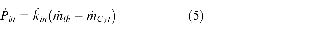
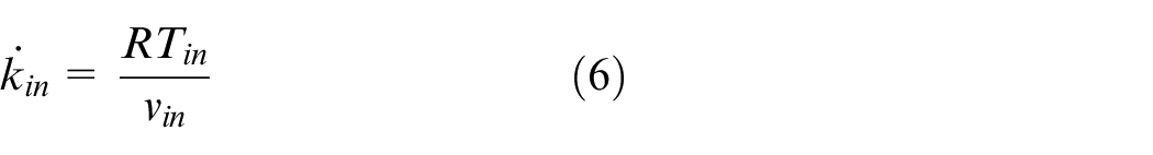
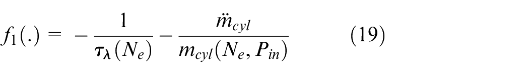
Using the theory of mass conservation and the ideal air gas hypothesis, the air intake dynamics are described as follows:
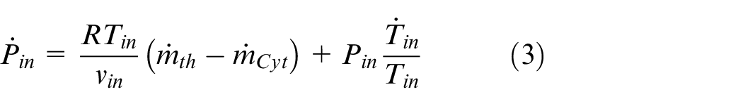

In the above equations,
with
The air mass flow through the valve is 43 :
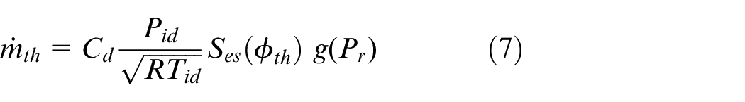

Where
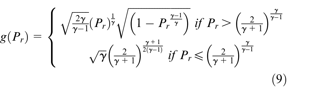
Here γ is the air heat ratio and its value is considered to be 1.4.
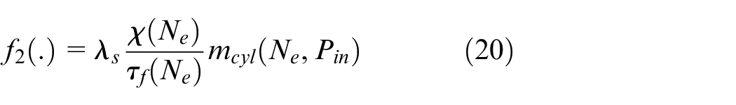
Fuel Dynamics
The fuel dynamics are well demonstrated in Sui and Hall 44 as:
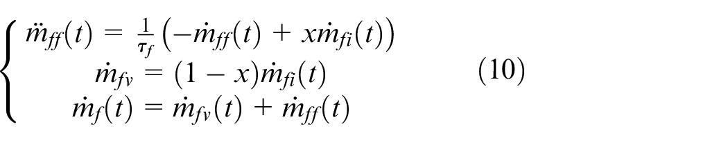
Where


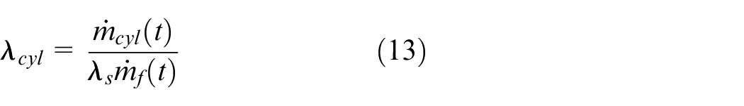
The AFR will now become:
Sensor model
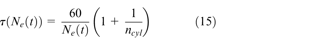
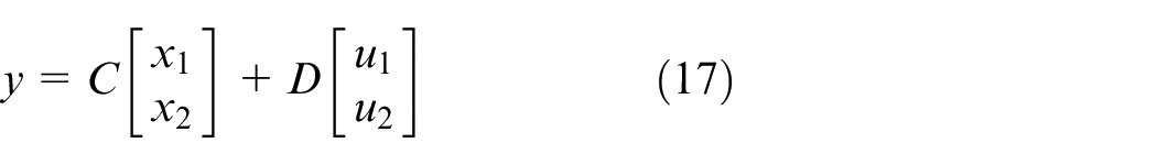
The expression of lambda (λ) sensor model is given by:
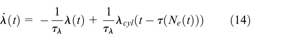
Here τλ is the fixed time delay and its value is 0.1 s.
An engine speed
State space representation
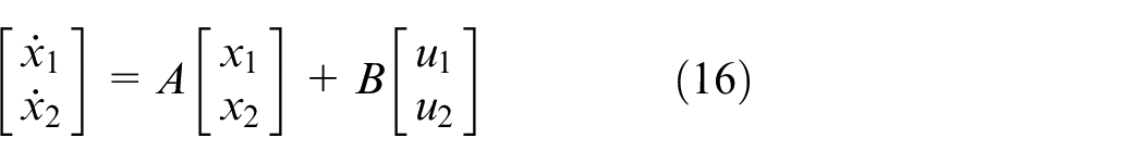
We can represent the state-space model as:
With
Bounded as follows:
Controller design
In Wang et al. 46 have demonstrated the working of AFTCS in state-space. We are using the same to explain the architecture of observer,


where x is the state vector, u is the input vector and y is the output vector. A, B, C, and D are system matrices.


In (24), L is the feedback gain.


FDI will not declare any fault when the residual “
The non-linear observer design equation we get from (27) is.

“g(x,u,t)” is a nonlinear function and is assumed to be globally Lipschitz.
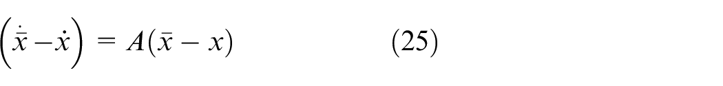
Let

From equations (33) and (34), we get.

The reliability of each sensor is denoted by R.
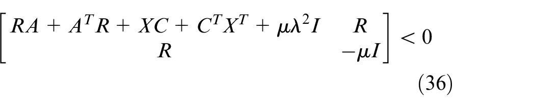
The observer gain matrix can be selected as follows:

By considering the following Lyapunov function to prove its derivative to be zero we can justify the choice of observer gain matrix:

Now we will check
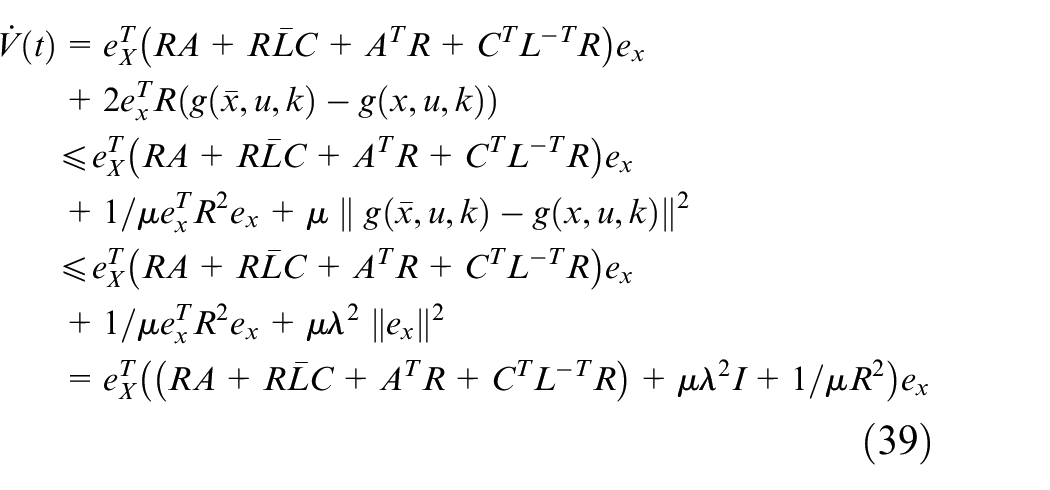
Substituting (38) in (39) we get:
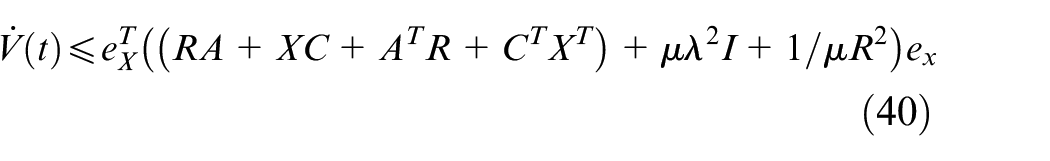
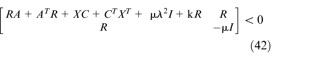
If the following inequality holds,
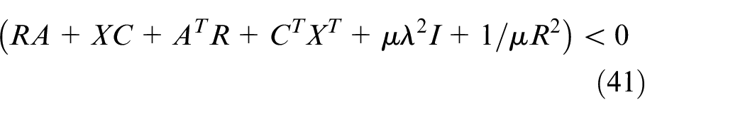
This inequality becomes equal to (36) by applying Schur complement, which completes the proof.
To prove this, consider (40) and (42) to get

Hence, we can write

From (38) we get

Where
Coming back to the residual equation:

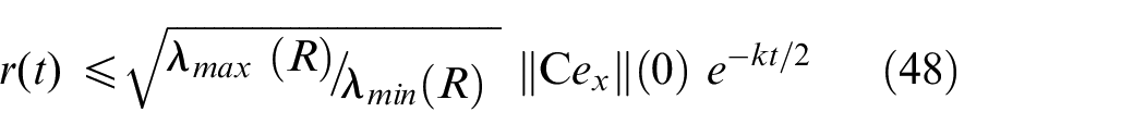

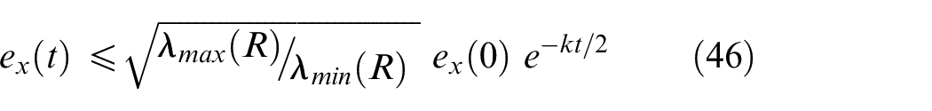
Finally, we can come up with the following criteria for fault detection of a sensor fault.
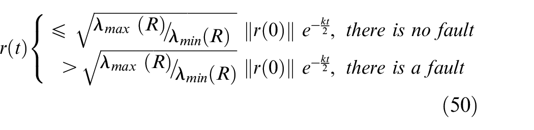
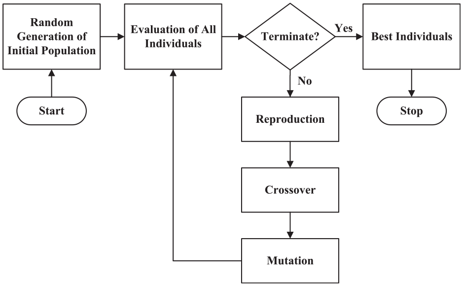
Figure 4 depicts the working of the proposed AFTCS.
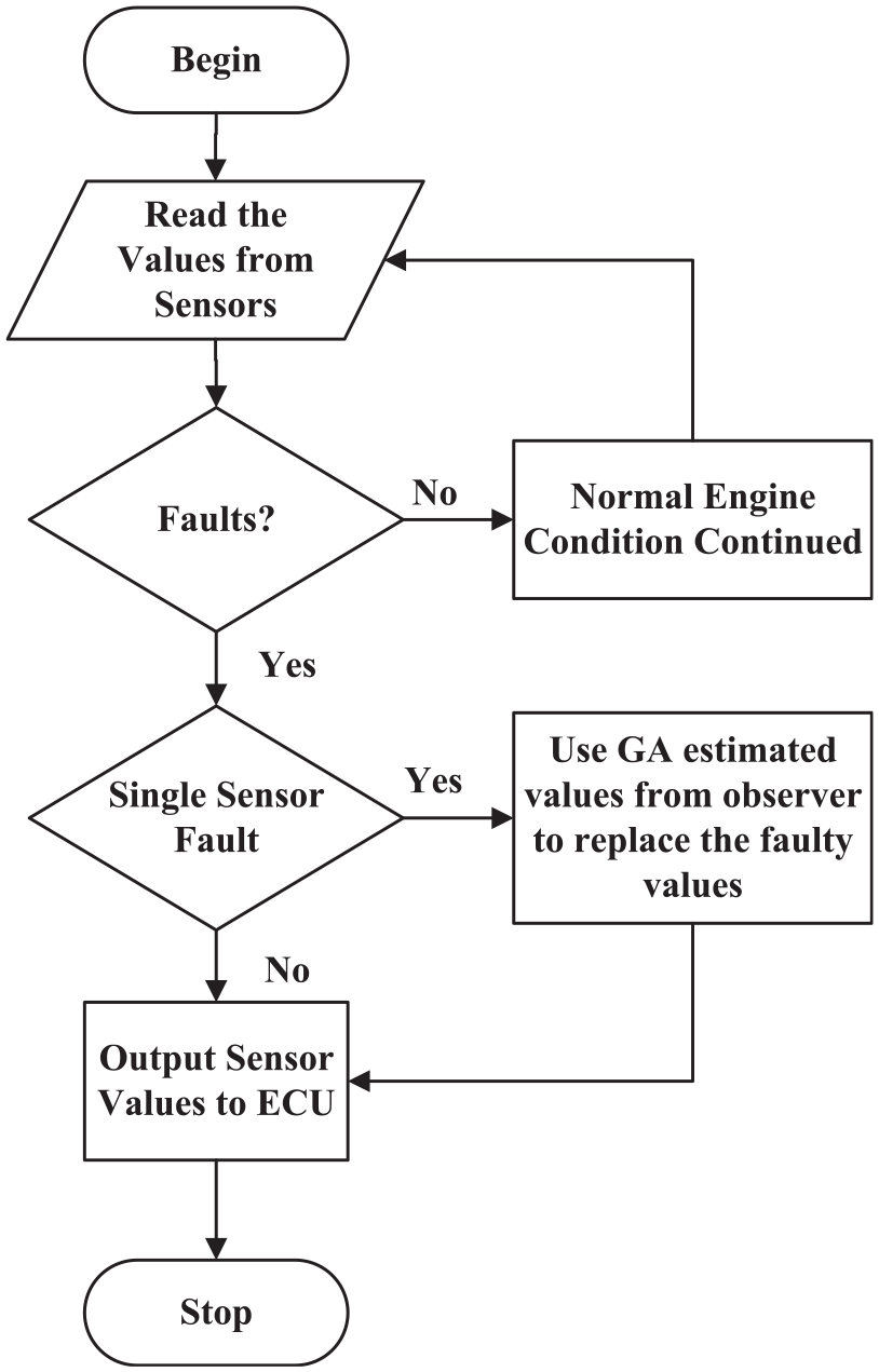
Proposed FTCS’ Flowchart.
The sensor values are tested and the sensor-to-observer value threshold
If
If
The engine works as expected if there is no fault. When a single sensor fails, the error signal, on the other hand, exceeds the threshold. To replace the faulty sensor value, the FDI unit feeds the Engine Control Unit (ECU) an estimated value derived from the observer model based on GA. The contribution of the estimated simulated value of the faulty sensor provides analytical redundancy to the model.
Fitness function formulation
In order to utilize the GA for the estimation of faulty sensor values, we need the fitness function. In this section, the mathematical formulation of fitness functions for the MAP and throttle sensor estimations is given.
Fitness function for MAP estimation
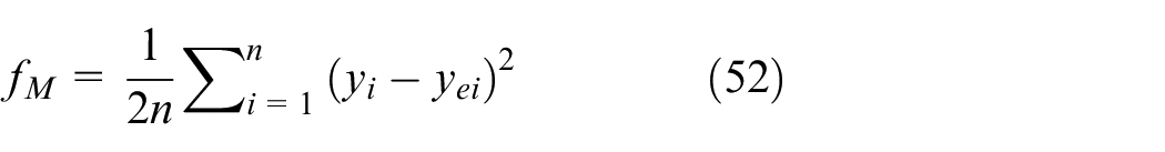
To formulate the fitness function for the MAP estimation the sum of the least-squares method is used. An exponential equation given by (51) is used to predict the values of MAP sensors in case of a fault.

Here ye is the estimated MAP value, x is throttle angle, a and b are unknown constants. The difference between estimated MAP value (ye) and actual MAP value (y) is calculated and the sum of difference over the entire range of x is computed to find the fitness function fM. The expression for the fitness function is given as.
Using (51) in (52), we get
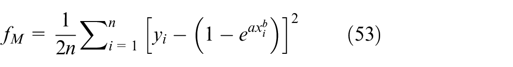
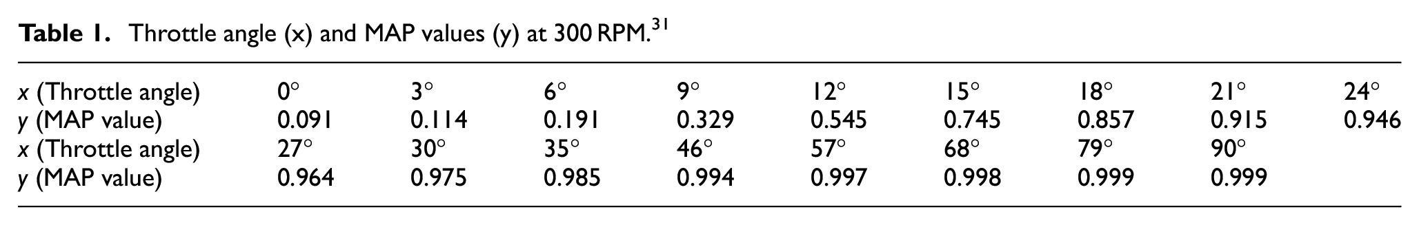
Here n = 17, and the values of x and y are given in Table 1 below.
Throttle angle (x) and MAP values (y) at 300 RPM. 31
The fitness function given by (53) is then minimized by using GA to find the best possible values of the unknown coefficients “a” and “b.”
Fitness function for throttle estimation
To formulate the fitness function for the throttle estimation the sum of the least-squares method is used. A polynomial of fourth order given by (54) is used to predict the values of throttle angle in case of a fault.

Here ye is the estimated throttle value, x is MAP value, a, b, c, d, and e are unknown constants. The difference between estimated throttle angle (ye) and actual throttle angle (y) is calculated and the sum of difference over the entire range of x is computed to find the fitness function fT. The expression for the fitness function is given as.
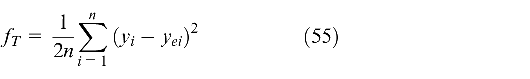
Using (54) in (55), we get
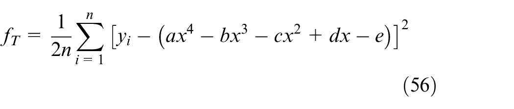
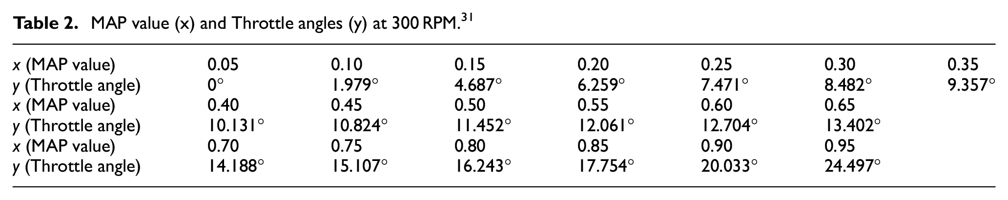
Here n = 19, and the values of x and y are given in Table 2 below.
MAP value (x) and Throttle angles (y) at 300 RPM. 31
The fitness function given by (56) is then minimized by using GA to find the best possible values of the unknown coefficients a, b, c, d, and e.
Despite having good performance, the GA has some limitations which are listed below.
The GA used in this study is only suitable for the fitness functions of moderate complexity. If the fitness function is complex or too simple, then GA efficiency will be very low in terms of computation time and resources usage.
The solution generated by GA is relatively better than the other solutions computed in GA, so we need to repeatedly plot the actual and estimated results.
For multivariable fitness functions the GA sometimes generates the local minima, so we need to adjust the range of solution values accurately.
Despite these limitations, we have used GA over the other techniques due to following reasons.
Unlike other optimization algorithms like Particle Swarm Optimization (PSO), GA is discrete and is used for the problems in which we have a discrete set of data. 48 In our case, we have used the finite set of values for the MAP and throttle sensors so GA is more suitable here.
GA finds the local maxima/minima instead of finding the global optimum solution 48 hence it tends to provide the solutions more quickly.
We have considered the full type sensor faults in this study and assumed that the sensor becomes a short circuit in a faulty condition. The partial type faults in which the sensor does not become fully faulty rather gives partial output are not considered as a limitation of the study. Moreover, zero switching time is assumed in the sensor switches process. Practically, a certain time delay occurs in the switching process.
Results and discussion
Fitness function optimization with GA
MAP estimation
The fitness function given by (53) is minimized to find the best possible values of unknown coefficients “a” and “b” by using the GA function in MATLAB. With the default settings of GA, the results were not satisfactory, so the GA parameters were changed to get suitable results. As the fitness function was having several minimums, so to find the optimum minimum, the number of generations was kept to 50, and the range of values was set to [0.001, 2]. With these settings the values of “a” and “b” are found to be:

The fitness function value for each generation and the mean fitness values along with the best individual values of “a” and “b” are shown in Figure 5.
GA results for MAP estimation.
Once the fitness function is minimized and the optimum values of unknown coefficients are found, the estimated values are found by using MATLAB. The relation between original and estimated values is elaborated by the line fit plot as given below in Figure 6.
Line fit plot for original and estimated MAP sensor values.
In Figure 6, the R2 is equal to 0.987 and we can notice that the estimated values are very close to the original values which proves the efficiency of GA for the estimation of MAP values. We can also notice from Figure 5 the GA reached its optimum solution very quickly and it took only 42 generations to minimize the fitness function of the MAP sensor.
Throttle estimation
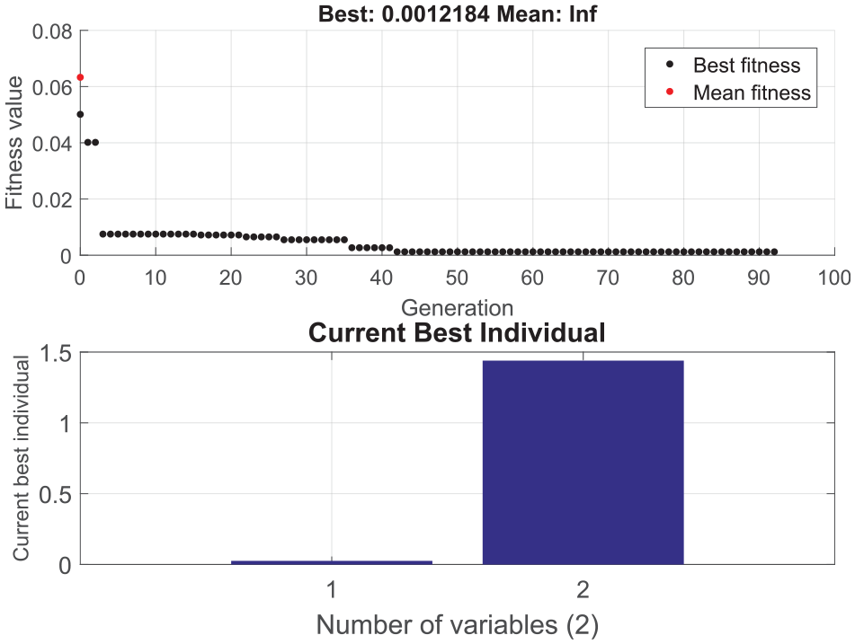
The fitness function given by (56) is minimized to find the best possible values of unknown coefficients “a,”“b,”“c,”“d,” and “e” by using the GA function in MATLAB. With the default settings of GA, the results were not satisfactory, so the GA parameters were changed to get suitable results. As the fitness function was having several minimums, so to find the optimum solution, the number of generations was kept to 250, and the range of parameter values was set to [40, 60]. With these setting the values of “a,”“b,”“c,”“d” and “e” is found to be:
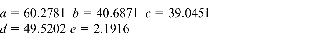
The fitness function value for each generation and the mean fitness values along with the best individual values of unknown coefficients are shown in Figure 7 below.
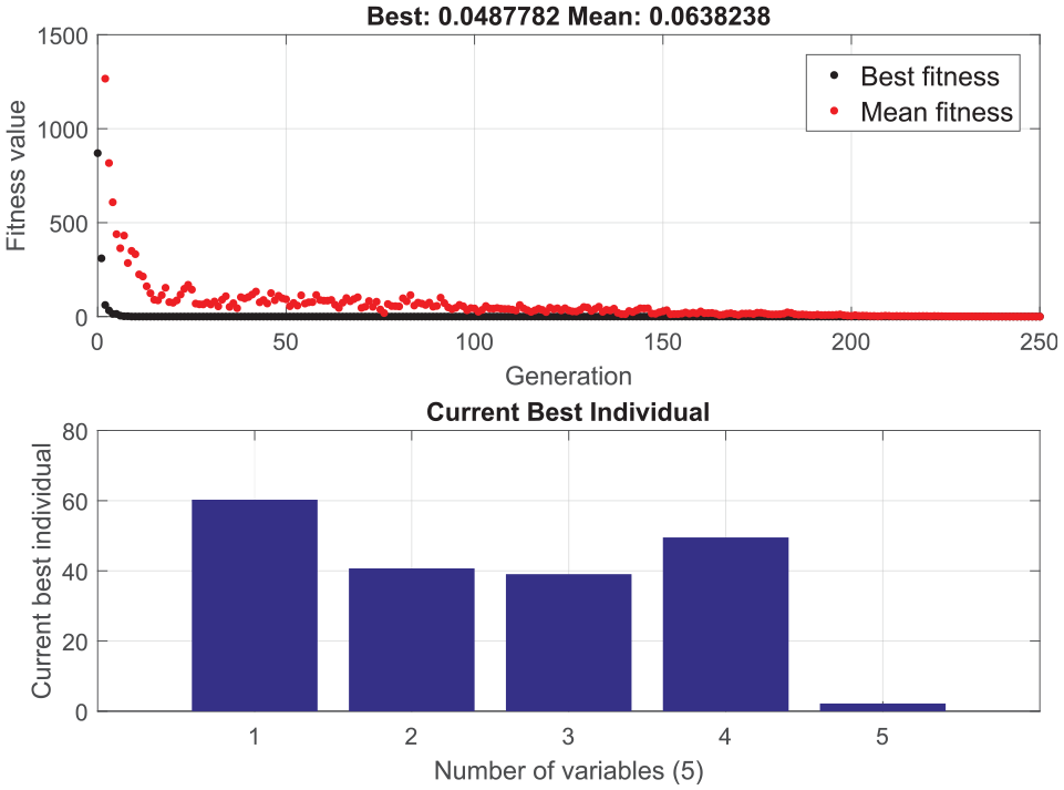
GA results for throttle estimation.
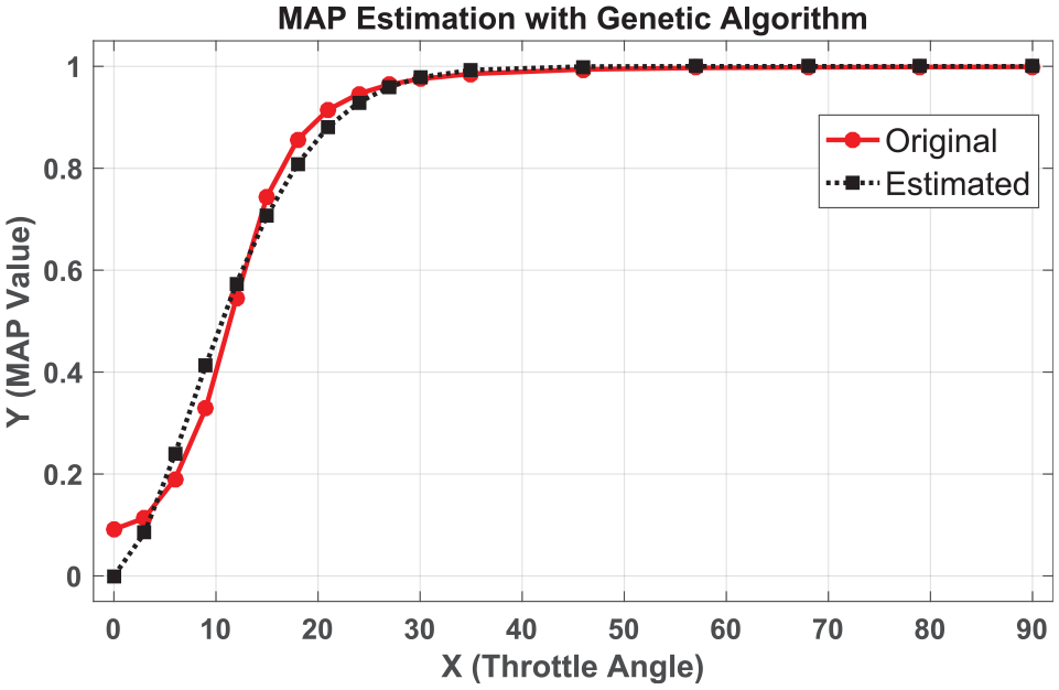
Once the fitness function is minimized and the optimum values of unknown coefficients are found, the estimated values are found by using MATLAB. The relation between original and estimated values is elaborated by the line fit plot as given below in Figure 8.
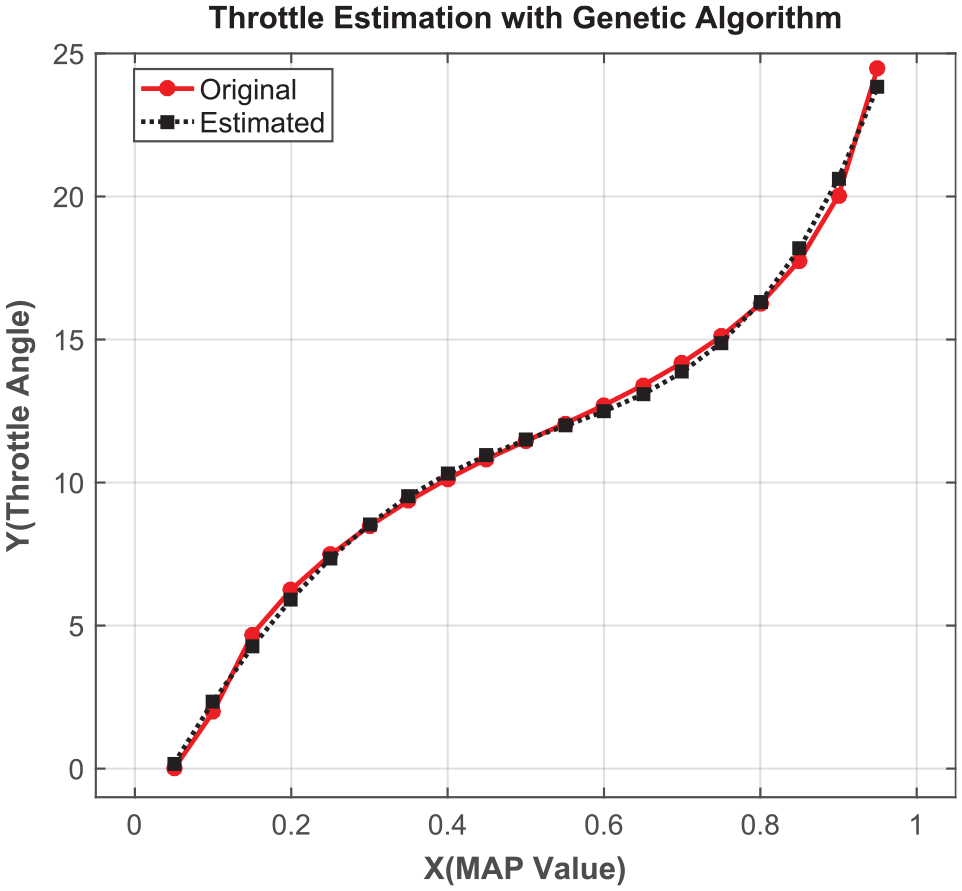
Line fit plot for original and estimated throttle sensor values.
In Figure 8 the R2 is equal to 0.997 and we can notice that the estimated values are very close to the original values which proves the efficiency of GA for the estimation of Throttle values. It can also be noticed from Figure 7 that the number of unknowns was 5 for throttle estimation so it took GA a little bit longer to reach the optimum solution. GA reached its optimum solution in 192 generations as compared to 42 for MAP estimation.
MATLAB simulation results
The proposed AFTCS for the AFR controller was implemented in MATLAB/Simulink in which GA estimation results obtained in section 3.1 were used to construct the observer model in the FDI unit. The FIU injects the fault into each sensor one at a time, leaving the others in a healthy state. In standard conditions, the mixture AFR ratio is held at 14.6, but in defective conditions, it drops to 11.7 (rich mixture). The system, however, retains reliability despite decay, which is consistent with AFTCS’s architecture philosophy.
The AFTCS part is simulated with faults in the sensors taking one sensor at a time and the effects on the AFR are observed at t = 5 s due to internal warm-up delay incorporated in the model. Figure 9 depicts the performance of the proposed AFTCS under both normal and faulty situations.
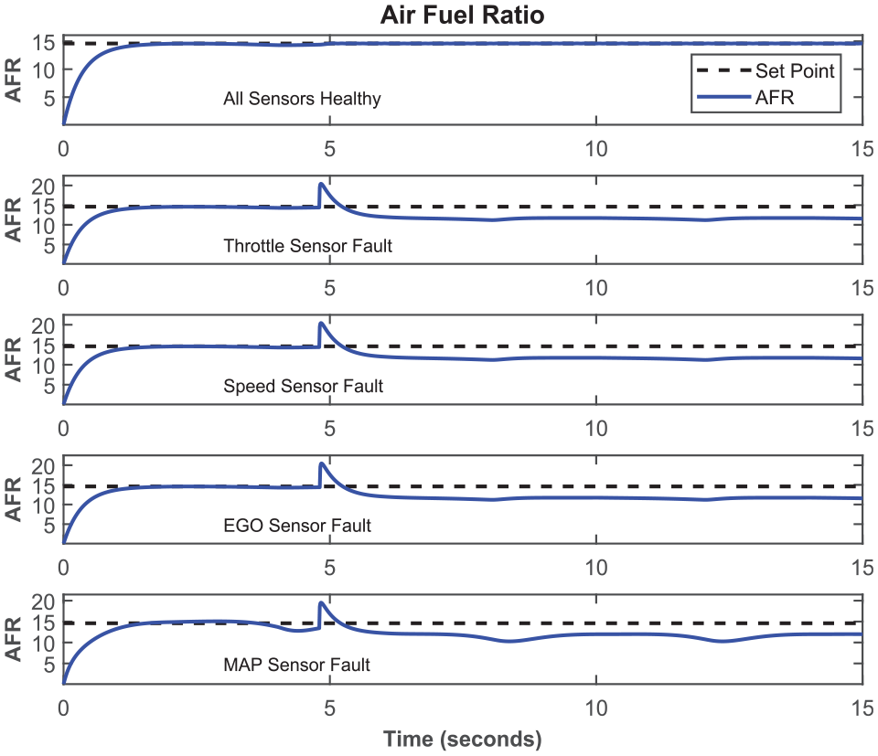
AFTCS performance for AFR control of IC engine.
Results of Figure 9 show that the AFR gets degraded to 11.7 in the steady-state with the fault in any one sensor with the AFTCS part alone. The slightly different transient behavior with the MAP sensor fault is caused by the MAP value at a throttle angle of 0°. The approximate output value obtained from the GA estimation block is slightly different from the actual value, hence it is causing a negligible oscillatory response.
Comparison with existing techniques
In this section, a comparison of the proposed GA-based AFTCS has been carried out with other existing techniques found in the literature. First, we have presented a detailed comparison for the MAP and throttle sensor estimation results with paper. 11 Afterward, we have also given a comparison with some other similar papers to show the superior performance of the proposed control system.
MAP sensor
To back up the point of improved accuracy, the same data is subjected to linear regression and MAP values are calculated. Line fit plots, as shown in Figure 10, show a comparison of predicted MAP values for GA-based estimation and linear regression.
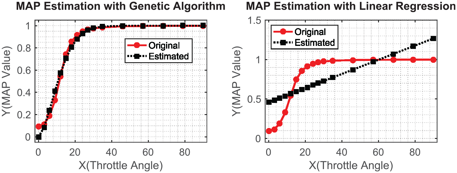
MAP estimation comparison with GA and linear regression.
We can notice from Figure 10 that linear regression is poorly estimating the sensor values. On the other hand, the GA estimated values are very close to the original values of the sensor in the nonlinear range. Table 3 shows the estimation statistics for both GA and linear regressions to demonstrate it mathematically.
Estimation statistics for MAP sensor.
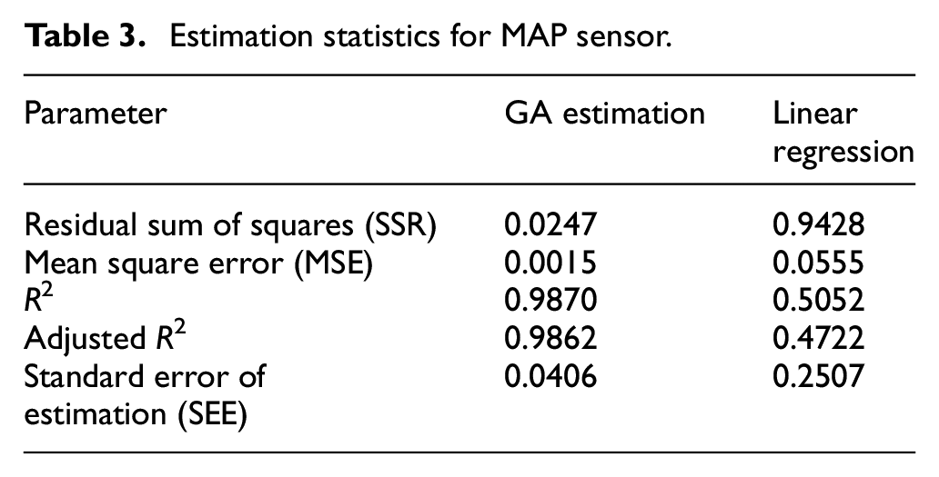
Table 3 demonstrates GA estimation’s superior efficiency, as the adjusted R2 and R2 values for GA estimation are much higher than their linear regression counterparts. In linear regression, the adjusted R2 is 0.4722 which is an indicator of poor performance of linear regression. Only R2 or adjusted R2 values are insufficient for comparison in estimation problems, so we computed the standard error of estimation, which is the best measure of estimation accuracy. Table 3 shows that the SEE in GA estimation is 0.0406 while it is 0.2507 in linear regression. An 83.5053% increase in SEE is indicating that GA estimation produces more reliable results.
Throttle sensor
To back up the point of improved precision, the same data is subjected to linear regression, and throttle angles are calculated. The line fit plots for both GA and linear regressions, as shown in Figure 11, provide a comparison of approximate throttle angles for GA and linear regression.
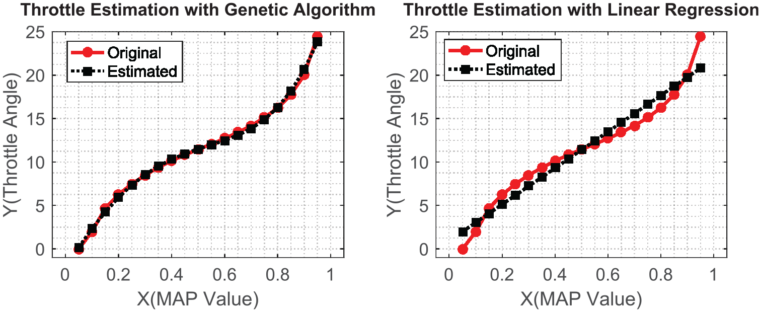
Throttle estimation comparison with GA and linear regression.
The line fit plots show that GA estimation is more reliable than linear regression in generating accurate results. Table 4 shows the estimation statistics for both GA and linear regressions to demonstrate it mathematically.
Estimation statistics for throttle sensor.
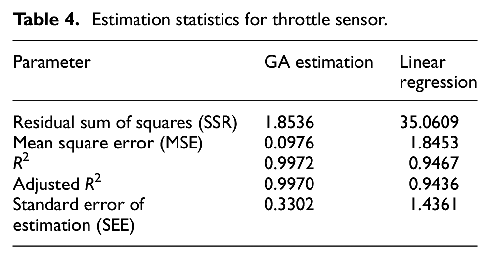
The standard error of the estimate is calculated along with other estimation statistics, just as in MAP estimation. The SEE in GA estimation is 0.3302, while the SEE in linear regression is 1.4361, demonstrating the superior output of GA estimation and a 77.0071% improvement in SEE. Similarly, for GA estimation, the adjusted R2 and R2 values are superior to their linear regression counterparts.
Apart from linear regression-based observer design, the existing models used lookup tables, KF, and ANN for the fault-tolerant AFR system design. Lookup tables and ANN techniques are computationally less efficient and KF is limited to the linear region of the sensors. Some other techniques are also using some advanced algorithms like SVM, deep learning, CVA, or EWMA. But in these advanced techniques, we need a large dataset. Our contribution to this research is the implementation of a GA-based observer model in the FDI unit. The proposed method is producing excellent results (up to 77% improvement in the standard error of estimation) despite having a limited dataset. The proposed method uses GA which tends to find the local optimum solution and can be used on the hardware with limited computational power or in time-critical applications. In comparison to previous literature works, the simulation results show superior fault tolerance efficiency, particularly for the MAP sensor, in terms of less oscillatory response.
Complexity analysis
One of the objectives of this study was to design a fault estimation technique for time-critical systems and devices with memory or processing constraints of the commercially available controllers. For this purpose, a simple GA was used to estimate the sensor values in faulty conditions. The other possible choices for the estimation may be PSO, ANN, or any other advanced optimization algorithm. PSO tends to find the global optimum solution due to which the computational complexity of PSO is large, and the pace of convergence is sluggish. Its high computational complexity makes it unsuitable for low-power applications, 49 while its slow convergence speed makes it unsuitable for time-critical applications. On the other hand, GA used in this study is finding the local optimum solution due to its discrete nature hance the GA will be computationally effective in this case. The tendency of premature convergence in PSO is also high as compared to GA. 50 Forward propagation and backpropagation are the two main processes in ANN training and the complexities of these operations are of fifth-degree polynomial. Moreover, the backward propagation has the property of low convergence rate and weak generalization capacity 51 which makes it computationally inefficient. Therefore, for an optimization problem, the computational complexity depends upon the problem itself instead of the algorithm. And the estimation problem considered in this study is having a limited dataset and is of moderate complexity, hence GA would be a suitable option in this case.
Conclusion
In this paper, an improved AFTCS for the AFR control system of an IC engine was proposed to improve reliability and avoid expensive shutdowns due to sensor failures. The FDI unit in the proposed AFTCS was developed using a genetic algorithm-based observer unit. The model was checked for different sensor faults in the MATLAB/Simulink environment. The proposed model produced excellent results (up to 77% improvement in the standard error of estimation) despite having a limited dataset. The proposed method used GA which tends to find the local optimum solution and can be used on the hardware with limited computational power or in time-critical applications. In comparison to previous literature works, the simulation results showed superior fault tolerance efficiency, particularly for the MAP sensor, in terms of less oscillatory response.
Since we used full-type sensor faults as a limiting case of testing, future studies could use the AFTCS architecture for partial-type sensor faults with the hardware-in-loop-verification of the proposed algorithm. Another direction could be considering non-fragile control to deal with the various disturbances in a practical scenario.
Footnotes
Declaration of conflicting interests
The author(s) declared no potential conflicts of interest with respect to the research, authorship, and/or publication of this article.
Funding
The author(s) received no financial support for the research, authorship, and/or publication of this article.