Sage Journals: Discover world-class research

Abstract

The probability of electric vehicle rollover accident can be effectively reduced by shortening the prediction time interval and improving the prediction accuracy. Based on a multilayer neural network, an improved time-to-rollover method is presented in this paper. Firstly, the force model of vehicle rollover is established and analyzed where the structure and mass of a battery box have an important influence on the occurrence of rollover. Then, the rollover indexes considering hyperparameters are divided into five categories, and the multi-layer neural network is used to simplify the algorithm structure of the time to rollover, and quickly calculate the operating state parameters with a variation step size in real time. Finally, the influence of the hyperparameters on the prediction results of neural network is studied, and higher efficiency is obtained by comparing with traditional methods.

Keywords

New energy vehicle rollover model neural network time-to-rollover

Introduction

New energy vehicles have become a hot direction of scientific research in recent years.¹ It is necessary to develop an effective rollover warning model to reduce the probability of rollover due to emergency avoidance of obstacles during high-speed driving.^2,3

Chen^4–6 proposed firstly a time to rollover (TTR) considering the vehicle rollover of a three-degree-of-freedom to study rollover time. The TTR owns simple and real-time, which makes it easy to transplant to rollover alarm controller. Later, a vehicle rollover warning algorithm was used by Zong et al.⁷ for heavy commercial vehicle based on prediction model. Through combing the merits of angle and angular acceleration, a dual-axis rollover model with the integrated combination angle stiffness of suspension and tire vertical stiffness was established Wei et al.⁸ to study a warning algorithm of bus rollover based on roll angle threshold. Rajamani et al.⁹ investigated a sensor fusion algorithm with the combination of a gyroscope for real-time rollover estimation. Dynamics analyses of a 5-degree-of-freedom model and an 8-degree-of-freedom model were compared by Yu et al.¹⁰ for a heavy semi-trailer. However, the above methods based on the TTR only considered the one-to-one relationship between input and output, which significantly increased the computational cost and complicated the algorithm structure, because the TTR needed to calculate the operating state parameters of the vehicle in real time.^11,12

In recent years, the artificial neural network has been applied in many fields, including intelligent video surveillance, automatic driving, and motion recognition.^13–15 Additionally, many remarkable achievements have been made in topology optimization of material structure, effective performance prediction, and multi-scale composite design using the artificial neural network.^16,17 Flight parameters were used by Belge et al.,¹⁸ to plan and track the path with minimum energy and time consumption for unmanned aerial vehicle. Additionally, the neural network based real-time control of a hexarotor unmanned aerial vehicle was performed by the same authors to reduce error for payloads on the targets determined by path tracking.¹⁹ This is because the artificial neural network can find and analyze high-dimensional approximate functions through a large number of inputs.²⁰ Rao and Liu²¹ studied three-dimensional convolutional neural network for heterogeneous material homogenization. Effect of constituent materials on composite performance was explained by Chen and Gu²² by exploring design strategies via machine learning. Utilizing a neural network, Chen and Peng²³ took the TTR generated by the simple model, roll angle, and change of roll angle to generate an enhanced NN-TTR index which can boost the performance of simple TTR algorithm effectively. By employing neural network method, Treetipsounthorn and Phanomchoeng²⁴ developed a rollover algorithm to prevent tripped rollovers from external inputs such as tripping by the force of a vehicle striking a curb or a road bump. To ameliorate the deficiency of rollover indicators in existing warning models, Dong et al.²⁵ proposed an improved rollover index based on BP neural network, taking the road inclination angle, the steering strategy, and the hydropneumatic suspension characteristics into consideration. A novel rollover prevention control system composed of rollover warning and integrated chassis control algorithm was developed by Zhu et al.²⁶ using a back-propagation neural network. The results showed that the presented algorithm can be a good measure of the danger of rollover. A superior vehicle rollover warning algorithm was proposed by Zhu et al.²⁷ considering the nonlinear characteristic of driver-vehicle-road interaction and uncertainty of modeling. The novel algorithm provided an explicit function of vehicle rollover safety limit and its gradient, and defined the rollover safety area and the unsafe area through the hypersurface visualization boundary. In above references, the TTR method uses a fixed step size to detect the rollover index in real time, make a judgment on whether the threshold value is reached and decide whether to issue a warning.²⁸ However, the fixed step size may result in wasted time when the vehicle is in a low-risk condition. Additionally, the power battery box often occupies a large part of the space of the vehicle as the main source of energy for the vehicle; then, it is important to consider the structural arrangement and mass of the battery box of the new energy vehicle to analyze whether the whole vehicle is overturned. Then, an improved TTR new energy vehicle warning algorithm based on multilayer neural network is proposed. Compared with the traditional TTR method, the advantages of the presented warning model are the following: (1) By training a multilayer neural network to simplify the algorithm structure of the TTR and quickly calculate the operating state parameters in real time, various rollover influencing factors can be considered simultaneously as inputs to predict the results of rollover indicators and reduce the computational cost. (2) Since the structure and mass of the battery box have an important influence on the occurrence of rollover in new energy vehicles, the influence of the ratio of the height of the battery mass center to the height of the whole vehicle mass center and the weight of the battery box on the rollover index is focused on. (3) The rollover indexes are divided into five categories to more comprehensively evaluate the rollover results. (4) Based on the predicted categories of rollover indexes, variable steps are selected to calculate the rollover time TTR.²⁹

The rest of this paper is organized as follows: A 3-degree-of-freedom new energy vehicle rollover model is established, in which suitable rollover warning indexes are considered; additionally, based on multilayer neural network, an improved TTR algorithm is given in Section 2. Then, the effect of several neural network hyperparameters on the prediction of the rollover index is analyzed. Furthermore, the results of the traditional TTR algorithm are compared with the presented TTR algorithm in Section 3. Finally, the conclusions are given in Section 4.

Establishment of model and character recognition

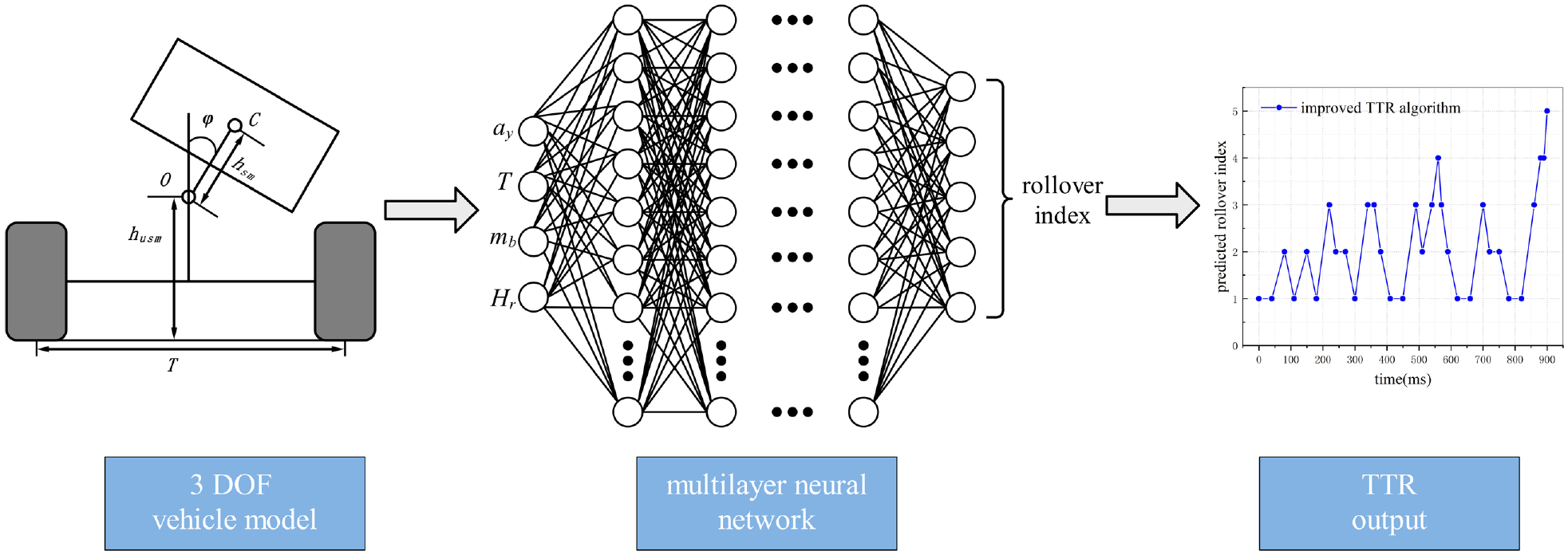
The flow of the improved TTR warning algorithm applying multilayer neural network is shown in Figure 1.

Figure 1.

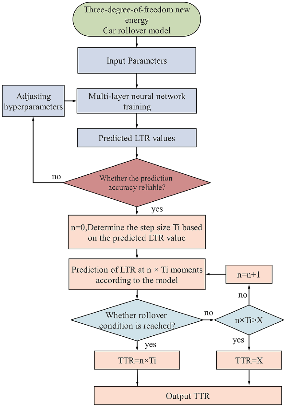
Improved TTR warning algorithm process with application of neural networks.

A 3-degree-of-freedom new energy vehicle rollover model is established, and the crucial influencing parameters on rollover are determined by dynamics analysis as the input for neural network training. The lateral load transfer rate (LTR) was selected as the output of the neural network to represent the risk of rollover. The results are classified into five categories, with higher LTR values indicating a higher risk of rollover. The prediction accuracy is evaluated, if it does not meet the requirements, the neural network structure needs to be adjusted and the above steps are repeated until the results meet the standards. Set the time threshold X to calculate the rollover result within one period X. Different Ti values are selected to calculate the TTR time based on the predicted LTR results. Keep repeating the process of neural network training – predicting LTR – accumulating Ti values until a certain result reaches the rollover index, the loop is terminated and output the TTR rollover time. In addition, if the rollover condition is not reached in one period X, the TTR time is also output and goes to the next cycle of warning detection.

Three-degree-of-freedom car model

A three-degree-of-freedom car rollover model is established as shown in Figure 2, and the D’Alembert principle is applied to convert the rollover dynamics problem into a hydrostatic equilibrium problem. It is easy to know by analysis that the forces in the vertical axis direction and horizontal axis direction are balanced. List the moment balance hydrostatic equations on the axes, establish a simple model, and analyze the main factors affecting the vehicle rollover and rollover stability.²⁷

Figure 2.

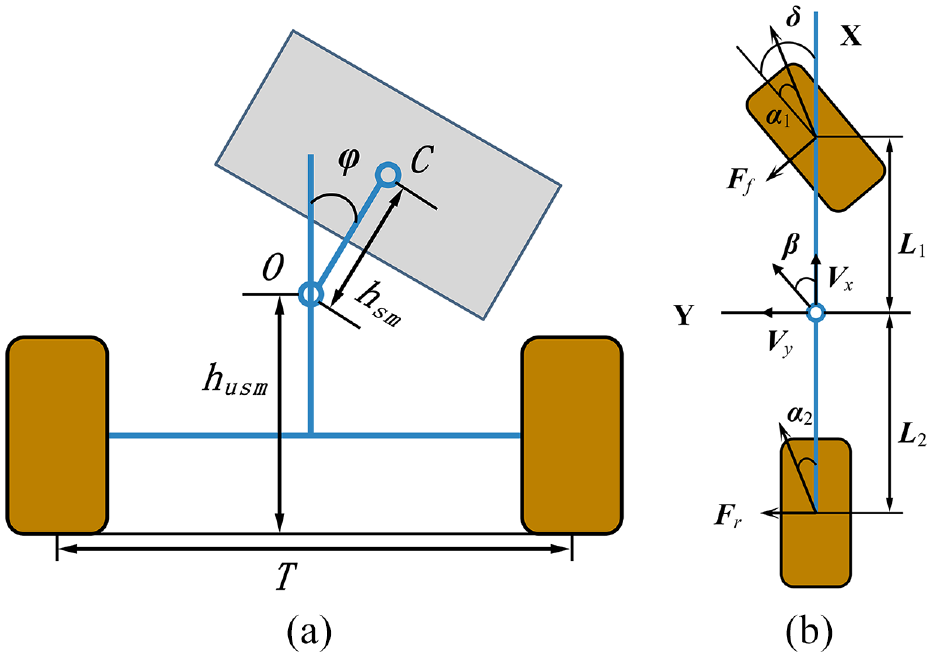
Three-degree-of-freedom vehicle rollover reference model: (a) schematic diagram of the lateral tilt plane and (b) schematic diagram of the same-side wheels.

It should be noted that, in order to accurately study the stability of vehicle rollover, it is necessary to establish an ideal rollover model that reflects the rollover pattern of the vehicle. For the convenience of calculation, often ignoring some minor elements, the following assumptions need to be made in the establishment of this model.^29,30

Assume that the longitudinal velocity of the vehicle’s center of mass is constant.

The vertical motion of the vehicle is not considered.

Assuming that the vehicle travels on an ideal horizontal surface.

No consideration of aerodynamic effects.

Neglecting the effects of the nonlinear characteristics of the suspension, and the asymmetry of the front and rear axles.

Neglecting the effects on the tire characteristics due to the return torque of the tires and the variation of the left and right wheel loads.

In Figure 2: $C$ is the center of mass of the whole vehicle part, $O$ is the center of mass of the battery box, $h_{usm}$ is the height of the center of mass of the battery box to the ground, $h_{sm}$ is the distance from the center of mass of the whole vehicle to the center of mass of the battery box, $ϕ$ is the rollover angle, $v_{x}$ is the longitudinal velocity, $v_{y}$ is the lateral velocity, $δ$ is the front wheel steering angle, $β$ is the mass lateral deflection angle, $L_{1}$ is the distance from the center of mass to the front axle, $L_{2}$ is the distance from the center of mass to the rear axle, $α_{1}$ is the lateral deflection angle of the front wheel, $α_{2}$ is the lateral deflection angle of the rear wheel, $F_{f}$ is the lateral deflection force from the ground to the front wheel, and $F_{r}$ is the lateral deflection force from the ground to the rear wheel.

The basic kinetic equation of the car can be listed as³¹:

a_{y} = {\overset{\cdot}{v}}_{y} + v_{x} ω

(1)

β = \frac{v_{y}}{v_{x}}

(2)

F_{f} = k_{1} α_{1} = k_{1} (β + \frac{L_{1} ω}{v_{x}} - δ)

(3)

F_{r} = k_{2} α_{2} = k_{2} (β - \frac{L_{2} ω}{v_{x}})

(4)

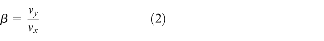
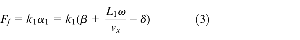
where $a_{y}$ is the lateral acceleration; $ω$ is the angular velocity of the transverse pendulum; $k_{1}$ is the equivalent lateral deflection stiffness of the front wheel; $k_{2}$ is the equivalent lateral deflection stiffness of the rear wheel.

Take moments for the point $O$ of the vehicle model in Figure 2, applying D’Alembert’s principle, the equilibrium equation can be obtained as:

I_{ZZ} \overset{\cdot}{ω} = L_{1} F_{f} \cos δ - L_{2} F_{r}

(5)

m a_{y} - m_{b} h_{sm} \overset{\cdot\cdot}{ϕ} = F_{f} + F_{r}

(6)

where $m$ is the mass of the whole vehicle, $m_{b}$ is the mass of the battery box part, $I_{ZZ}$ is the vertical rotational inertia.

To reduce the measurement difficulty, the initial $\overset{\cdot}{ω}$ and ${\overset{\cdot}{v}}_{y}$ are assumed to be zero here, while ignoring the nonlinearities of the suspension and the effect of different characteristics of the front and rear axles on the warning algorithm.

The important physical quantity, the angular velocity of the pendulum $ω$ , can be obtained after the derivation of the known quantity, the steering wheel angle $δ$ , by substituting the equations (1)–(6).

The kinetic equation is calculated by analyzing the spring-loaded part of the car separately and taking the moment for the center of mass point.

K ϕ + I_{XX} \overset{\cdot\cdot}{ϕ} - m_{b} a_{y} h_{sm} \cos ϕ - m_{b} g h_{sm} \sin ϕ = 0

(7)

Suppose that $\overset{\cdot\cdot}{ϕ} = 0$ , then we have:

h_{sm} = K ϕ / (m_{b} v_{x} ω \cos ϕ + m_{b} g \sin ϕ)

(8)

where $K$ is the suspension equivalent damping factor; $I_{XX}$ is the longitudinal rotational inertia.

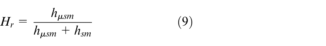
The battery center of mass height to vehicle center of mass height ratio into consideration, which can be expressed as $H_{r}$ :

H_{r} = \frac{h_{μ sm}}{h_{μ sm} + h_{sm}}

(9)

Previously, it has been derived from the steering wheel angle $δ$ expressed by $ω$ , the rollover angle $ϕ$ can be measured by the sensor, and the height of the spring loaded $h_{sm}$ is derived from equation (8), and the height of the center of mass of the whole car $H_{r}$ is derived from equation (9). Considering that when the car occurs at low speed stable steering, there is a stable rollover angle, so the automatic calculation of the center of mass height need to meet the car low speed stable steering conditions. Due to the low-speed steady steering condition and the weakness of the hysteresis, the measured value of the roll angle sensor can be used in the calculation of the center of mass height.

\begin{matrix} m a_{y max} H_{r} (h_{μ sm} + h_{sm}) (1 + \frac{h_{sm}}{h_{μ sm}} \cos ϕ) \\ = mg (\frac{T}{2} - h_{sm} ϕ_{max}) \end{matrix}

(10)

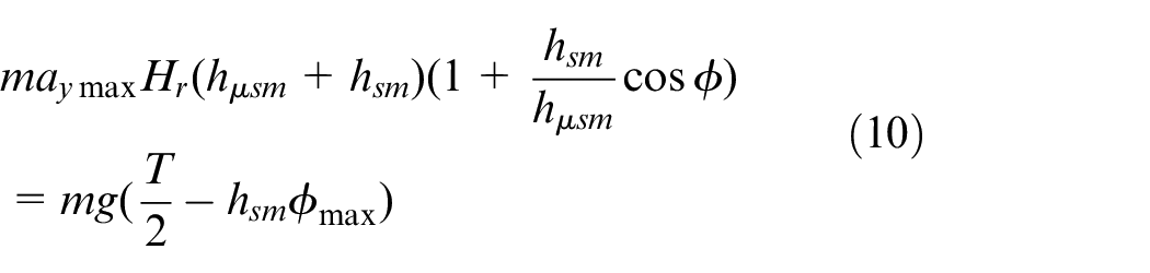
The inside wheel vertical load is zero if the car reaches the critical state of rollover. Additionally, the rollover angle in equation (8) is set to the maximum value $ϕ_{max}$ , and the lateral acceleration $a_{y max}$ can be calculated by associating equation (10).

Selection of rollover warning index

The selection of rollover indexes directly affects the accuracy of the vehicle rollover warning system. The rollover indexes are usually selected from parameters affecting vehicle rollover factors such as lateral acceleration, rollover angle, vehicle center of mass position, rollover energy value, and tire vertical load, among which lateral acceleration and rollover angle are the most commonly used rollover indexes. However, due to the motion state before the vehicle rollover is often very violent, and the rollover thresholds of different vehicle models and vehicle driving conditions are very different, there are limitations in using the above parameters as rollover indexes.

Firstly, the relative quantity of the ratio of the current lateral acceleration of the vehicle to the real-time lateral limit acceleration is discussed as a rollover determination condition to evaluate the dynamic process of the traveling vehicle. Compared with the traditional evaluation index, the selection method of the rollover threshold for this evaluation index is relatively simple. When the ratio exceeds 1, it means that the current lateral acceleration of the vehicle exceeds its limit value and rollover is about to occur. Further, by analyzing the dynamic balance of the vehicle in the lateral tilt direction, the lateral limit acceleration of the vehicle can be obtained in real time, and then the ratio of the lateral acceleration to the real-time lateral limit acceleration is calculated, and the ratio and the TTR method are integrated to calculate the time limit value of the vehicle when the rollover occurs in the future.

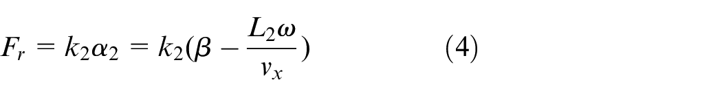
Additionally, the steering wheel turning angle can be chosen as the threshold of rollover warning and the input of neural network training. Selecting the steering wheel turning angle as the warning indicator can effectively improve the problem that the results of the existing TTR rollover warning algorithm lag behind the actual motion state of the vehicle. By analyzing the established mathematical-physical model of the vehicle, the factors that may have an impact on vehicle rollover, such as the lateral camber angle, lateral acceleration and vertical load, are represented by the steering wheel rotation angle and vehicle speed. The kinetic relationship between the above influencing factors and the steering wheel turning angle is further derived, and the TTR based on the steering wheel turning angle is derived using the steering wheel turning angle as the rollover threshold, so as to achieve the purpose of predicting the rollover risk earlier.

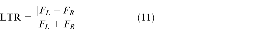
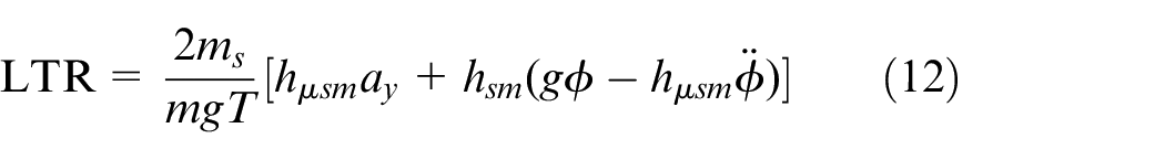
The lateral load transfer rate (LTR) is selected as the vehicle rollover warning parameter in this work. LTR is defined as the ratio of the absolute value of the difference between the left and right wheel vertical loads to the sum of the left and right wheel vertical loads, which is defined as follows.

LTR = \frac{| F_{L} - F_{R} |}{F_{L} + F_{R}}

(11)

where $F_{R}$ denotes the right wheel vertical reaction force and $F_{L}$ denotes the left wheel vertical reaction force.

When the vehicle is safely driven on a good road surface with equal vertical loads on the left and right wheels, LTR = 0; When the vehicle rolls over under extreme working conditions, one of the wheels of the vehicle leaves the ground, LTR = 1. Meanwhile, LTR, as a rollover indicator, is a dimensionless parameter, independent of vehicle type or speed, having good generalizability. We classify the results of LTR into five categories. 0 ≤LTR < 0.2 will be recorded as 1; 0.2 ≤ LTR < 0.4 will be recorded as 2; 0.4 ≤ LTR < 0.6 will be recorded as 3; 0.6 ≤LTR < 0.8 will be recorded as 4; 0.8 ≤LTR ≤ 1 will be recorded as 5. The smaller the rollover indicator means the smaller the risk of rollover, when LTR = 1 means one side of the wheel has left the when LTR = 1, it means that one side of the wheel has left the ground.

Considering that the vertical loads on both sides of the wheels change in real time and are not easily measured while the car is moving, it is difficult to calculate the LTR value directly by equation (11). Therefore, by substituting equation (11) of the definition of LTR into the model for linear transformation, we can obtain that:

LTR = \frac{2 m_{s}}{mgT} [h_{μ sm} a_{y} + h_{sm} (g ϕ - h_{μ sm} \overset{\cdot\cdot}{ϕ})]

(12)

The traditional TTR rollover warning algorithm reflects the vehicle rollover risk by predicting the rollover time TTR in real time. The TTR is defined as the time required from the current moment to the moment when one wheel leaves the ground, and the ideal TTR curve is a straight line with a slope of one.

The TTR-based rollover warning algorithm is based on the rollover indicator LTR to determine the input of the model and calculate the LTR value in the current state by the established rollover model. A fixed step $G$ is chosen, and the LTR value at the future time is calculated by $n \times G$ . While compared with the LTR threshold, if the rollover condition is not yet reached then the next iteration process is entered as $n = n + 1$ . Assuming that the number of steps to reach the rollover condition is N, the warning time is $TTR = N \times G$ , which means the vehicle will roll over and trigger the active rollover prevention system within the $N \times G$ time. The warning time threshold $X$ is also set to ensure the timeliness of the warning model, and if the rollover condition is not reached within the time $X$ , the warning will be calculated in the next iteration.

Improved TTR method

Part A provides the kinetic analysis of the new energy vehicle rollover, after which, lateral acceleration $a_{y}$ , wheelbase $T$ , battery center of mass height to vehicle center of mass height ratio $H_{r}$ and battery box weight $m_{b}$ are selected as inputs, and lateral load transfer rate (LTR) is taken as the vehicle rollover early rollover warning index which is the output of multilayer neural network. The result of LTR is divided into five categories which smaller rollover index means the smaller the risk of rollover, and when LTR = 1, it means that one side of the wheel has left the ground. Depending on the output results, different intervals are taken for the next rollover index prediction. These time intervals are recorded and accumulated to obtain the TTR time within a cycle eventually. The complete structure of the improved TTR algorithm is demonstrated schematically in Figure 3.

Figure 3.

Architecture of improved TTR algorithm.

For the difference under the traditional TTR rollover warning model, the neural network is used for train the relationship between rollover-related influencing factors and rollover indicators. Additionally, the multiple influencing factors are considered as input values for the model at the same time. Then, the influence of battery box parameters is considered on the rollover phenomenon of new energy vehicles, in which the more comprehensively assess are given to consider whether there is a risk of rollover occurring. The machine learning prediction method can avoid real-time calculations, further boosting the performance while reducing computational costs. In addition, the rollover indicators are divided into five categories according to the value of LTR, which can more refine the description of rollover risk and enable drivers to grasp the current driving conditions more comprehensively.

In order to better improve the performance of the algorithm, the sampling time of the vehicle acceleration sensor needs to be considered. There are various implementations of traditional acceleration sensors, which can be mainly classified as piezoelectric, capacitive, and thermal sensing, and each of these three technologies has its own advantages and disadvantages. Acceleration sensors are also characterized by different specifications for different application scenarios. Generally, the sensors used in the body of the car need to choose high frequency (50–100 Hz) acceleration sensor.

The warning time threshold X is considered as 2 s; based on the classification of the rollover indicator, the step value $T_{i}$ (i = 1,2,3,4,5) is classified for calculating the rollover time TTR, in which the step is a fixed value in the traditional TTR. The specific classification is as follows.

According to the frequency of the accelerometer above, we make the following settings: when the rollover indicator is 1, the step length $T_{1}$ = 40 ms; when the rollover indicator is 2, the step length $T_{2}$ = 30 ms; when the rollover indicator is 3, the step length $T_{3}$ = 20 ms; when the rollover indicator is 4, the step length $T_{4}$ = 10 ms; when the rollover indicator is 5, the rollover indicator is reached and the algorithm is terminated. The reasonableness of this classification is that the smaller the rollover indicator indicates the smaller the current rollover risk, then correspondingly, a larger step can be set relatively when calculating the warning indicator LTR at the moment of $n \times T_{i}$ to improve the warning efficiency. On the contrary, when the rollover indicator is larger, a smaller step can be set, because a larger rollover indicator indicates a high rollover risk, and a smaller step can achieve multiple detections in a short period of time, and warn immediately once the rollover condition is reached.

Since the large range of values and different units of the input data for multilayer neural networks, training neural networks directly may lead to an increase in the error of prediction results. Therefore, it is necessary to preprocess the data before training. The advantage of preprocessing data using normalization is that in machine learning or deep learning, the loss calculation for most models requires the assumption that all features of the data are zero-mean and have the same order of variance. This way, all feature attributes can be treated uniformly when calculating the loss.

Normalization of data is the scaling of data so that it falls into a small specific interval. It is often used in certain comparisons and evaluations of metrics to remove the unit constraints of the data and transform them into dimensionless pure values, so that metrics of different units or magnitudes can be compared and weighted. The most typical of these is the normalization of the data, that is, mapping the data uniformly to the [0,1] interval (or the desired interval).

There are different normalization methods for different problems. The common normalization methods are as follows: (1) Linear normalization; (2) Polar difference transformation method; (3) Mean value normalization; (4) Nonlinear normalization. Nonlinear normalization refers to the mapping of the original values by some mathematical functions (log, tan, exp, and other functions) that distribute the data into the desired range.

In this work, considering the computational cost and the impact of various normalizations on the model results, we use the polar difference transformation method to pre-process the data. There are four inputs to the multilayer neural network, namely, lateral acceleration, wheelbase, battery mass center height to whole vehicle mass center height ratio and battery box weight, with a total of 1500 data for each input.

Numerical examples and discussion

Effect of the number of hidden layers on prediction accuracy

In the application of machine learning methods, the selection and debugging of hyperparameters in multilayer neural networks have a huge impact on the results, and the results obtained by using different hyperparameters vary widely, sometimes by a thousandth of a percent, with worlds of difference. For the selection of hyperparameters, there will be a general range based on experience and related literature, but a large number of tuning experiments are required to obtain the values with the best results. In the following, we will explore the effect of using different number of neurons, number of epochs, batch size, and learning rate on the prediction accuracy of multilayer neural networks, and analyze the reasons for this effect. It should be noted that the results in each section below are obtained after the program has been run at least three times, so that can effectively avoid errors caused by chance.

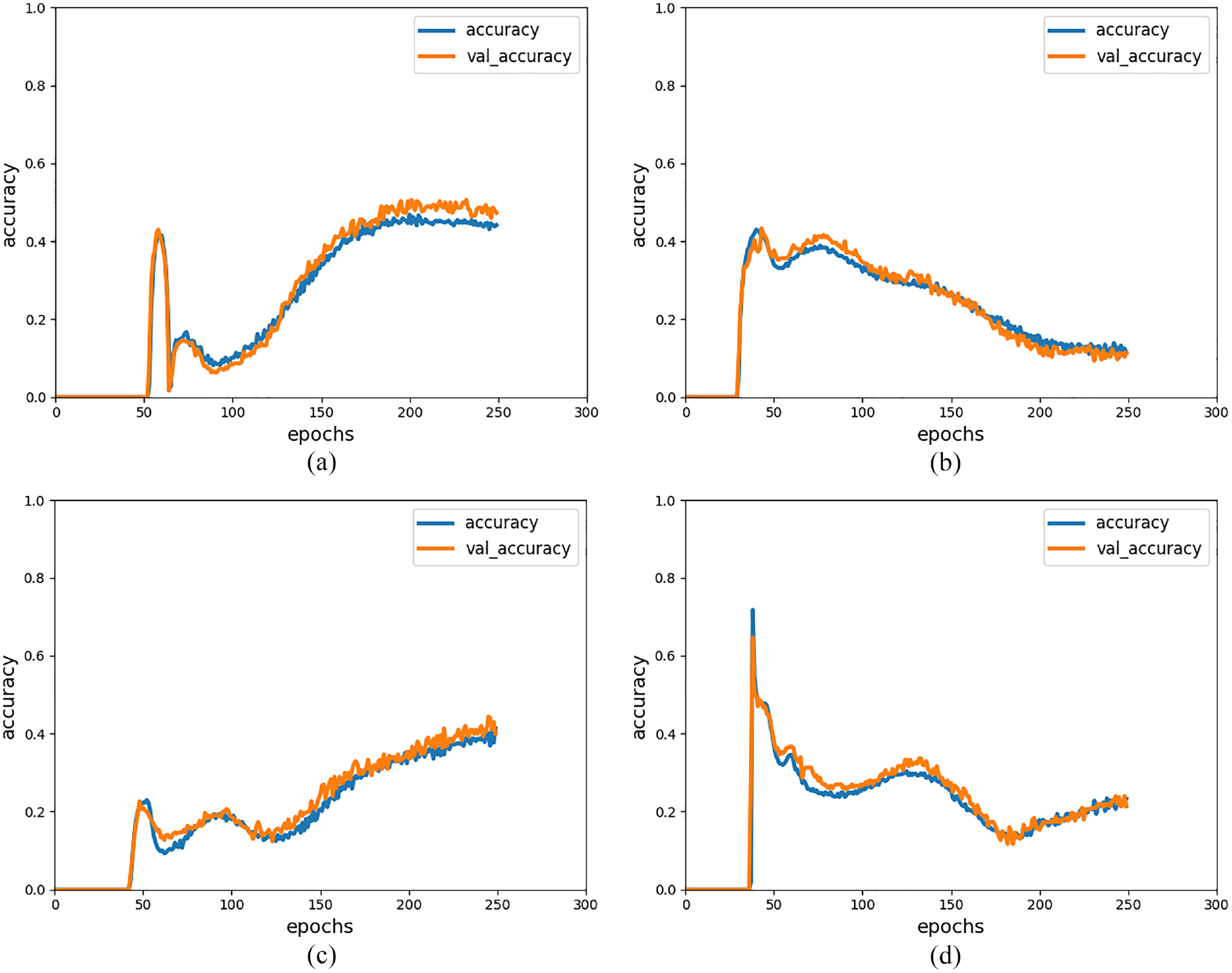
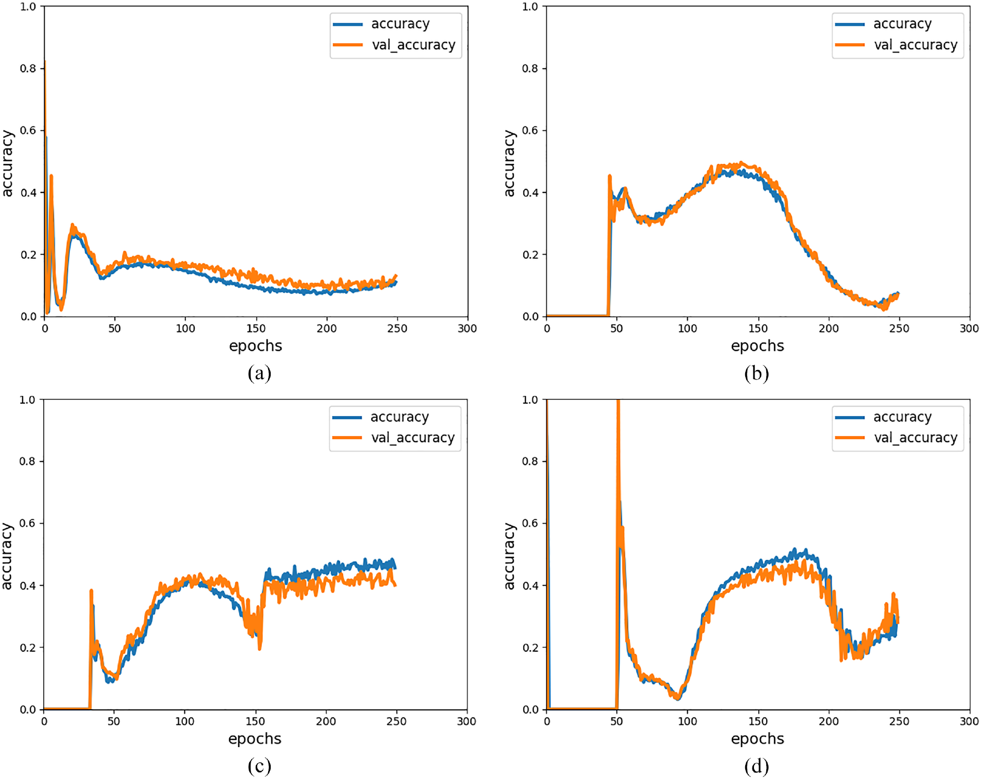
As shown in Figure 4, first we explored the relationship between different hidden layers of the neural network and the prediction accuracy. Under the conditions of batch size of 25, learning rate of 0.009, and number of epochs of 250, the results are shown in Figure 4(a)–(d) for the number of $hidden layer = 1$ , $hidden layer = 2$ , $hidden layer = 3$ , and $hidden layer = 5$ , respectively.

Figure 4.

Effect of different hidden layers on the accuracy rate: (a) one hidden layer, (b) two hidden layers, (c) three hidden layers, and (d) five hidden layers.

As can be seen from Figure 4(a), when there is only one layer of hidden layers, the accuracy of the neural network has not yet reached 0.2 at the end of the train. One possible reason is that the single-layer structure is too simple to accomplish the update of weights and bias within the network architecture. The instability in Figure 4(b) and (d) lies in the fact that there is a distinct decline in the prediction accuracy after reaching a peak, of which Figure 4(b) is particularly serious, and the accuracy has dropped to below 0.1 before the end of training. The drop in Figure 4(d) may be due to the excessive number of layers and thus the occurrence of overfitting. In contrast, the results in Figure 4(c) show that when the hidden layer is three layers, the prediction accuracy of the results finally tends to be stable as the number of training cycles on the neural network increases, and despite small fluctuations, the results are within the allowable range with better results. In summary, in the later hyperparameters debugging of the neural network, the hidden layers are all set to three layers.

Effect of number of epochs on prediction accuracy

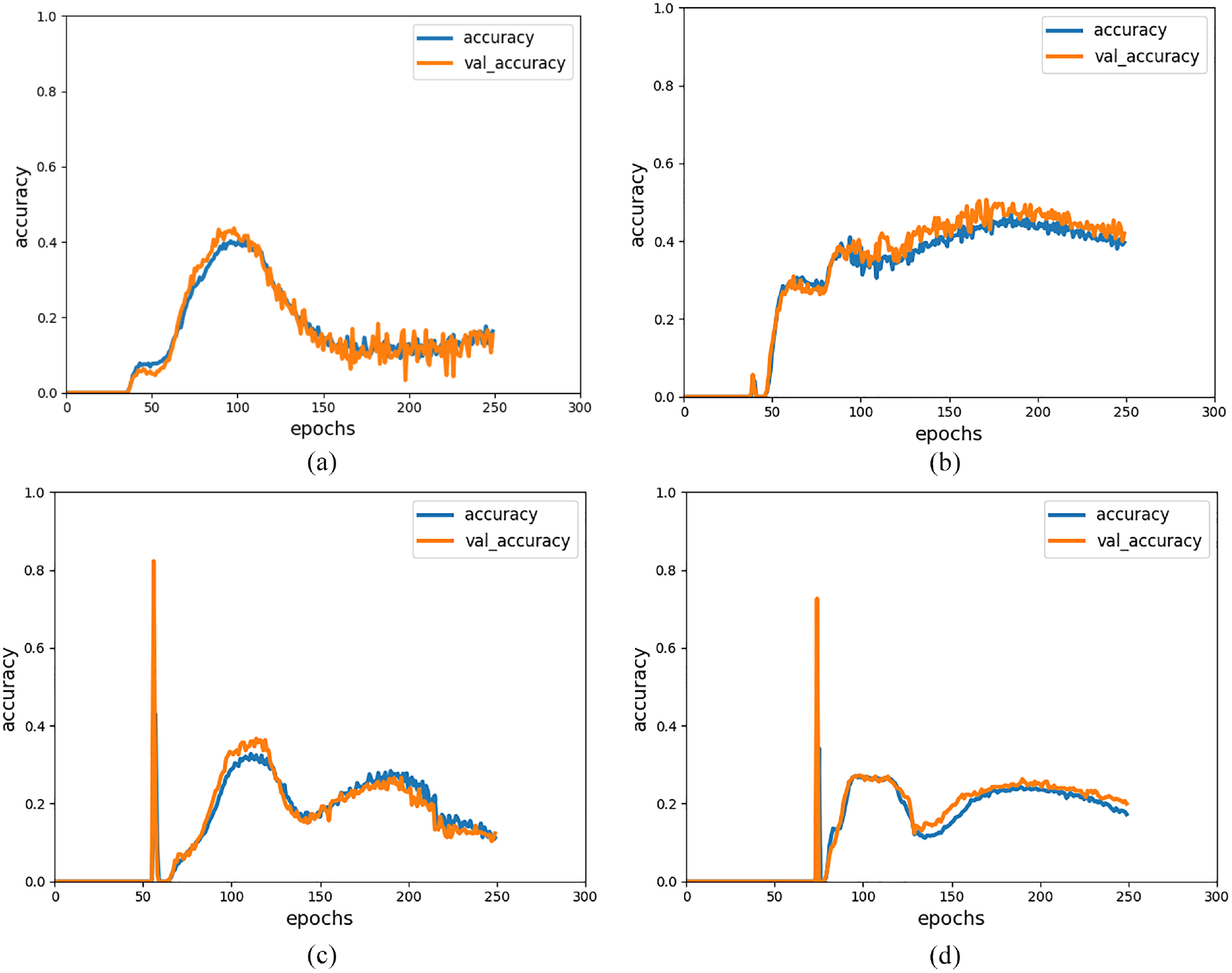
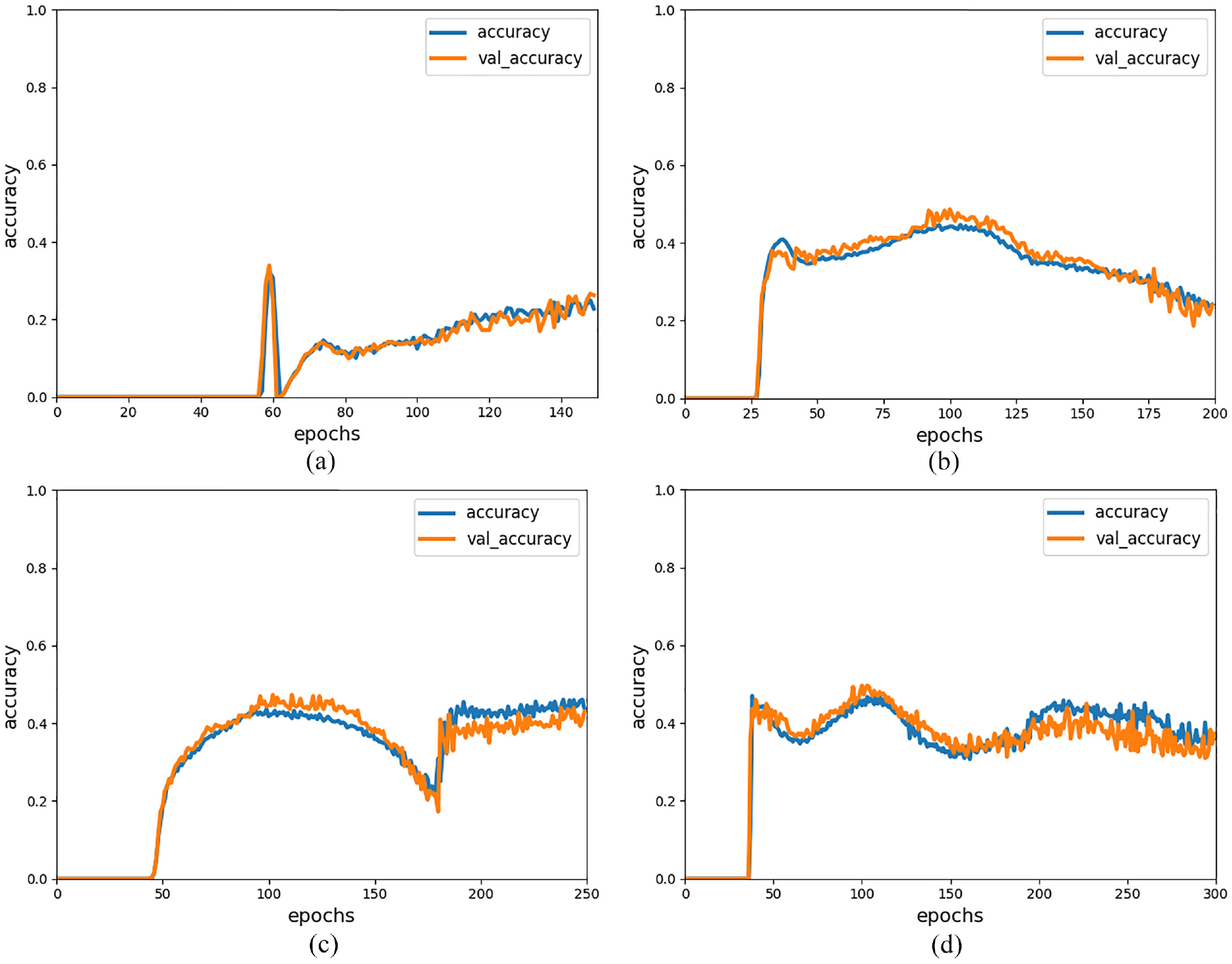
The effects of different number of cycles on the prediction accuracy are shown in Figure 5. Under the condition of batch size of 25 and learning rate of 0.009, Figure 5(a)–(d) show the results for the number of $epochs = 150$ , $epochs = 200$ , $epochs = 250$ , and $epochs = 300$ , respectively.

Figure 5.

Relationship between different number of epochs and accuracy rate: (a) epochs = 150, (b) epochs = 200, (c) epochs = 250, and (d) epochs = 300.

From Figure 5(a), the prediction accuracy is in the increasing stage but the value is only about 0.2 before the end of the training, which indicates that the number of cycles is not enough to make the neural network completely trained at this time. The whole curve in Figure 5(b) is relatively smooth, with the accuracy peaking at about 0.5, and finally trending slightly downward, basically remaining around 0.3. Compared to Figure 5(b), the curves in Figure 5(c) and (d) have different degrees of fluctuation with slightly higher peaks. In Figure 5(c) in the vicinity, there is a decreasing trend in the accuracy rate, followed by a steep increase back to 0.4–0.5, and finally stabilizes. The curve in Figure 5(d) approximates a wavy line with little overall fluctuation, and the accuracy finally stabilizes around 0.4. Comparing these four curves, we can find that the neural network can obtain better accuracy under the conditions of and the number of cycles of training of the neural network also basically reaches the threshold, and the prediction accuracy finally tends to a stable value.

Impact of learning rate on prediction accuracy

The effects of different learning rates on the prediction accuracy are shown in Figure 6. Under the condition that the batch size of 25 and the number of epochs is 250, Figure 6(a)–(d) show the results of $lr = 0.005$ , $lr = 0.007$ , $lr = 0.009$ , and $lr = 0.011$ , respectively.

Figure 6.

Effect of different learning rates on the accuracy rate: (a) lr = 0.005, (b) lr = 0.007, (c) lr = 0.009, and (d) lr = 0.011.

As can be seen from Figure 6(a), the accuracy curve has a sharp convexity around epochs of 50 and then gradually increases. Due to the small learning rate, the network needs more cycles to reach the optimal state. Figure 6(c) shows that when learning rate is 0.009, the accuracy curve is smoother and do not show a sudden increase. On the other hand, the accuracy value tends to stabilize within relatively small epochs. By contrast, the final results in Figure 6(b) and 6(d) do not achieve the expected values. It is analyzed that the reason for this phenomenon is the large learning rate, which leads to a large jump in the calculation of derivatives resulting in the exclusion of the ideal condition.

Effect of different batch sizes on prediction accuracy

The effects of different batch sizes on the prediction accuracy are shown in Figure 7. Under the condition of learning rate of 0.009 and the number of epochs of 250, Figure 7(a)–(d) shows the results for $batch size = 15$ , $batch size = 25$ , $batch size = 35$ , and $batch size = 45$ , respectively.

Figure 7.

Effect of different batch sizes on accuracy: (a) batch size = 15, (b) batch size = 25, (c) batch size = 35, and (d) batch size = 45.

As can be seen from Figure 7(a), under the condition that the prediction rate reaches a peak around the number of cycles of 100, the peak size is about 0.4, and then the accuracy rate shows a decreasing trend and finally stabilizes below 0.2. The explanation is that a smaller batch size requires a larger number of epochs to sufficiently train the neural network, so that convergence cannot be achieved at the target number of epochs. As can be seen from Figure 7(b), the curve as a whole is relatively smooth, without significant fluctuations, and the peak of the prediction accuracy can reach about 0.5 and finally stabilize at 0.4 or below. Compared with Figure 7(b)–(d) have a significant steep increase in the early stage, and then both fluctuate, with the final value of accuracy around 0.2. This indicates that the batch size selected in the cyclic process at this time is larger, which not only increase the calculation time, but also not get the expected accuracy rate, instead of gaining more than losing. Excessive batch size causes the final aggregation precision to fall into different local extremes rather than the global optimum. In a comprehensive analysis, the conditions are more suitable for the neural network used in this model, and a more satisfactory accuracy result can be obtained.

In the presented warning model, the prediction accuracy of neural networks has the potential to be further improved with the continuous optimization of neural network structure. In future work, more comprehensive theoretical model can be established considering aerodynamic effects, effects of the nonlinear characteristics of the suspension, and the asymmetry of the front and rear axles. It is worth noting that this warning model assesses the risk of vehicle rollover only during the detection cycle. The warning algorithm does not change the operating state of the vehicle when a rollover is imminent.^6,13

Analysis and validation

The results of one run of the improved TTR algorithm are recorded and plotted and compared with the results of the traditional TTR algorithm,³⁰ as shown in Figure 8. The horizontal coordinates are used to record the time and the vertical coordinates indicate the Rollover warning indicator predicted by the neural network, where the hidden layers are all set to three layers, and $epochs = 250$ , $lr = 0.009$ , $batch size = 25$ .

Figure 8.

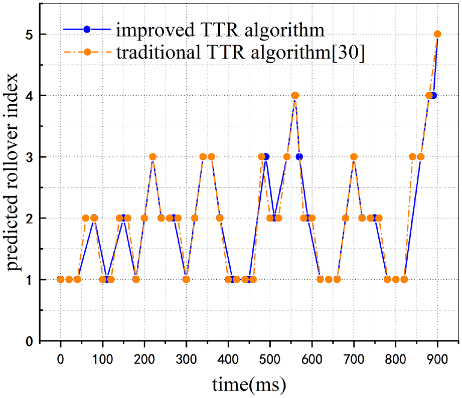
Results of one TTR prediction time.

It can be seen in Figure 8 that at the initial moment, the neural network predicts a rollover indicator of 1. For the improved TTR algorithm the next prediction is made at an interval of 40 ms, which meets the algorithm requirements, and the next prediction is made at an interval of 30 ms when the predicted indicator is 2, and so on for the later results. For the traditional TTR algorithm, no matter what the value of the predicted rollover indicator is, a fixed interval of 20 ms is taken for the next detection. It is not difficult to find that the traditional TTR method samples more points in this result because it takes a fixed step, especially when the value of the sidestep indicator is small, which is where the improved TTR algorithm has the advantage that using a variable step can reduce the number of samples and improve efficiency at low risk. In addition, it can be seen that although the number of samples is less than the traditional TTR method, the improved TTR algorithm is also able to grasp the trend and effectively detect the turning points at which the rollover indicator rises and falls. When it reaches 900 ms, the vertical coordinate is 5, which means that at this time the neural network predicts the rollover indicator to be 5. When the rollover condition is reached, both algorithms stop and the output TTR time is 900 ms.

To investigate the efficiency of the machine learning method, we recorded the time used for each step of the cycle during the training of the neural network, as shown in Figure 8. The computing platform we used is NVIDIA 1650ti GPU computing. The hyperparameters of the neural network we recorded for the training process are set as follows: $epochs = 250$ , $lr = 0.009$ , $batch size = 25$ .

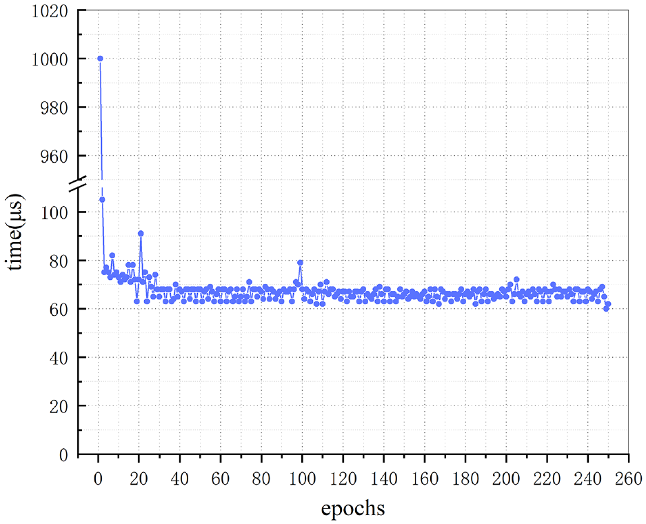
From Figure 9, it is easy to see that at the beginning of the training, the first two cycles consume relatively long time, 1 ms and 105 $μ s$ , respectively, after which most of the time used in the cycles is between 60 and 80. Compared with the traditional method of relying on the sensor test results to calculate the car rollover time, it is obvious that the method of using machine learning algorithms with the powerful arithmetic power of high-performance computers is more efficient and can reduce unnecessary time costs.

Figure 9.

Neural network training time.

Conclusions

For the rollover prevention of the new energy vehicle, the improved TTR with the neural network has been proposed by this paper. The parameters affecting rollover have been given through theoretical analysis. Combining the parameters of the new energy vehicle, multiple influencing factors have been given, and variable step size has been used. Finally, the influence of multiple hyperparameters for the multilayer neural network on the results has been analyzed, and the following conclusions can be obtained.

For the relationship between different hidden layers of the neural network and the prediction accuracy, the hidden layers have been considered as three layers.

For the effects of different number of cycles on the prediction accuracy, the neural network can obtain better accuracy under the conditions of and the number of cycles of training of the neural network also basically reaches the threshold, and the prediction accuracy finally tends to a stable value.

For the effects of different learning rates on the prediction accuracy, the accuracy is low at the beginning of the training cycle, and it needs nearly 160 cycles to reach stability, which indicates that the premise that can meet the requirements is basically the minimum value of the learning rate.

The batch size selected in the cyclic process at this time is larger, which will not only increase the calculation time, but also not get the expected accuracy rate, instead of gaining more than losing. Additionally, compared with the traditional method of relying on the sensor test results to calculate the car rollover time, the results shown that the method of using machine learning algorithms with the powerful arithmetic power with high-performance computers is more efficient, and can reduce the time costs.

Footnotes

Declaration of conflicting interests

The author(s) declared no potential conflicts of interest with respect to the research, authorship, and/or publication of this article.

Funding

The author(s) disclosed receipt of the following financial support for the research, authorship, and/or publication of this article: This work is supported by the Natural Science Foundation of Hunan Province (2021JJ30083) and State Key Laboratory of Advanced Design Manufacturing for Vehicle Body (71865009).

ORCID iD

Hong-Liang Dai

References

Bei

. Research method of vehicle rollover mechanism under critical instability condition. Adv Mech Eng 2019; 11(1): 1–11.

National Highway Traffic Safety Administration. 2015 motor vehicle crashes: overview. Traffic Safety Facts Res 2016; 2016: 1–9.

Lee

Yakub

Kasahara

, et al. Rollover prevention with predictive control of differential braking and rear wheel steering. In: 2013 6th IEEE conference on robotics, automation and mechatronics (RAM), Manila, Philippines, 12–15 November 2013, pp.144–149. New York, NY: IEEE.

Ervin

. Cooperative agreement to foster the deployment of a heavy vehicle intelligent dynamic stability enhancement system. 1998.

Chen

Peng

. Differential-braking-based rollover prevention for sport utility vehicles with human-in-the-loop evaluations. Veh Syst Dyn 2001; 36(4–5): 359–389.

Chen

. Warning and control for vehicle rollover prevention. Ann Arbor, MI: University of Michigan, 2001.

Zong

Miao

Zhang

, et al. Research on rollover warning algorithm of heavy commercial vehicle based on prediction model. In: 2010 IEEE international conference on computer, mechatronics, control and electronic engineering, Changchun, China, 24–26 August 2010, vol. 4, pp.432–435. New York, NY: IEEE.

Zhou

Zhu

, et al. Study on busses rollover warning based on roll angle threshold. In: 2010 2nd international conference on industrial and information systems, Dalian, China, 10–11 July 2010, vol. 1, pp.219–222. New York, NY: IEEE.

Rajamani

Piyabongkarn

Tsourapas

, et al. Real-time estimation of roll angle and CG height for active rollover prevention applications. In: 2009 American control conference, St. Louis, MO, USA, 10–12 June 2009, pp.433–438. New York, NY: IEEE.

10.

Zong

, et al. Anti-rollover control algorithm for heavy semi-trailer based on LQG. In: 2010 IEEE international conference on information and automation, Harbin, China, 20–23 June 2010, pp.1593–1596. New York, NY: IEEE.

11.

Zhao

Yang

, et al. A design method of EV charging security early warning model. In: 2017 36th Chinese control conference (CCC), Dalian, China, 26–28 July 2017, pp. 26–30. New York, NY: IEEE.

12.

Yang

. 3D convolutional neural networks for human action recognition. IEEE Trans Pattern Anal Mach Intell 2013; 35(1): 221–231.

13.

Zeng

Xie

Chen

, et al. Adaptive population extremal optimization-based PID neural network for multivariable nonlinear control systems. Swarm Evol Comput 2019; 44: 320–334.

14.

Chen

Zeng

, et al. A two-layer nonlinear combination method for short-term wind speed prediction based on ELM, ENN and LSTM. IEEE Internet Things J 2019; 6: 6997–7010.

15.

Chen

Buehler

. De novo composite design based on machine learning algorithm. Extreme Mech Lett 2018; 18: 19–28.

16.

Zhang

Liu

, et al. Battery fault diagnosis for electric vehicles based on voltage abnormality by combining the long short-term memory neural network and the equivalent circuit model. IEEE Trans Power Electron 2021; 36(2): 1303–1315.

17.

Abueidda

Almasri

Ammourah

, et al. Prediction and optimization of mechanical properties of composites using convolutional neural networks. Compos Struct 2019; 227: 111264.

18.

Belge

Altan

Hacıoğlu

. Metaheuristic optimization-based path planning and tracking of Quadcopter for payload hold-release mission. Electronics 2022; 11: 1208.

19.

Altan

Aslan

Hacıoglu

. Real-time control based on NARX neural network of hexarotor UAV with load transporting system for path tracking. In: 2018 6th international conference on control engineering & information technology (CEIT), Istanbul, Turkey, 25–27 October 2018, pp. 435–441. New York, NY: IEEE.

20.

Yang

Yabansu

Al-Bahrani

, et al. Deep learning approaches for mining structure-property linkages in high contrast composites from simulation datasets. Comput Mater Sci 2018; 151: 278–287.

21.

Rao

Liu

. Three-dimensional convolutional neural network (3D-CNN) for heterogeneous material homogenization. Comput Mater Sci 2020; 184: 109850.

22.

Chen

. Effect of constituent materials on composite performance: exploring design strategies via machine learning. Adv Theory Simul 2019; 2(6): 1900056.

23.

Chen

Peng

. Rollover warning for articulated heavy vehicles based on a time-to-rollover metric. J Dyn Syst Meas Control 2005; 127(3): 406–414.

24.

Treetipsounthorn

Phanomchoeng

. Real-time rollover warning in tripped and un-tripped rollovers with a neural network. In: 2018 IEEE 4th international conference on control science and systems engineering (ICCSSE), Wuhan, China, 21–23 August 2018, pp. 95-100. New York, NY: IEEE.

25.

Dong

Jiang

Zhong

, et al. An improved rollover index based on BP neural network for hydropneumatic suspension vehicles. Math Probl Eng 2018; 2018: 1–15.

26.

Zhu

Piao

Zhao

, et al. Integrated chassis control for vehicle rollover prevention with neural network time-to-rollover warning metrics. Adv Mech Eng 2016; 8(2): 1–13.

27.

Zhu

Yin

, et al. Research on a novel vehicle rollover risk warning algorithm based on support vector machine model. IEEE Access 2020; 8: 108324–108334.

28.

Chen

Zhao

Kong

, et al. Research on battery box lightweight based on material replacement. In: 5th international conference on mechatronics, materials, chemistry and computer engineering (ICMMCCE), Chongqing, China, 24-25 July 2017, pp.346–358. Atlantis Press. doi:10.2991/icmmcce-17.2017.72.

29.

Zhao

Guo

Zhu

, et al. Rollover warning for light vehicles based on NN-TTR algorithm. J Jilin Univ (Eng Technol Ed) 2012; 42(5): 1083–1088.

30.

Zhu

Zong

, et al. Rollover warning system of heavy duty vehicle based on improved TTR algorithm. J Mech Eng 2011; 47(10): 88–94.

31.

Chen

Liu

Wang

, et al. A rollover warning algorithm for improving steering wheel angle TTR and dynamic mass centroid height. Mech Sci Technol Aerospace Eng 2018; 37(4): 623–628.

Warning model of new energy vehicle under improving time-to-rollover with neural network

Abstract

Keywords

Introduction

Establishment of model and character recognition

Three-degree-of-freedom car model

Selection of rollover warning index

Improved TTR method

Numerical examples and discussion

Effect of the number of hidden layers on prediction accuracy

Effect of number of epochs on prediction accuracy

Impact of learning rate on prediction accuracy

Effect of different batch sizes on prediction accuracy

Analysis and validation

Conclusions

Footnotes

Declaration of conflicting interests

Funding

ORCID iD

References