
Abstract
This study proposes an integrated docking approach for autonomous underwater vehicle (AUV), which directly generate control force and torque from visual guidance features to drive precise AUV docking. Accurate docking control has been constructed as nonlinear offset-free model predictive control (OFNMPC) problem to effectively deal with external disturbances, model mismatch, and various other constraints. For the problem of state and disturbance estimation required by OFNMPC, observers have been presented based on the extended Kalman filter (EKF) and moving horizon estimation (MHE). A visual observation model is proposed so that the observer can directly use visual measurements. OFNMPC was integrated with EKF and MHE, and the proposed OFNMPC-EKF and OFNMPC-MHE docking approaches were applied to an actual AUV model. The simulation results show that the proposed approaches could drive the AUV to complete accurate docking along a reasonable trajectory based on visual measurements. The navigation, guidance, and control functions of docking were effectively integrated. It was observed that in the presence of external disturbances and measurement noise, OFNMPC-EKF has better robustness.
Keywords
Introduction
The transition of an autonomous underwater vehicle (AUV) from a state of free travel to being physically connected to another station or platform is called docking. 1 AUV can dock to underwater station, such as standalone docking station (DS) carrying large capacity energy or underwater network node, to get energy supplement. This enables the AUV to reside and operate underwater for long durations. In addition, automatic recovery can be realized based on docking technology, and an AUV can become an automatic tool for larger surfaces or underwater vehicles. Owing to the significance of docking technology in the expansion of AUV applications, it has become a research hotspot in the field of AUV technology since the 1990s.
The fundamental elements of AUV docking are guidance, navigation and control components. 2 The navigation integrates sensor information to estimate the state required for docking guidance and control, such as, the position, attitude and velocity of the AUV relative to the DS. A large number of filtering algorithms are used for AUV integrated navigation, such as, the extended Kalman filter (EKF),3,4 unscented Kalman filter (UKF), 5 particle filter (PF), 6 Sum of Gaussian (SoG) filter, 7 and fuzzy Q-learning. 8 Navigation sensors typically include Doppler velocity logs (DVL), inertial navigation systems (INS), and pressure sensors. The position of an AUV relative to the DS is typically obtained using acoustic equipment or vision methods.3,9–13 The vision-based approach extracts guidance features from underwater images, based on which, the position and attitude of an AUV are estimated. The update rate and accuracy of visual positioning are higher and it is typically used in the terminal stage of docking.
According to the navigation information, an AUV uses a certain strategy to guide and control itself into the DS. In general, the guidance law generates the motion target or feasible docking trajectory of the AUV, and the controller executes the command or tracks the trajectory to drive the AUV to the DS. Typical guidance laws include, pure pursuit, 14 line-of-sight (LOS), 15 and optimal control. 16 Some studies have considered the effects of ocean currents.17,18 The methods of docking trajectory planning include inverse dynamics in the virtual domain (IDVD), 19 geometric analysis, 20 and curve fitting. 21 Docking control methods include a variety of improved PID controls,17,22,23 sliding mode control, 24 backstepping control, 20 adaptive robust control law, 25 model-free robust control, 26 and neural network adaptive controller. 27
However, only a few studies have focused on a unified docking approach. This makes the systematic design and integral optimization of AUV docking difficult. Model predictive control (MPC) is an architecture that integrates guidance and control. The predicted state and input trajectory are generated by solving the optimization problem and the first item of the input trajectory is applied to the controlled plant.28,29 By constructing a constraint optimization problem, MPC can deal well with various constraints, such as, actuator ability, position and field of view (FOV) limits of the AUV in the docking process. 30 There have been some studies on the application of MPC to AUV docking.31–33 However, the AUV has strong coupling, high nonlinearity, and parameter uncertainty; therefore, it is difficult to obtain an accurate prediction model. 34 To solve the problems of model mismatch and external disturbance, nonlinear offset-free model predictive control (OFNMPC) has been proposed.35–39 OFNMPC uses an observer to estimate the state and disturbance. According to the disturbance estimation and reference, an equilibrium problem is constructed, which is added to the optimization problem to realize zero-offset control. OFNMPC has been applied to the docking of AUV in two previous studies.40,41Both the studies assume that the navigation system can provide direct position and attitude measurements. Intuitively, the observer function of OFNMPC can be extended such that it can directly use visual measurements to estimate the state and disturbance of the docking process. A method for camera pose estimation based on the EKF has been proposed 42 ; however, it does not include the dynamics model and cannot be used to estimate the disturbance. Compared with the EKF, the moving horizon estimation (MHE) can directly use an exact nonlinear model,43,44 and can be considered to realize the required observer.
Motivated by the aforementioned overviews, the aim of this study is to propose an integrated approach to AUV docking based on OFNMPC. The navigation, guidance, and control modules of docking were integrated into the framework, as shown in Figure 1. In the presence of measurement noise, external disturbances and model mismatch, the proposed approach should drive the AUV to achieve accurate docking and various constraints in the docking process can be met simultaneously. The approach is planned to be applied to an AUV driven by multiple propellers, which was developed for the scientific investigation of ocean trenches.
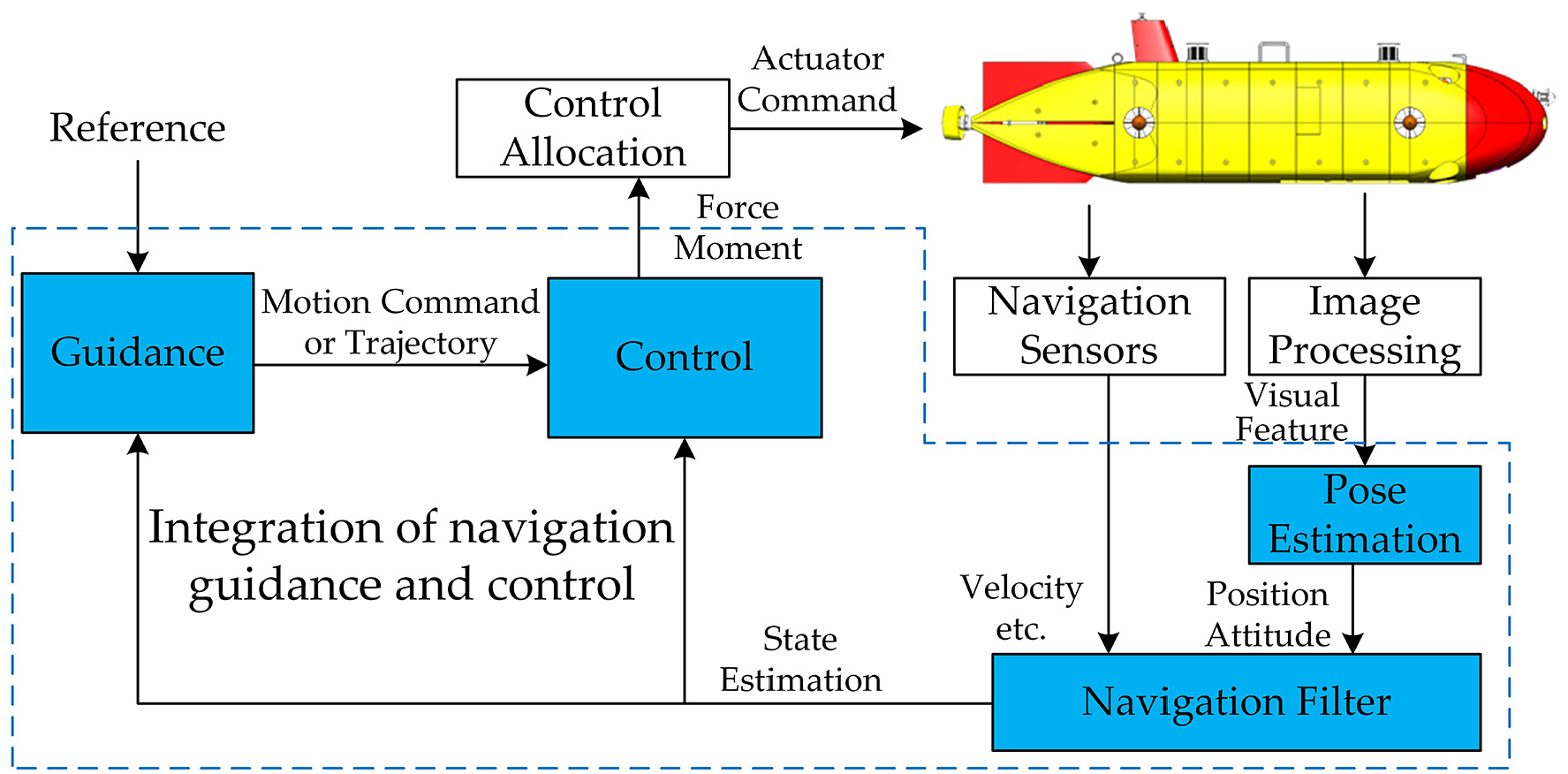
Typical AUV docking architecture (part enclosed in the blue dotted line was integrated using the proposed approach).
The main contributions of this study are summarized as follows: (1) A docking approach based on OFNMPC is proposed, which can effectively deal with external disturbances, model mismatch, and multiple constraints. (2) The OFNMPC observer was realized using EKF and MHE. The visual guidance features were fused directly by the observer to estimate the state and disturbance of the docking process. (3) A real multi-propellers AUV model was used as the controlled plant, and the effectiveness and robustness of the proposed approaches were verified through simulations in multiple scenarios. (4) The effects of docking in OFNMPC-EKF and OFNMPC-MHE were compared, and the results were analyzed.
The remainder of this paper is organized as follows: Section 2 introduces the AUV docking system and describes the problem of offset-free docking. Section 3 presents the design methods of OFNMPC-EKF and OFNMPC-MHE. The simulation results and analysis are presented in Section 4. Finally, the conclusions are presented in Section 5.
Problem statement
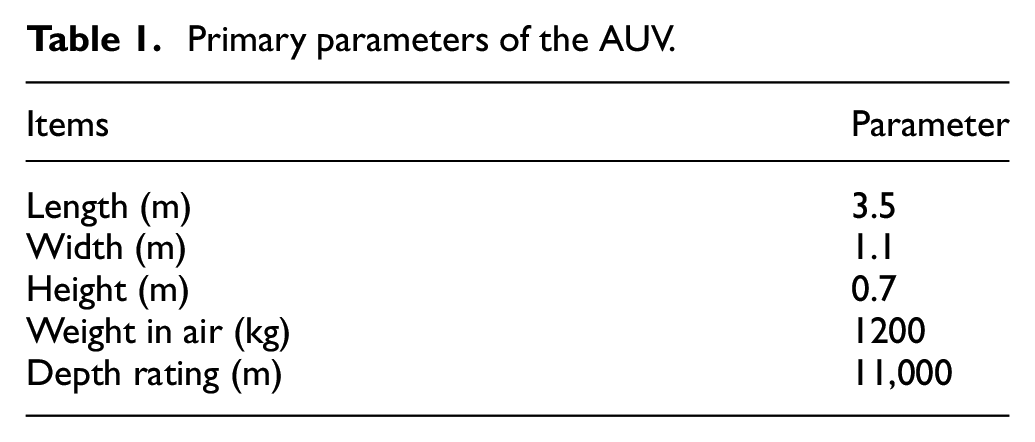
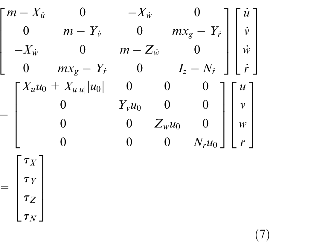
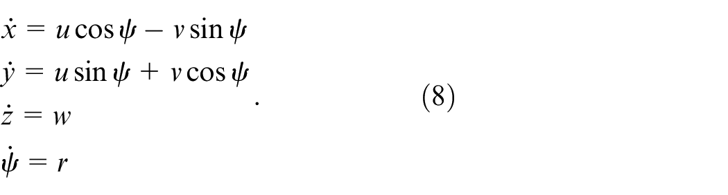
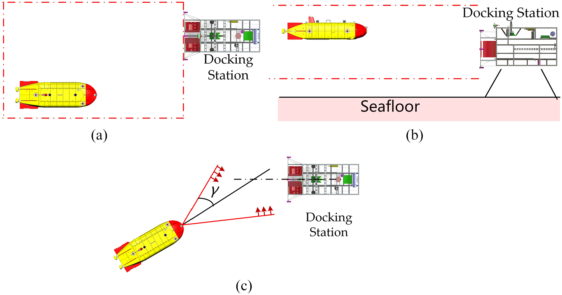
The docking system included a fully actuated AUV and DS placed on the seafloor. The AUV had a depth rating of 11,000 m and was developed for scientific investigation of ocean trenches and long-term residence. Seven thrusters were installed on the AUV, as shown in Figure 2. The AUV had six degrees-of-freedom of motion. The main parameters of the AUV are listed in Table 1. Six underwater lights were symmetrically installed around the entrance of the DS to obtain significant visual guidance features. A camera was installed on the AUV to capture underwater images. A special visual processing module was used to extract the point features from underwater images. In addition, the AUV was equipped with INS and DVL and the linear and angular velocities of the AUV could be measured.
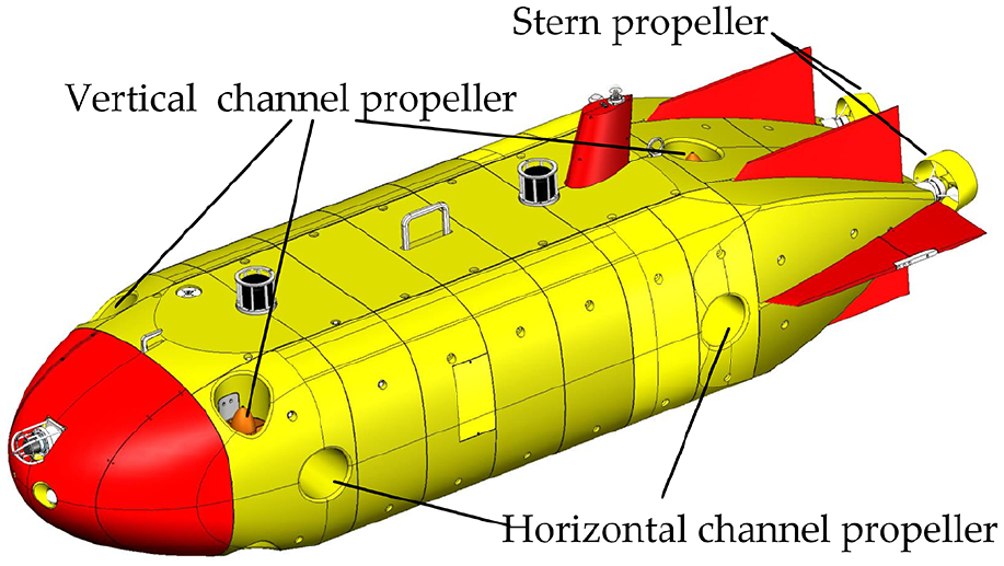
AUV propulsion configuration.
Primary parameters of the AUV.
It is convenient to define the DS coordinate frame and body-fixed reference frame as indicated in Figure 3. In addition, a camera coordinate system is needed for the analysis of visual information. The DS coordinate system
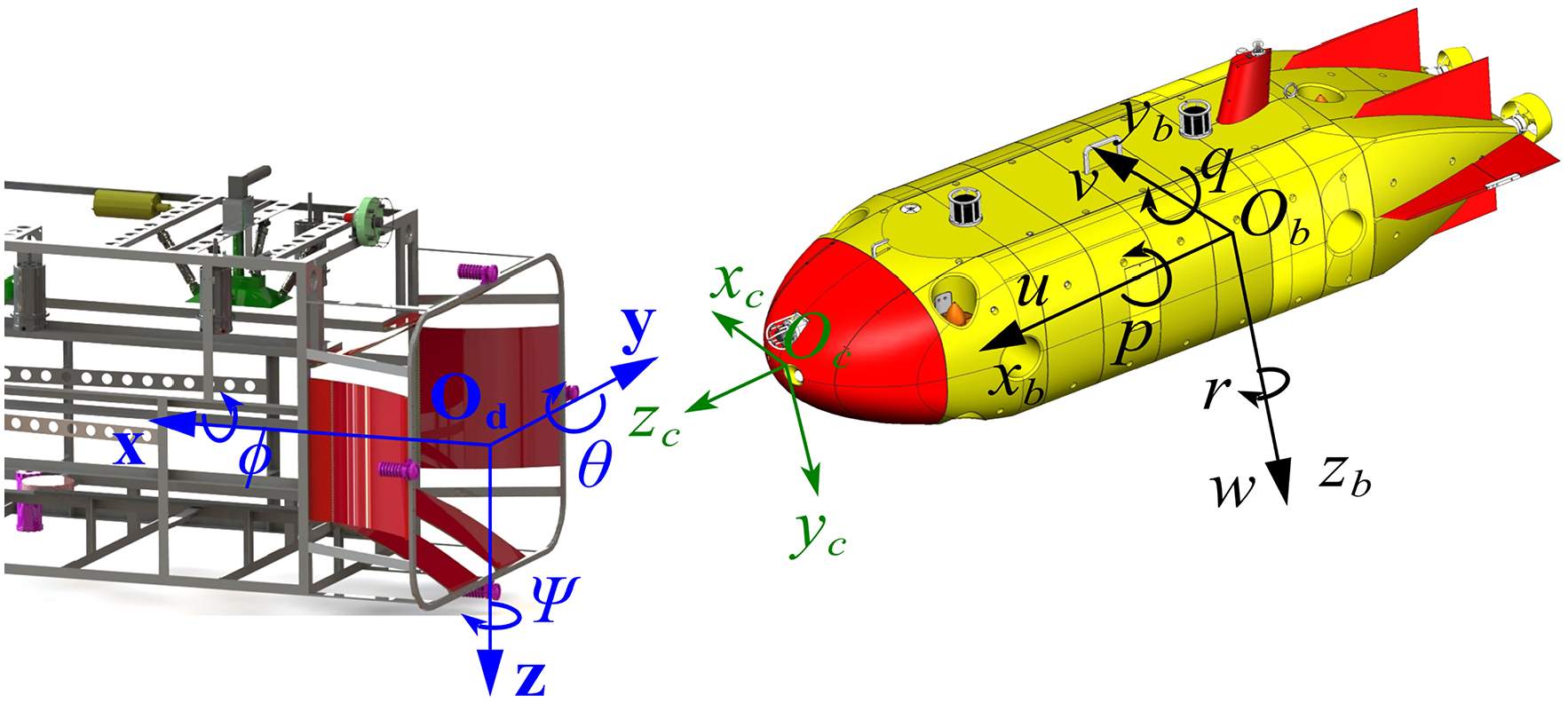
Coordinate system for AUV docking.
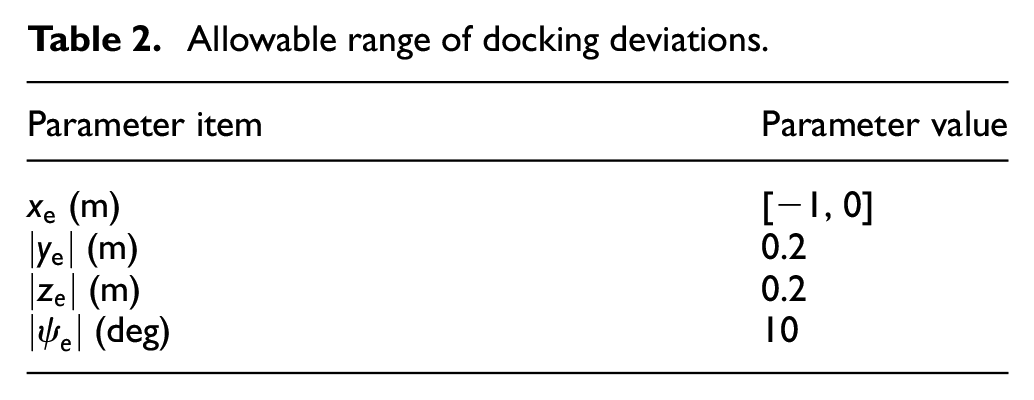
A The AUV approaches the DS from a distance and docks after recognizing the underwater light. This study focuses on the docking stage. In the case of docking to a static DS, the goal is that the AUV reaches the entrance of the DS and its attitude is consistent with that of the DS. The guide cover at the entrance of the DS was designed to be funnel shaped to provide a fault-tolerant space to the AUV for docking. If the arrival deviation of the AUV is within the allowable range, it can be regarded as a successful docking. The allowable deviations in the
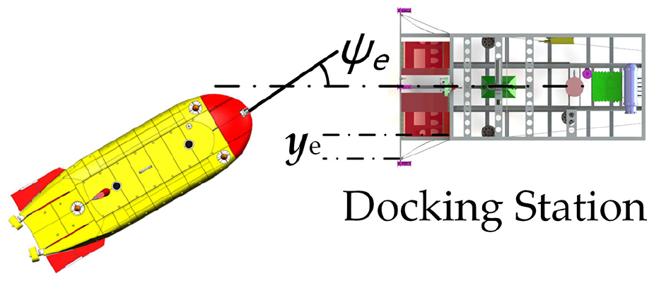
Schematic of docking allowable deviations in the horizontal plane.
Allowable range of docking deviations.
The docking process is affected by the external disturbances and measurement noise. The dynamic model of the AUV used for the design is inaccurate; therefore, the AUV docking task includes the following three aspects.
The state and disturbance of the docking process can be effectively estimated based on the measurements with noise.
Steering the AUV to the DS accurately to meet the allowable deviation requirements, even if there are external disturbances and model mismatch.
The trajectory of AUV reaching DS is reasonable and economical.
Docking approach design
In this section, the proposed docking approach is introduced. First, the architecture of the docking scheme is described briefly. The designs of the OFNMPC and the two observers are explained. Finally, the method to integrate the OFNMPC and observer is proposed.
Docking scheme considerations
Figure 5 shows the architecture of the docking approach, which is primarily composed of the OFNMPC and observer (portion in blue). The velocity measurements of the sensors and visual features extracted from the images are provided to the observer. Combined with the control input from the OFNMPC, the state and external disturbances of the system are estimated by the observer. The OFNMPC outputs the force and torque commands to complete the closed-loop control. Our study does not include control allocation; however, some methods can be applied. 45
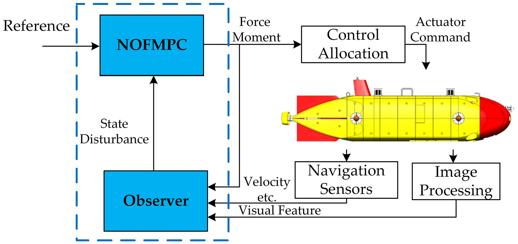
Architecture of the docking approach.
Nonlinear offset-free model predictive control
Prediction model
The dynamics of an AUV are highly nonlinear and coupled and its vector representation of the nonlinear equations of motion can be described as:

where
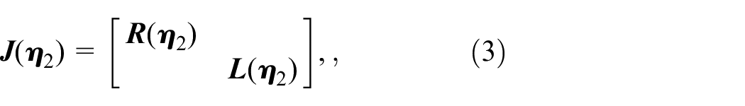
The kinematic model of an AUV can be written in concise matrix form as

The expressions for
where

and
Simplifying the dynamics model in equation (1), ignoring

The surge, sway, heave, and yaw, to be controlled by the OFNMPC are selected. The roll and pitch are controlled near zero using conventional controllers, which is reasonable if the DS is properly arranged on the seabed. The status
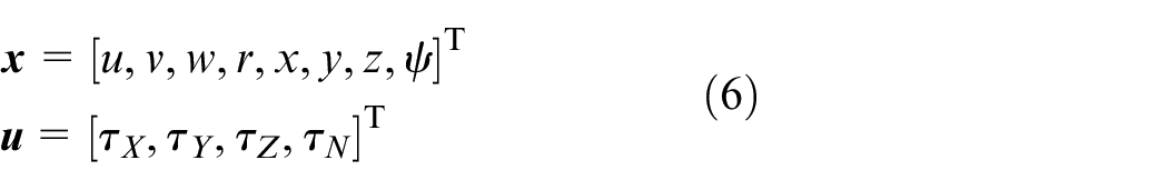
The nominal velocity vector
where m is the mass of the AUV and
The kinematic part of the prediction model is:
Constraints during docking
AUV actuators, such as, propellers and rudders, have ability limits, which can be described using input constraints as:

During docking, it is undesirable for the AUV to deviate too far from the DS and it is not allowed to enter the area behind the DS entrance or too close to the seabed. To obtain visual guidance, the DS must always remain within the FOV of the AUV camera. These constraints are shown in Figure 6, and represented by the inequality described in equation (10), with controller state

Examples of constraints during docking: (a) horizontal position constraint, (b) vertical position constraint, and (c) FOV constraint.
OFNMPC design
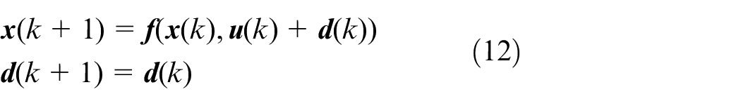
The prediction model composed of equations (7) and (8) is written in the function form after discretization as:

To address the problem of model mismatch and external disturbance, the disturbance variable
and the output model of the system is

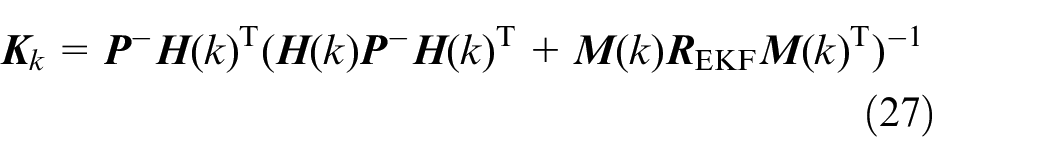
OFNMPC obtains the state estimation
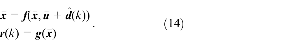
The target condition is integrated into the NMPC formulation as equality constraints, and there is no need to solve the analytical form of
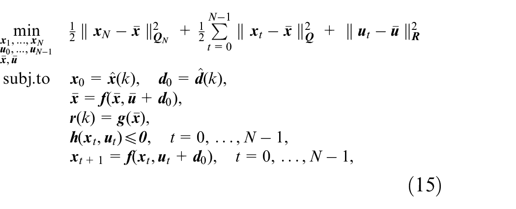
where

Here,
Disturbance and state observer
This section presents the design of the observers for OFNMPC, based on EKF and MHE. In addition, the visual observation model required by the observers is described.
Extended Kalman filter
The Kalman filter is an optimal estimator for cases, in which the process and measurement noise are zero-mean Gaussian. For the state estimation problem, if the motion model or sensor model is nonlinear, the EKF is widely used. A nonlinear model was approximated using its first-order Taylor expansion in the iterative process.
The augmented form of the model, as in equation (12), is used as the process model as:

where
The form of observation model is:

where
The EKF is initialized as:

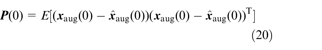
The estimation of the augmented state
The Jacobians
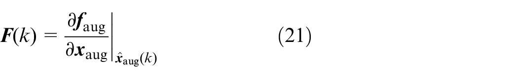
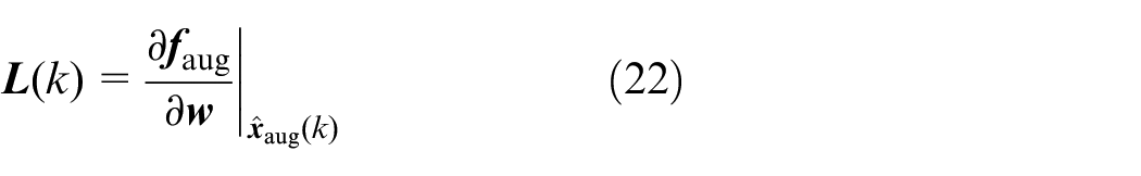
The prediction step can be written as:


The Jacobians
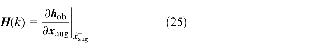
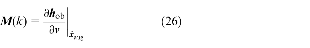
The updated steps of state estimation and the estimated error covariance are:


Moving horizon estimation
For an estimator under the framework of the Kalman filter, it is generally assumed that the system is Markov; that is, the current state contains the information of all the previous states. In contrast, the MHE transforms the state estimation problem into optimization problem constructed using window information and estimates the system state through nonlinear optimization. The MHE can directly use an exact nonlinear model, which is one of its advantages.
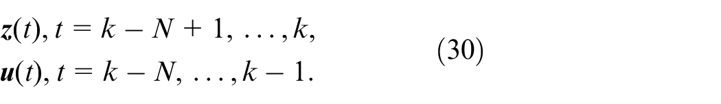
Considering the systems described in equation (11), at the current time k of the system, the input of the optimization problem includes N measurements and nominal control inputs closest to the current time as:
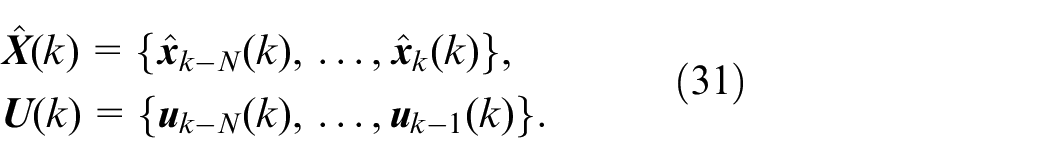
The system state and real input are used as optimization variables as:
A nonlinear optimization problem was constructed to estimate the state and input, where
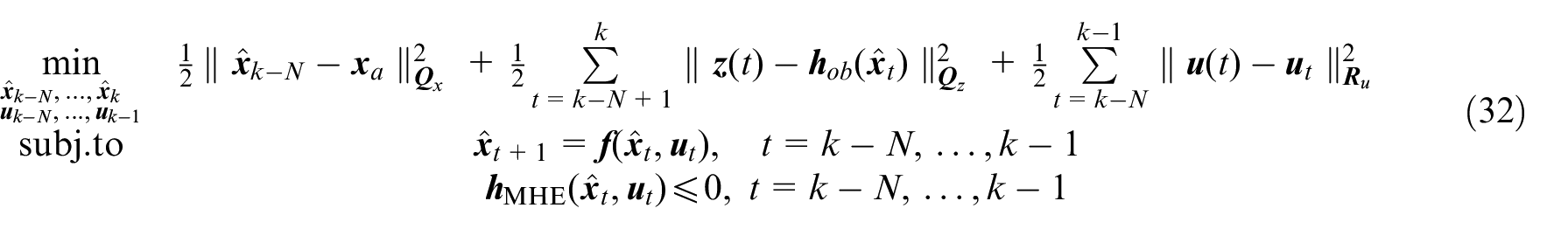
By solving the optimization problem, the state trajectory estimation
As only finite time domain data are used, the
Observation model
The visual observation model describes the relationship between the pixel coordinates of the visual features and the system state
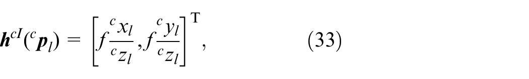
where f is the focal length of the camera.
The position of the AUV in

where

The transformation relationship in the visual observation model is illustrated in Figure 7.
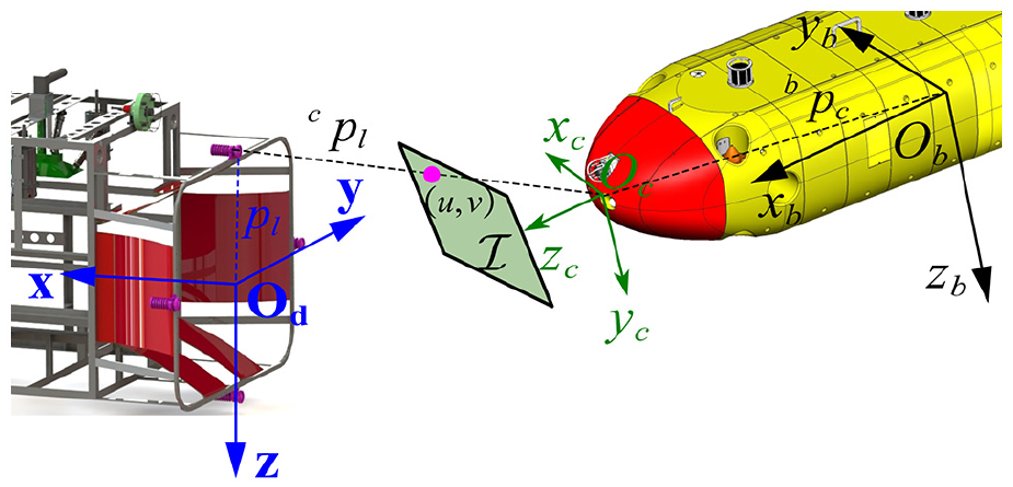
Schematic of the transformation relationship of the observation model.
The observation model can be used directly by MHE. The EKF requires the Jacobian of the observation model to estimate the Kalman gain and posteriori estimated error covariance. The EKF uses an augmented model, and the Jacobian is derived according to equations (35) and (25).
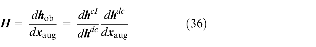
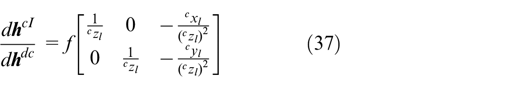
According to equation (33), we can obtain:
The augmented state consists of velocity, pose, and disturbance. Defining the pose of the AUV as
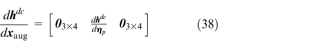
The form of
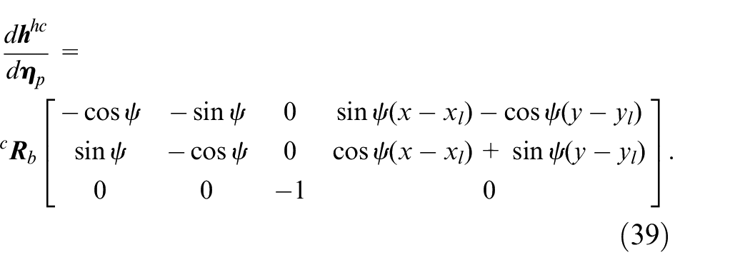
A visual observation model and its Jacobian have been presented. The observation model of velocity is linear and can be easily combined with equations (35) and (36) for the EKF and MHE.
Integrated OFNMPC and observer
The AUV is a continuous-time dynamic system that must be discretized. In this study, integration over one shooting interval was performed using the Runge-Kutta method, and a numerically approximate discrete system model was obtained. Several methods for model discretization are described in Gros et al. 46
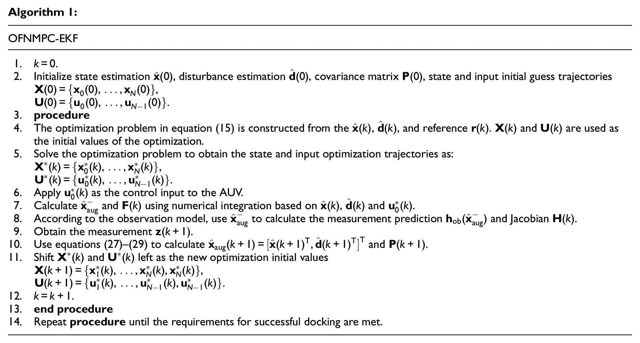
The OFNMPC-EKF is a natural method. The EKF is designed with an augmented model and provides state and disturbance estimations for the OFNMPC. The implementation of OFNMPC-EKF is described in Algorithm 1.
In MHE, we use the original prediction model instead of the augmented model. Algorithm 2 describes the implementation of the OFNMPC-MHE.
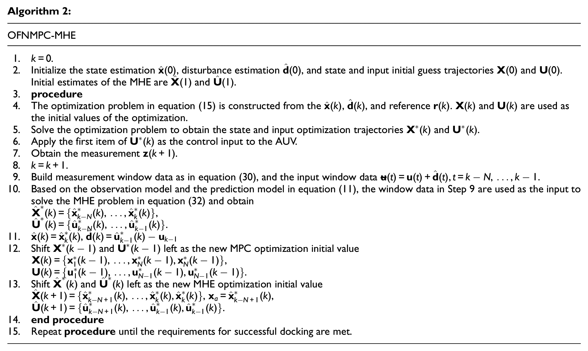
The input disturbance model used by OFNMPC is depicted in equation (12), and the use of Algorithm 2 does not affect the zero-offset control effect of the OFNMPC.
Simulation results and discussion
In this section, the proposed docking approaches, OFNMPC-EKF and OFNMPC-MHE, are applied to a fully actuated AUV, which was briefly introduced in Section 2. The model and parameter settings used in the simulation are explained, simulation results are presented and results are discussed.
Simulation model and parameter setting
A six degrees-of-freedom AUV motion model with full parameters was used as the controlled plant in the simulation. The disturbance of the ocean current was coupled in the model. The equations of motion, including ocean currents, are presented in (A6)–(A8) in Appendix A.
The dynamics part of the prediction model for docking control is shown in equation (7), and the specific form used for the simulation is as follows:
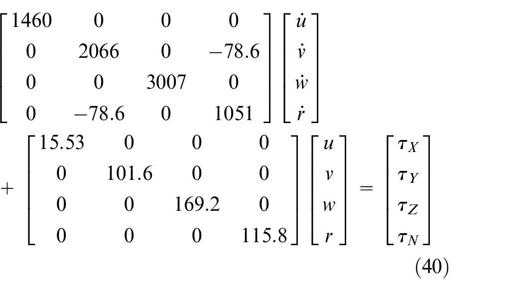
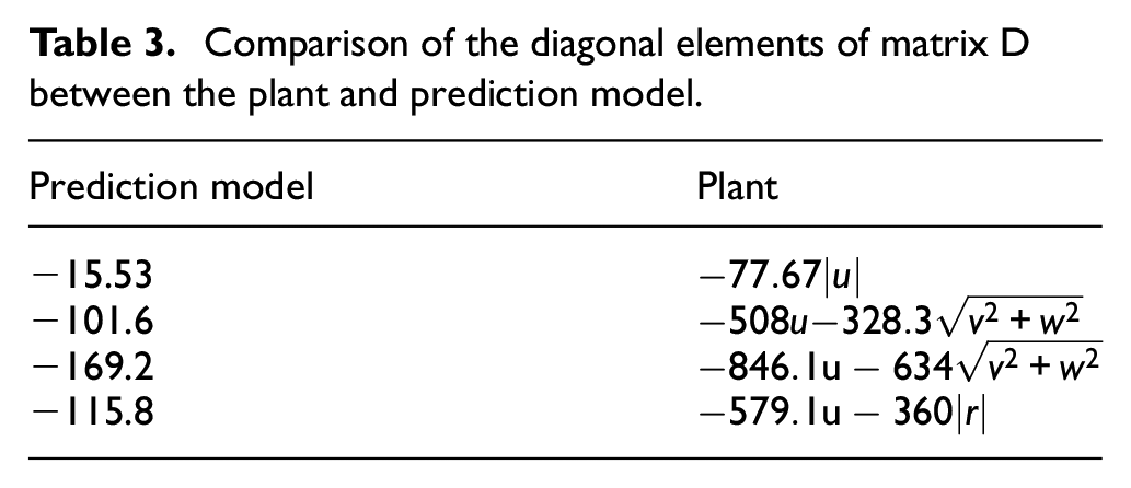
There was a distinct model mismatch between the prediction model and the controlled plant. This mismatch can be found by comparing the diagonal elements of matrix
Comparison of the diagonal elements of matrix D between the plant and prediction model.
The process models of EKF and MHE are the same as the prediction model of MPC, in which the EKF uses the augmented model. The observation models of EKF and MHE are introduced in Section 3.3.3.
In the simulation, the AUV started from the initial pose
In the simulation, six underwater lights were set as visual guidance. OFNMPC could obtain six pairs of pixel coordinates as the measurements. The resolution of the camera was
The prediction horizon of OFNMPC was
The process noise covariance matrix


The optimal horizon of MHE was
Both OFNMPC and MHE were constructed and solved using CasADi software framework. 47
Simulation results and analysis
Two simulation scenarios are designed to verify the effectiveness and robustness of the proposed method. In Scenario 1, the current disturbance and measurement noise were not added, and there was only a model mismatch to prove the feasibility of the proposed approach. In Scenario 2, the measurement noise and current disturbance were added to verify the robustness of the proposed approach. The effects of control of the OFNMPC-EKF and OFNMPC-MHE were compared and analyzed.
Scenario 1 with model mismatch
Figure 8 shows a comparison of the docking trajectories of OFNMPC-EKF and OFNMPC-MHE in Scenario 1. Both approaches drive the AUV to the set point. From the comparison of the output response of the three-dimensional position and heading shown in Figure 9, there is no distinct difference between the control effects of the two methods, except that the response of OFNMPC-MHE in the vertical direction is slightly slow. The estimation of the disturbance using the two methods is illustrated in Figure 10. Both methods obtained reasonable disturbance estimation results and accurately estimated the 10 N positive buoyancy in the steady state. It can be seen that OFNMPC realizes zero-offset docking control in the presence of a distinct model mismatch by estimating the disturbance.
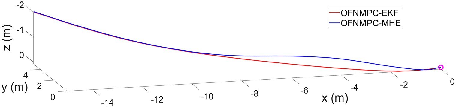
3D docking trajectory comparison in Scenario 1.
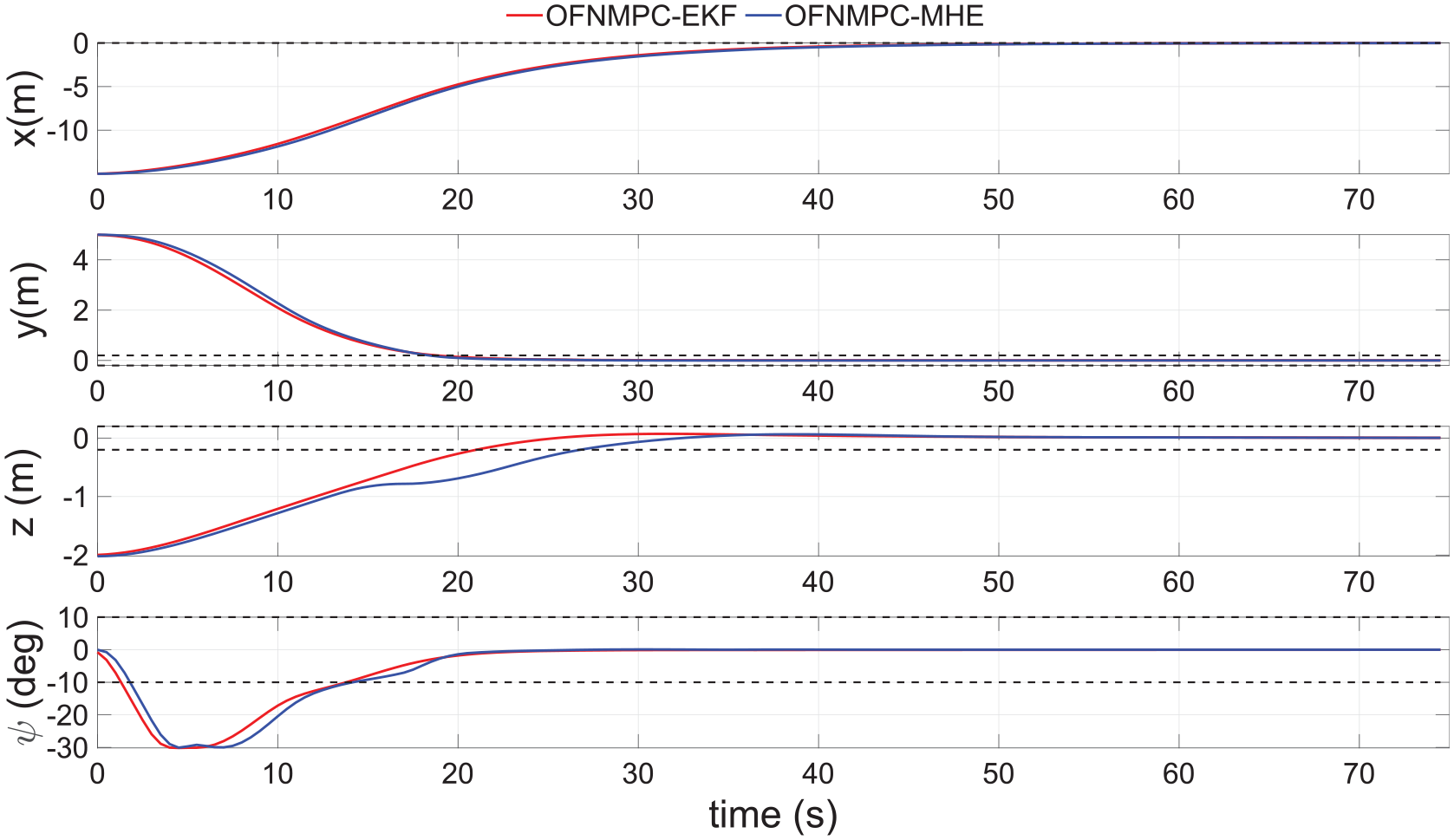
Output response comparison in Scenario 1 (dotted line indicates the allowable deviation).
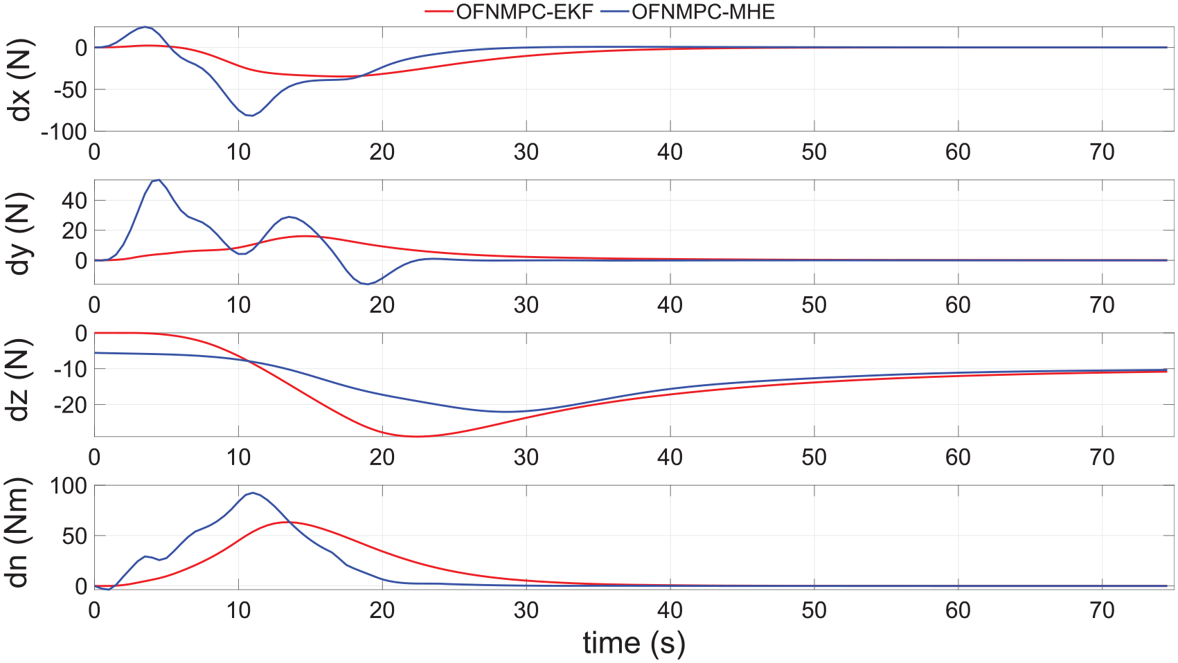
Disturbance estimation comparison in Scenario 1.
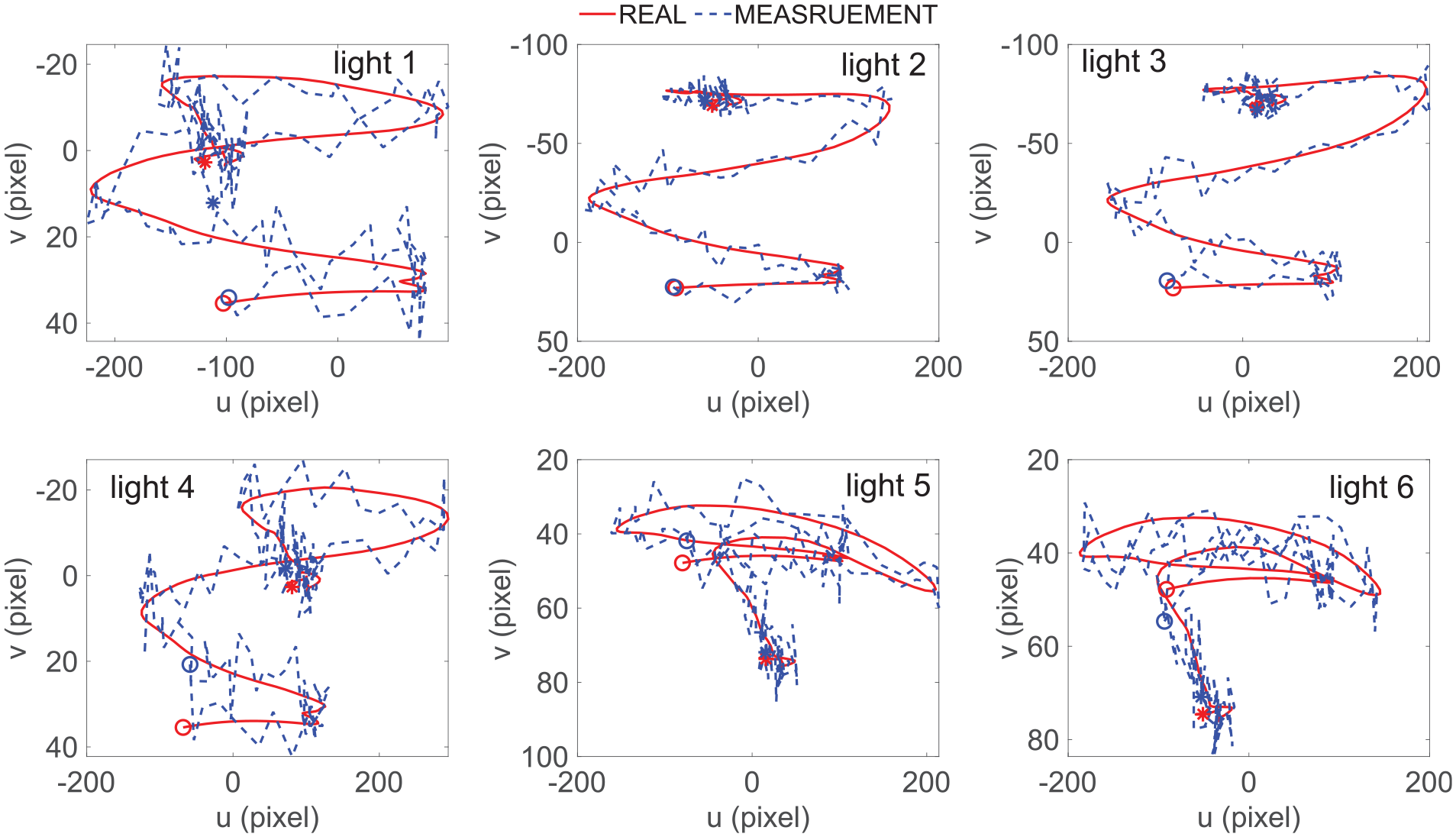
Figure 11 shows the trajectories of the visual features in the image plane, which were used as the measurements of the two approaches.
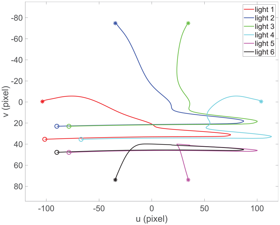
Trajectories of visual feature measurements on the image plane (O is the start point of the track, * is the end point of the track).
OFNMPC uses a fixed reference
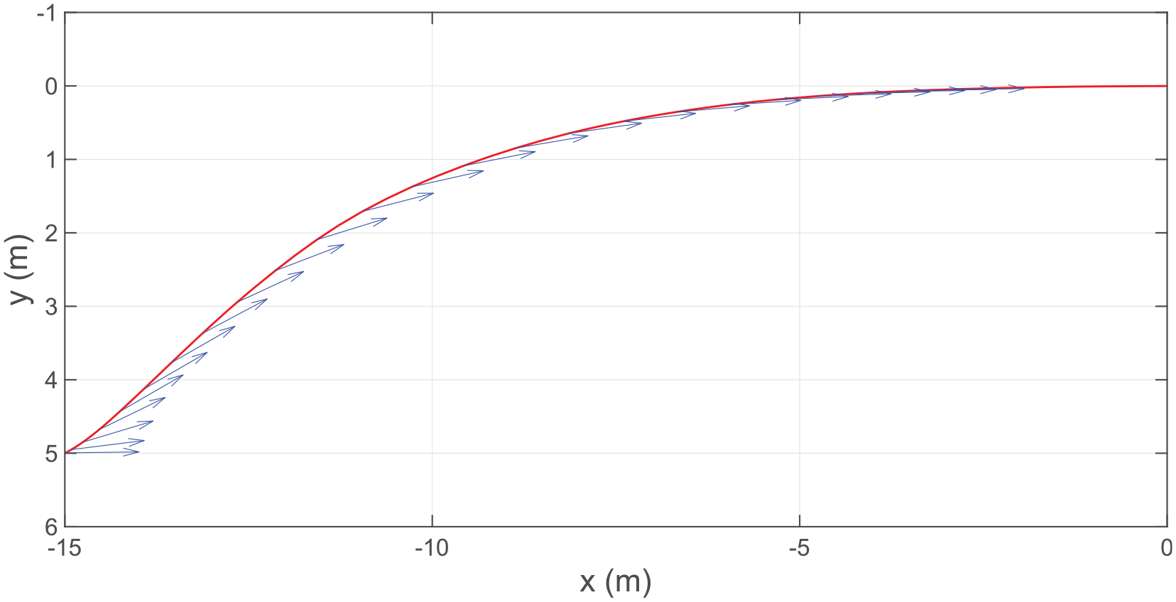
Horizontal docking path generated using OFNMPC-EKF (arrows indicate the heading of the AUV).
Scenario 2 with measurement noise and current disturbance
Current disturbance and measurement noise were added to the simulation. The maximum current was maintained at 0.3 m/s, and the angle of attack was
The random noise with standard deviation of 5 pixels was added to the visual feature measurements, and the random noise with standard deviation of 0.02 m/s was added to the horizontal velocity measurements. The measurements with noise are presented in Figures 13 and 14.
Vision measurements and their real trajectories (O is the start point of the trajectory, * is the end point of the trajectory).
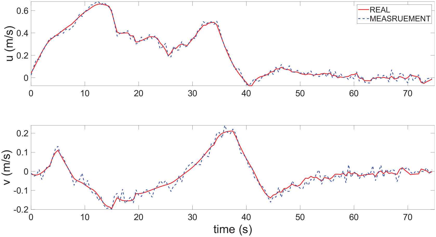
Velocity measurements and their real values.
Figures 15 and 16 show the 3D docking trajectories of OFNMPC-EKF and OFNMPC-MHE, respectively, under the interference of currents in five different directions. It can be observed that the OFNMPC-MHE has a large position deviation in two of the five simulations.
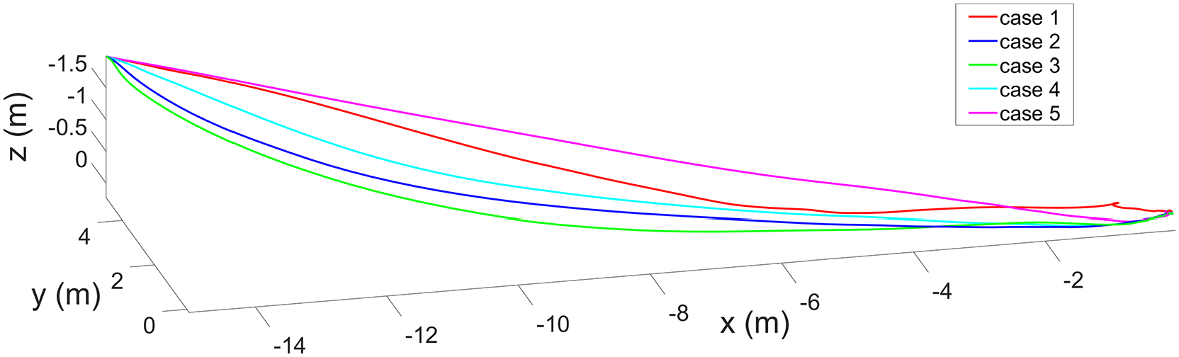
OFNMPC-EKF 3D docking trajectories in Scenario 2.
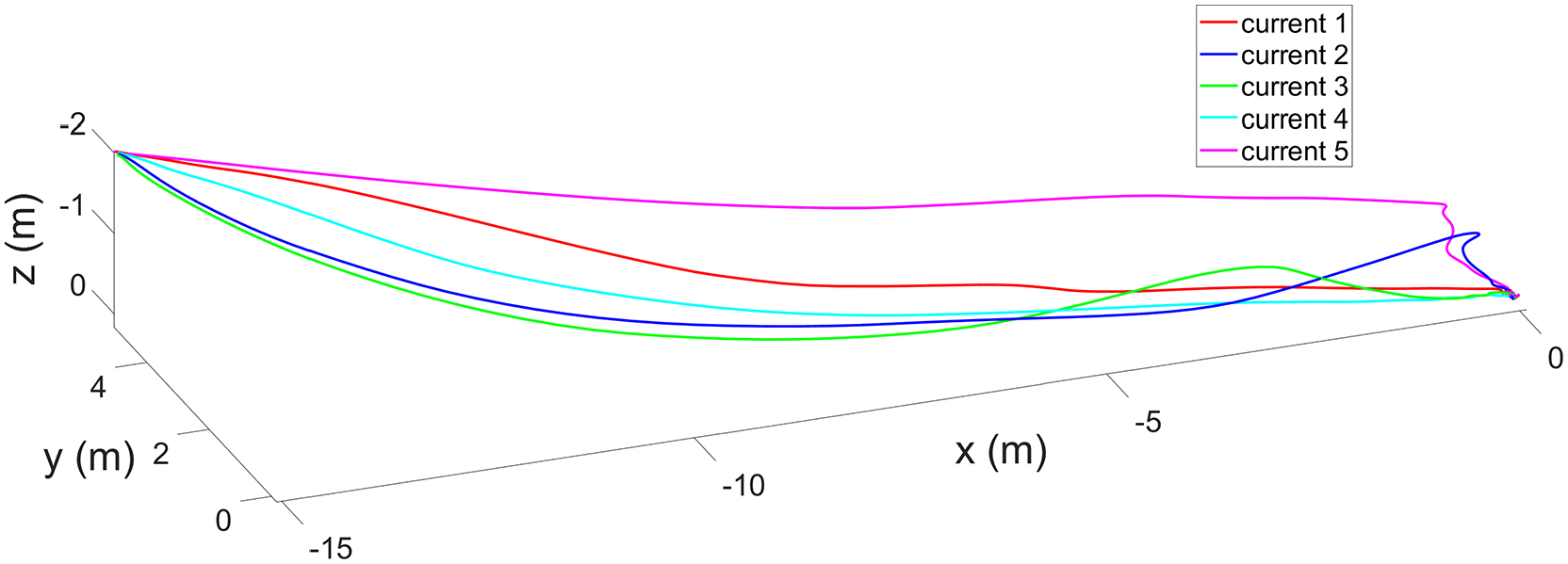
OFNMPC-MHE 3D docking trajectories in Scenario 2.
The time taken to drive the AUV from the initial position to the allowable deviation range is defined as the docking time. The docking times for the two approaches are compared in Table 4.
Comparison of docking time in Scenario 2.
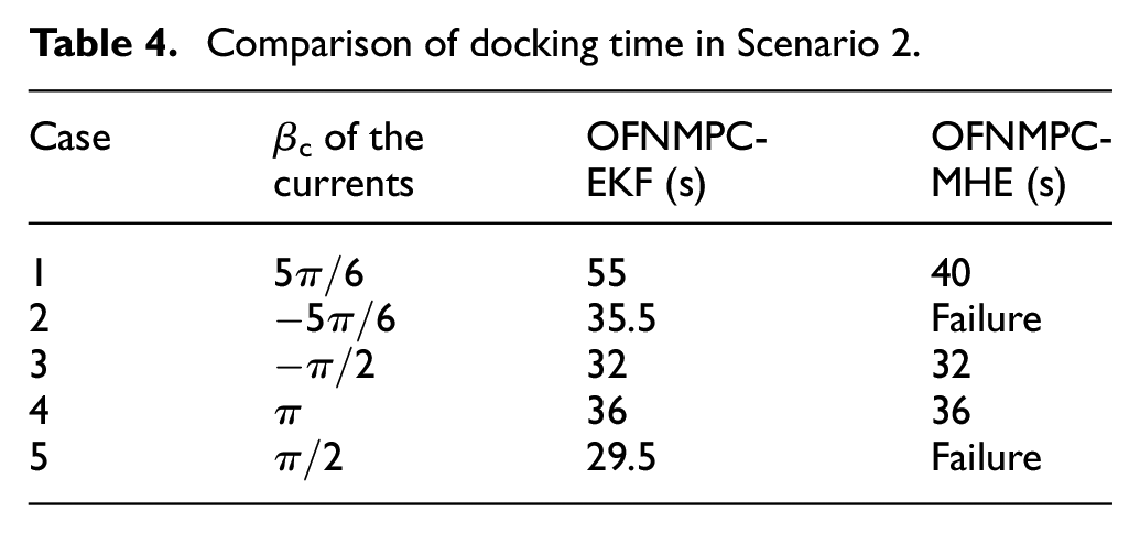
It can be observed that in the successful docking, the docking time of OFNMPC-MHE is slightly less than that of OFNMPC-EKF. For the case of failure, the simulation of case 2 was analyzed. The output response and disturbance estimation of the two approaches are shown in Figures 17 and 18, respectively. As shown in Figure 17, the disturbance estimation of the MHE to sway and yaw diverges over a period of time. The incorrect estimation of the external disturbance leads to a large amplitude swing in the bow direction of the AUV, which can be clearly seen in Figure 18. This causes the pilot light to move out of the camera FOV, resulting in a docking failure. Figure 19 shows a comparison of the control inputs. The input constraint was not broken. Similarly, an incorrect estimation of the MHE leads to the opposite control. Figure 20 shows a comparison of the pose estimation errors. Both EKF and MHE obtained accurate estimation results.
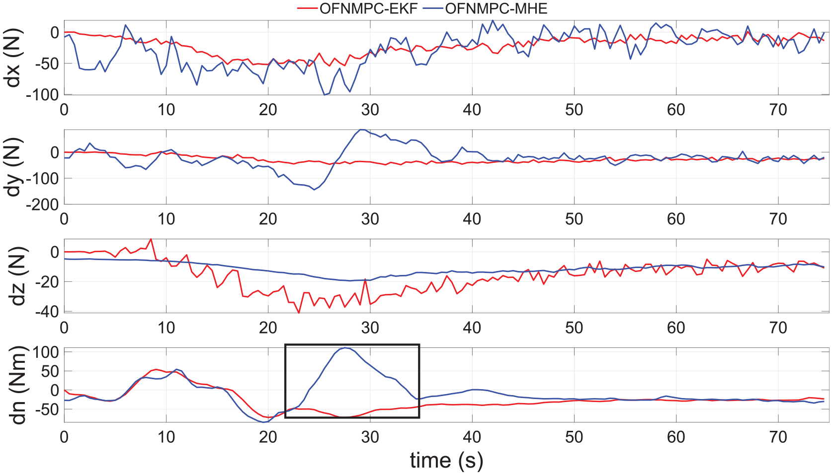
Disturbance estimation comparison in Scenario 2.
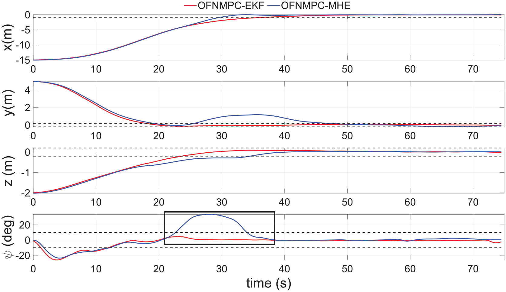
Output response comparison in Scenario 2 (dotted line indicates the allowable deviation).
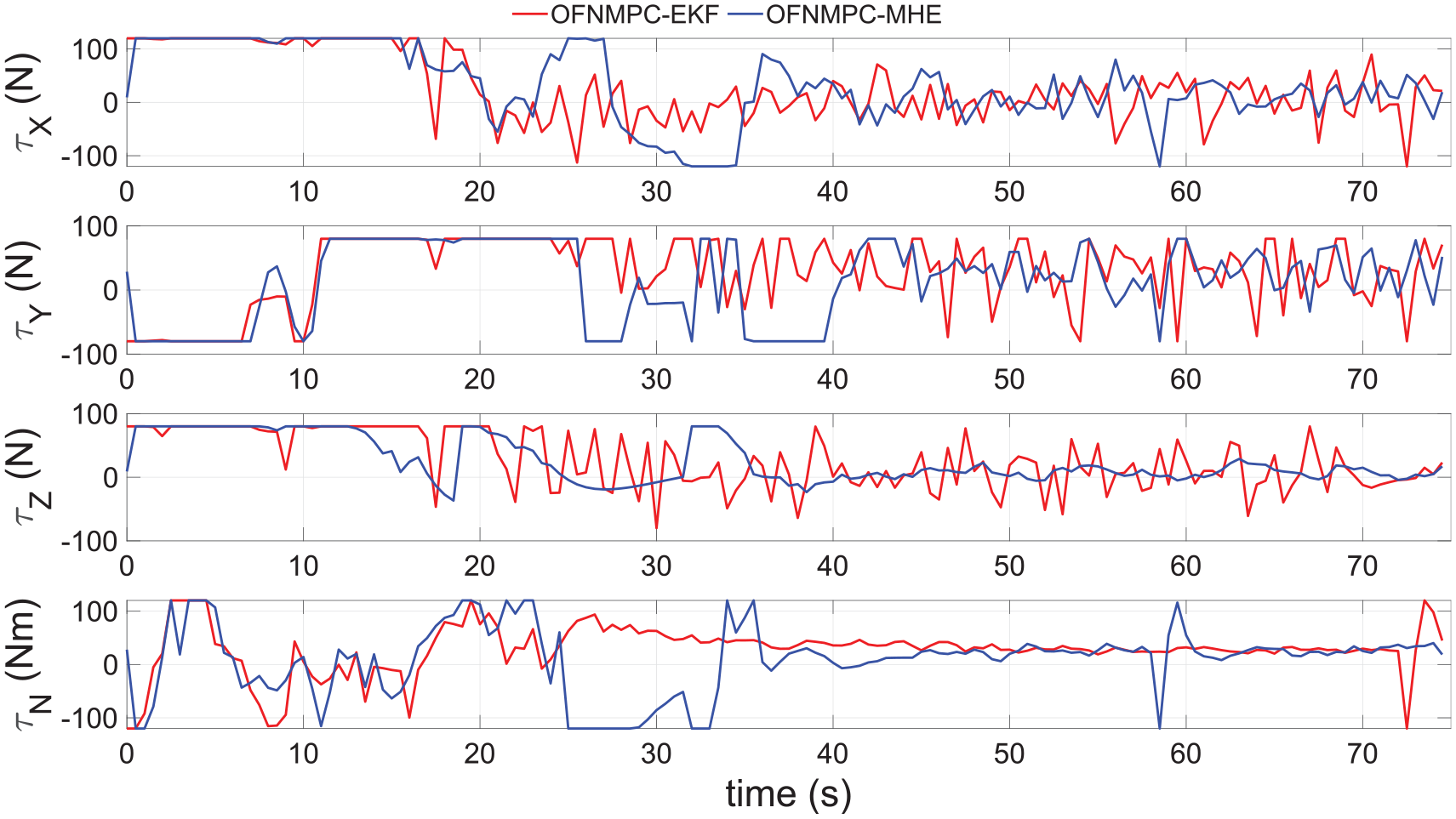
Control input comparison in Scenario 2.
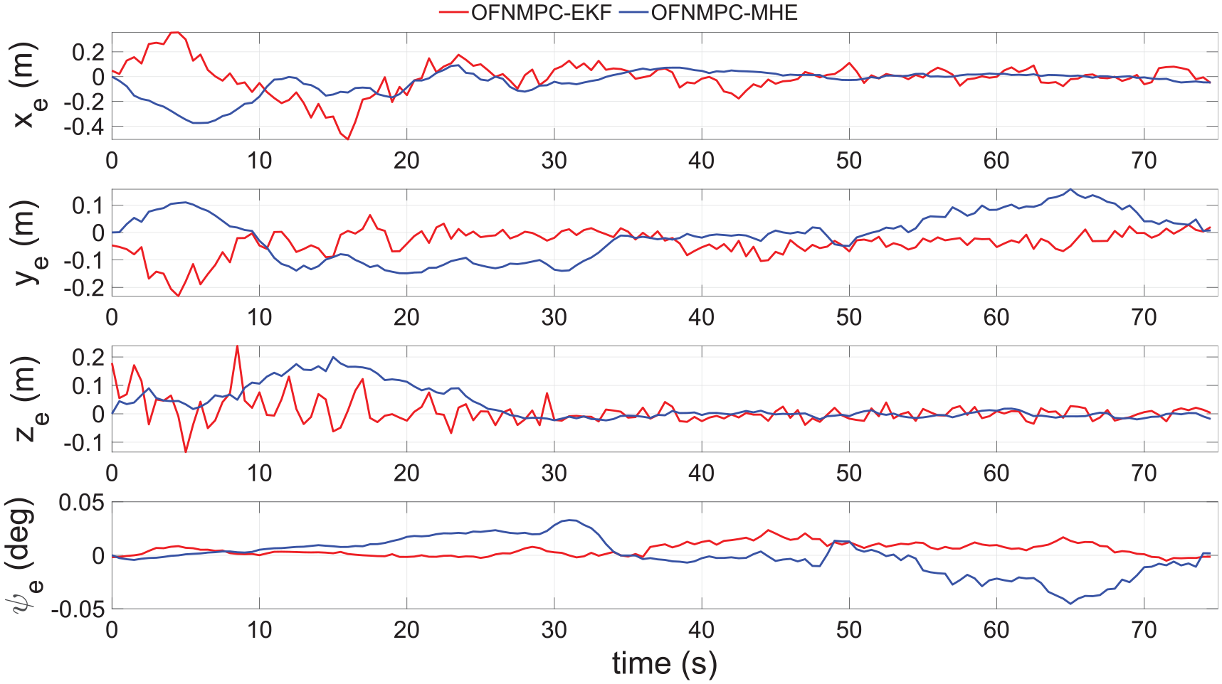
Pose estimation errors comparison in Scenario 2.
In this study, a simplified AUV dynamics model is used, which makes the MHE’s advantage of directly using an exact nonlinear model not give full play. The observer design method to improve the robustness and ensure convergence of the MHE should also be applied.
The OFNMPC-EKF approach achieved successful docking in all the five cases in Scenario 2 and had good robustness.
Conclusion
This study presents an integrated approach for AUV docking based on OFNMPC. The proposed approach integrates the navigation, guidance, and control of AUV docking so that docking can be systematically designed and optimized. First, the typical architecture of the AUV docking approach is introduced. Based on the demand for precise AUV docking, an offset-free control problem of AUV docking was formulated. Subsequently, the design of the OFNMPC is explained. The observer required by the OFNMPC was realized using EKF and MHE. Both the observers used the AUV dynamics model and observation model of visual feature measurements, which enabled them to estimate the state and disturbance of the docking process directly from the visual features. Special visual pose estimation was omitted. A method to integrate the NMPC and observer was designed. Two approaches, OFNMPC-EKF and OFNMPC-MHE, were realized for AUV zero-offset docking. Simulations were carried out, and a real AUV model was used as the controlled plant. The simulation results show that the proposed OFNMPC-EKF approach can reliably realize accurate docking of AUV in the presence of measurement noise, continuous current disturbance and distinct model mismatch. The docking process was optimized using the MPC framework. We plan to study the real-time performance of the OFNMPC-EKF approach so that it can run on the embedded control unit of the AUV and complete an offshore test.
Footnotes
Appendix A
The vector representation of the dynamic model of AUV is depicted through equation (1), where
The kinematic model of AUV is introduced through equations (2)–(4), and
An irrotational current with speed
Ocean current can be transformed to the coordinate system
We define the relative velocity as
Author contributions
Conceptualization, methodology, simulation, writing original draft, Kai Shi; supervision, review, and editing; Xiaohui Wang; funding acquisition, review, and editing; Huixi Xu; visualization; Zhong Chen; resources; Hongyin Zhao. All the authors have read and agreed to the published version of the manuscript.
Declaration of conflicting interests
The author(s) declared no potential conflicts of interest with respect to the research, authorship, and/or publication of this article.
Funding
The author(s) disclosed receipt of the following financial support for the research, authorship, and/or publication of this article: This work was supported by the Strategic Priority Research Program of Chinese Academy of Sciences under Grant No. XDA22040103.