
Abstract
A navigation system is critical for the operation of autonomous vehicles. Various sensors must be used to build navigation systems. To fuse multiple sensors, a highly advanced filter algorithm is required. Navigation systems have difficulties in signal-degraded scenarios, where the navigation solution can be degraded by errors such as multipath and obscured signals. This paper proposes a navigation system using a technique to reject the outliers measured by sensors. The navigation system was designed to include sensor modeling, navigation filters, and outlier rejection. The sensors used in the navigation system are the accelerometer, gyroscope, magnetometer, and global positioning system. Before the experiment, a navigation simulation was performed to evaluate the results and validate the proposed navigation algorithm. The results of the experiment verified that the navigation system, including outlier rejection, had less positional error than that of the general navigation system.
Keywords
Introduction
Recently, extensive research has been devoted toward the development of robots with increased autonomy. Robots that can perform certain tasks autonomously are valuable in many industries in our society. Autonomous robots are particularly important in marine industries. The use and development of diverse marine resources are crucial for the continued economic growth and construction of a highly industrialized society in the future. There is an infinite growth potential in industries related to the development and utilization of various marine spaces. In particular, many countries worldwide are devoting efforts to various marine industries, including the collection of deep ocean resources, marine construction, and offshore plants.
The oceans are a repository of an infinite amount of resources. The vitalization of marine energy development and a sharp increase in the subsea plant market accompanied with the expansion of the construction market for developing oceans requires the execution of an array of tasks in more varied forms in poorer conditions, demanding unmanned surface vehicles (USVs) to perform more diverse and articulate functions. 1 Such USVs are mainly operated autonomously based on a navigation system. 2
The Kalman filter (KF) is an optimal estimator for a linear system, which is applied to data integration algorithms. 3 However, it operates in an uncertain marine environment and consists of a nonlinear system. Therefore, the extended Kalman filter (EKF), which can be applied in a nonlinear system owing to its nonlinear characteristics, is widely used for calculating fused navigation.4,5
In general, positions can be tracked for a short period of time using dead reckoning (DR) based on an attitude heading reference system (AHRS) and a speedometer. 6 However, since navigation errors are accumulated if only DR is used, research has consistently been conducted on calibrating velocity and position using auxiliary sensors.7–9 In recent years, there have been ongoing discussions on identifying and removing outliers by fusing the signals of multiple navigation sensors.10,11 Furthermore, another study has been conducted on developing a navigation system by fusing navigation sensors and preparing against blackouts by identifying outliers. 12
In this study, a navigation algorithm that integrates an inertial measurement unit (IMU), a magnetic compass, and a global positioning system (GPS) is designed. Moreover, the GPS was designed to reduce the position error by applying a technique to remove outliers. Finally, an experiment was conducted using the navigation system developed in this study to confirm the effectiveness of the proposed navigation algorithm.
Design of navigation algorithm
Design of inertial navigation system
Figure 1 shows the global and vehicle coordinate systems fixed on a vehicle. The origin of the Earth-fixed coordinate system (North-East-Down, NED) lies on the ground surface and rotates along with the Earth. The x-axis, y-axis, and z-axis face the direction of the Earth’s center. The data of the IMU attached to a vehicle are based on the vehicle coordinate system, whereas the position of the vehicle obtained through GPS is based on the NED.
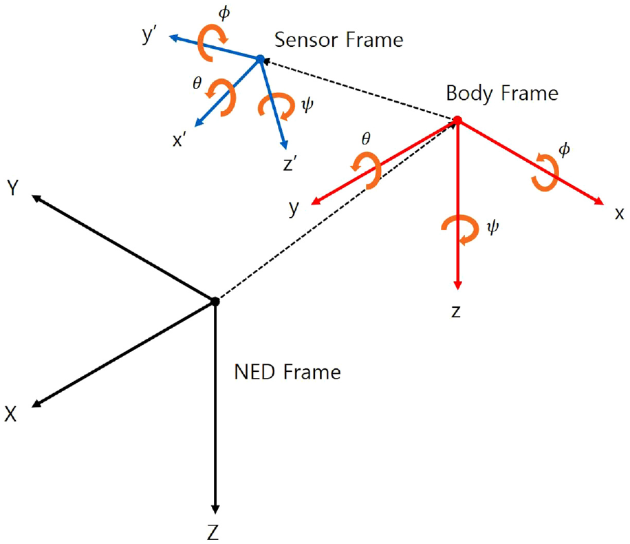
Coordinate systems involved in the study.
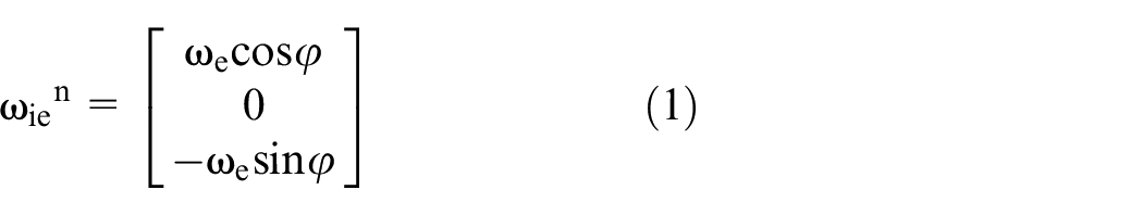
The inertial navigation system (INS) continuously calculates the posture change from the initial posture by using the angular velocity observation value of the gyroscope. 13 First, the angular velocity due to the rotation of the earth measured by the gyro sensor can be expressed by equation (1):
where
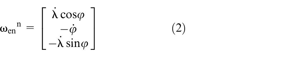
The angular velocity due to the motion of an object can be expressed by equation (2):
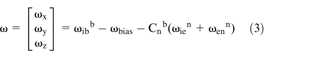
If the angular velocity of the body is calculated by removing the angular velocity component due to the rotation of the earth and the movement of the vehicle from the measured value of the gyro, it can be expressed by the following equation (3):
where
In this paper, the posture was calculated using the quaternion method, which has little error in posture change and does not cause gimbal lock. The composition of the quaternions is as shown in equation (4):

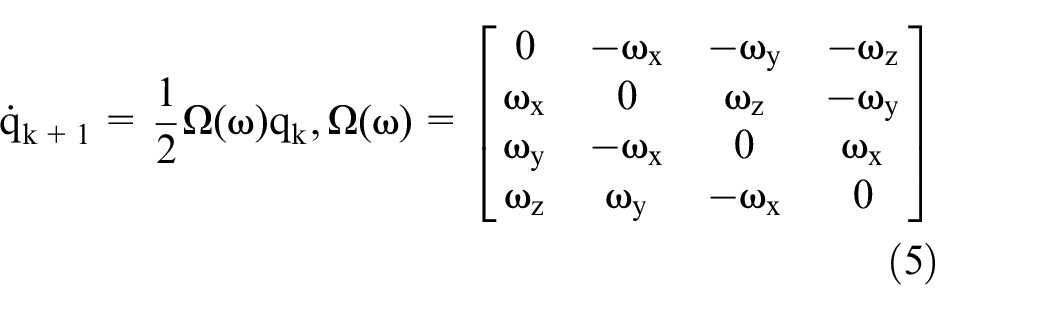
The quaternary differential equation to calculate the amount of change of posture from the calculated angular velocity of the body is as equation (5):
where
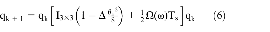
If the current posture of the quaternion is calculated using the calculated quaternary variance, it can be expressed by equation (6) 13 :
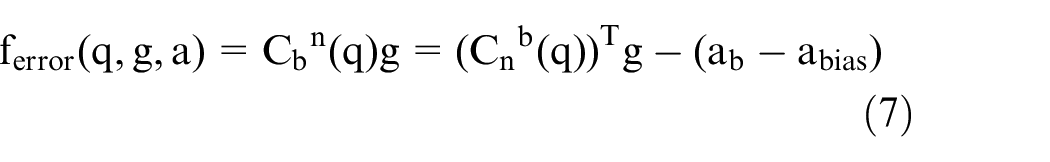
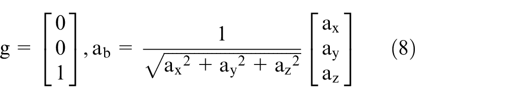
It is possible to calculate the gravity vector of the measured value from the current attitude, and the current roll and pitch angles can be known from the gravity vector. First, an error function is used to know the error that occurs when calculating the gravity vector from the accelerometer.
Equation (7) represents the error function:
where
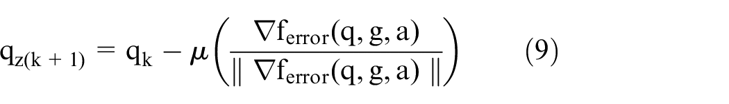
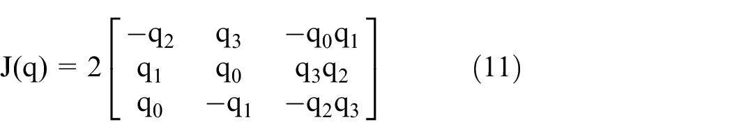
The gradient descent method is used to remove the quaternary error by using the acceleration error measured from the error function. The equation for removing the error of the current time from the posture of quaternion of the previous time can be expressed as the following equations (9)–(11):

The posture observation values of the two complementary sensors are fused using the Kalman filter. Figure 2 is the formula showing the structure of the Kalman filter that calculates the posture.
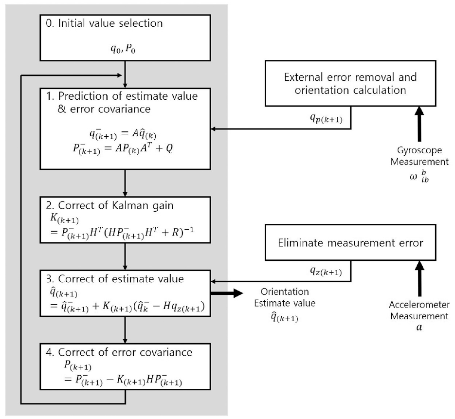
Kalman filter for orientation calculation.
The state variable estimated by the Kalman filter is set as the posture of the quaternion, and the measured value model
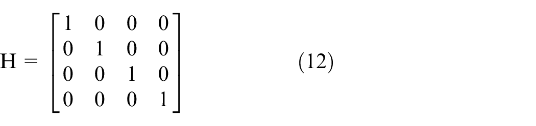
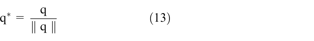
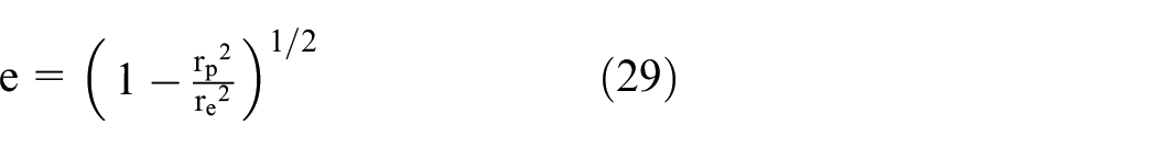
The state transition matrix and the covariance matrix for observation values were set as the error covariance of each posture observation value. In order to obtain numerical stability for the updated posture, a normalization process is performed as in equation (13):
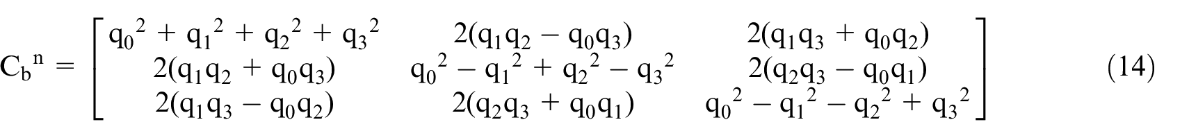
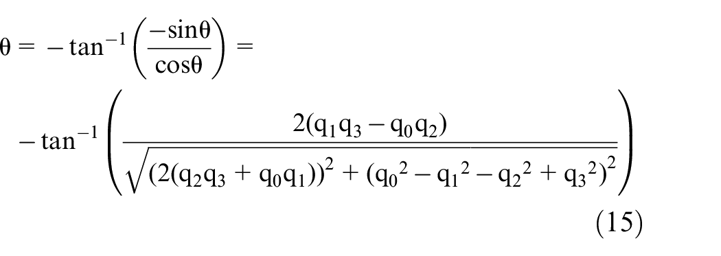
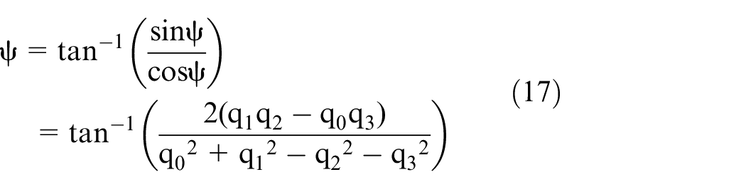
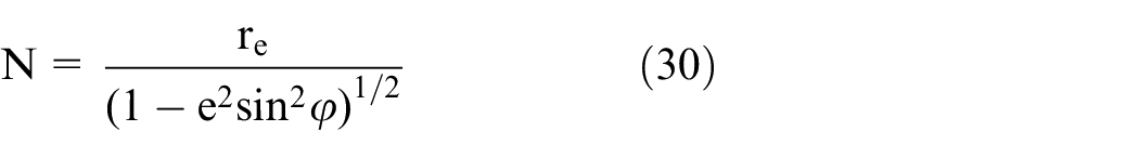
In order to calculate the current Euler posture and the coordinate transformation matrix from the finally calculated quaternions, it should be calculated using the coordinate transformation matrix as in equations (14)–(17):

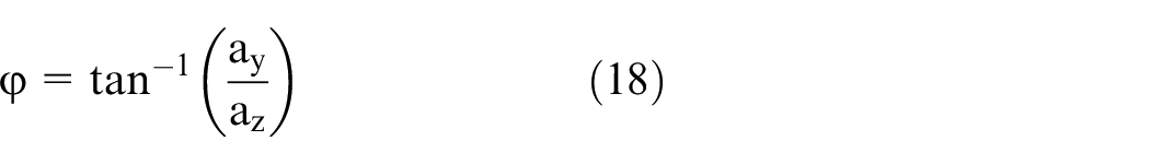
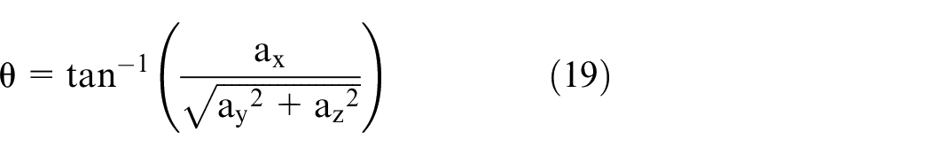
In order to obtain the posture of the moving body by inertial navigation, information on the initial posture of the moving body is required. In this paper, the initial posture was calculated using the coarse alignment method. At rest, acceleration has only the gravitational acceleration component. As shown in equations (18) and (19), since the direction of gravity always faces the ground, the initial posture for roll and pitch angles can be calculated from the direction of the gravity vector 14 :
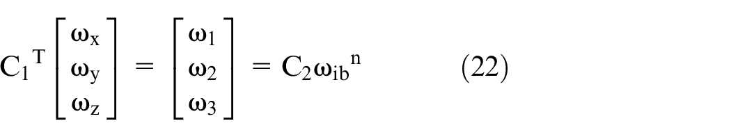
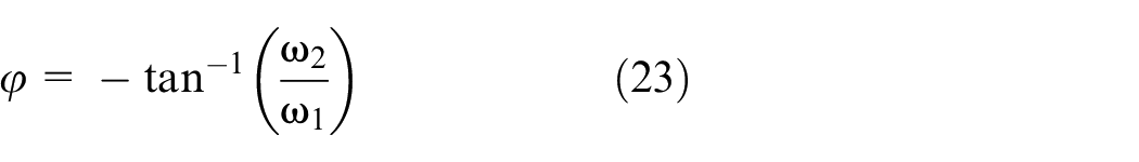
To calculate the yaw at rest, the angular velocity of the earth’s rotation is measured from the gyroscope. The earth’s rotation angular velocity


The component of
In INS, the velocity can be calculated as equation (24):

where
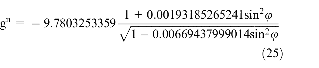
Since the accelerometer receives gravitational acceleration in the direction of the earth’s surface, it is necessary to measure the acceleration by removing the gravitational acceleration component to accurately measure the velocity. In order to know the gravitational acceleration according to the latitude, the gravitational acceleration of the vehicle is calculated from the gravitational model. 15 If the gravity model for the current gravity according to latitude is arranged by substituting earth-related variables, it can be expressed as equation (25):
A skew-symmetric matrix with respect to a three-dimensional vector
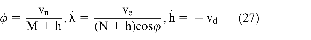
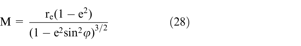
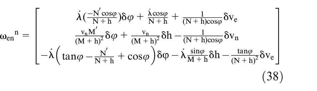
The movement of the vehicle moving near the ground surface can be obtained from the speed of each axis in the navigation coordinate system. If the amount of change with respect to the current latitude, longitude, and altitude is calculated from the velocity calculated above, it can be expressed as equation (27):
where
where
where
In INS, navigation errors occur due to errors in the sensors used for implementation, errors in the initial measured posture, and errors in calculations. In order to compensate for navigation errors, information about the errors is required.
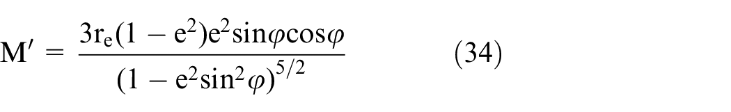
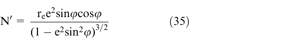
Equation (27), which is a differential equation for position change, can be expressed by differentially linearizing it with the Taylor series. Classifying the components of error in equation (27) can be divided into speed error, latitude error, altitude error, earth’s average radius of curvature error, and earth’s cross-sectional radius of curvature error. The results of error factors are summarized in equations (31)–(33) 16 :
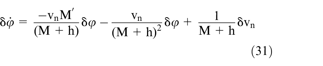
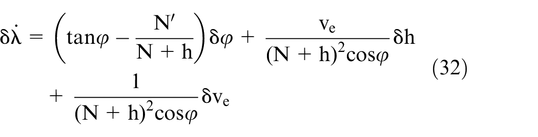

In equation (31),
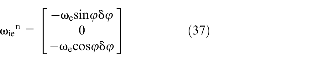
In the velocity calculation formula of equation (24), error factors can be divided into torsional error of current posture, bias error of acceleration measurement, error of angular velocity vector due to earth rotation vector and antibody motion, and velocity error. The velocity error model is shown in equation (36):
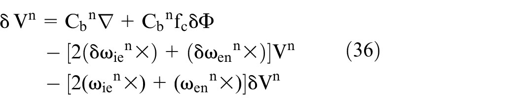
where ∇ is the random bias error of the accelerometer,
The posture error is in the form of a differential equation of the torsional error generated from the reference posture, and can be expressed by equation (39):
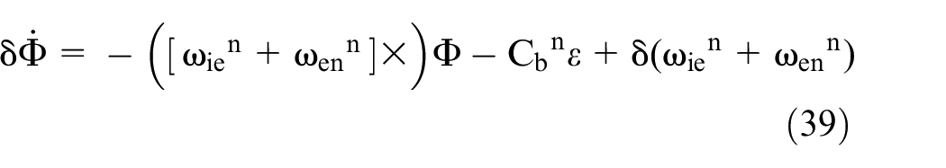
The error between the accelerometer and the gyro is an irregular error and can be expressed by equations (40) and (41):


where ∇ is the random bias error of the accelerometer,
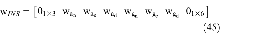
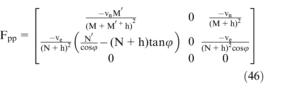
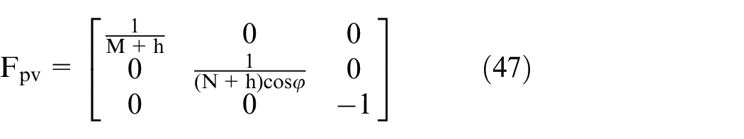
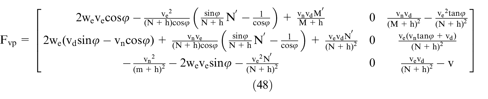
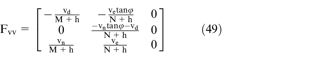
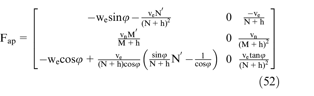
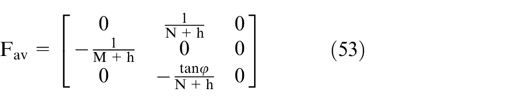
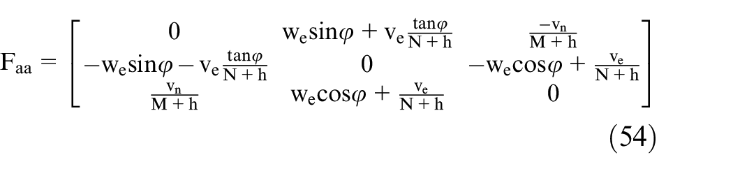
The system model uses the error model of the INS.7,17 The EKF is used to fuse the INS and the GPS. The state variable is estimated by the Kalman filter is as shown in equation (42) 18 :

where
The equations of state of the Kalman filter are as shown in equations (43) and (44) 7 :

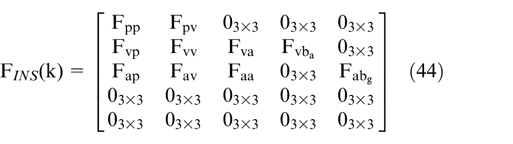
The process noise


In this study, the GPS measurement was determined as an outlier if the following two conditions were satisfied
12
: the difference between the position (

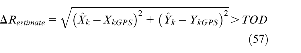
where
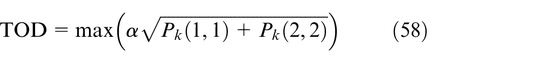
where
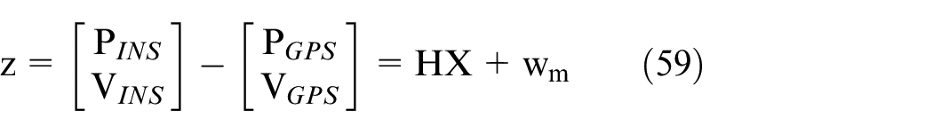
The measurement errors of the two navigation systems in a loosely coupled method can be calculated based on the difference in position and velocity data. Here,

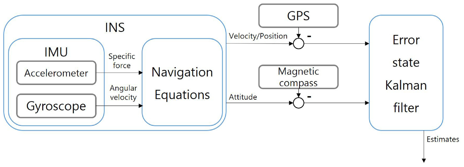
A block diagram of the proposed navigation algorithm is shown in Figure 3. As mentioned above, the INS is configured through the IMU, where the velocity and position deduced from the INS are calibrated using GPS, while the direction angle is calibrated using a magnetic compass. Finally, the final outputs (velocity, position, and direction angle) were deduced using the EKF.
Block diagram of the navigation system.
Simulation results
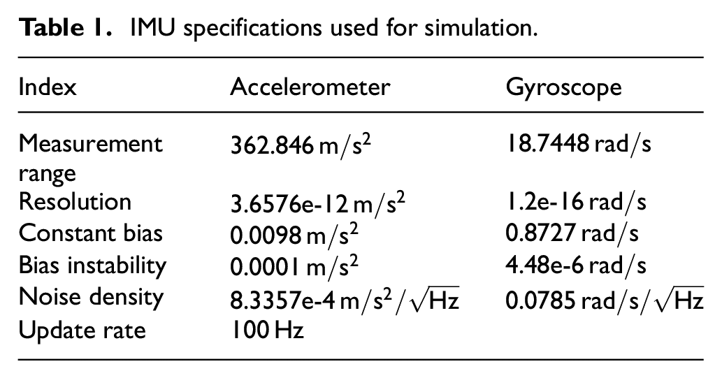
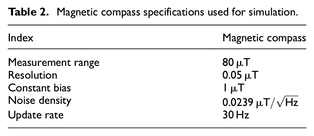
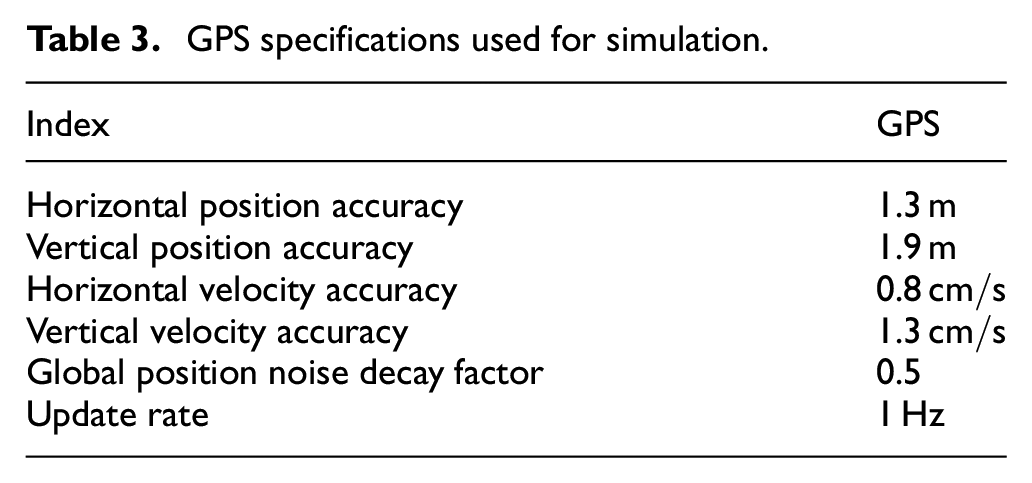
A simulation was performed to examine the performance of the system before conducting an experiment on navigation. The sensors used in the simulation include an accelerometer and a gyroscope of the IMU, magnetic compass, and GPS. Table 1 lists the major parameters of the IMU, Table 2 lists the major parameters of the magnetic compass, and Table 3 lists the major parameters of the GPS used in the simulation. The parameters of all the sensors were selected based on the specifications of the sensors used in the navigation system developed in this study.
IMU specifications used for simulation.
Magnetic compass specifications used for simulation.
GPS specifications used for simulation.
First, the simulation inputs such as acceleration, angular velocity, and direction angle of a vehicle based on which a path the vehicle moves were generated for comparison with the navigation results. Second, measurements were generated by inputting acceleration, angular velocity, and direction angle to the sensor using the IMU model. 13 Third, the GPS position data were generated by utilizing the moving path generated by the GPS model as an input. The final outputs (position, velocity, and direction angle) were deduced based on the data of the accelerometer, gyroscope, magnetic compass, and GPS generated previously using the navigation method explained above.
Figure 4 shows the sensor measurements resulting from the angular velocity, acceleration, and direction angle generated by the IMU model as inputs. Measurements of the sensors were computed according to the parameters of each sensor in which the gravitational component was added in the z-axis direction for acceleration, while noise was added to the sensors.
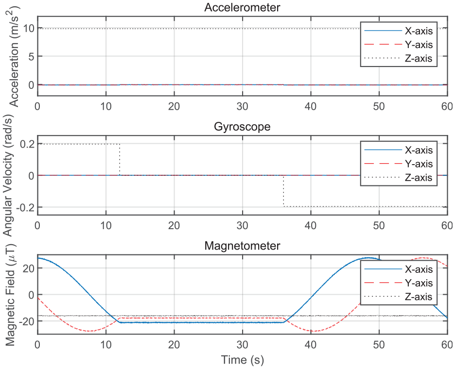
Sensor data generated using the IMU model.
The position results of the navigation are shown in Figure 5. The initial position is [0 0 0] m, and the final position after two rotations is [0 90 0] m. The trajectory is a position reference value that indicates the moving path of a vehicle that has been generated previously. GPS is the position measurement generated from the GPS model based on the position reference value as an input. The estimate shows the position result of the navigation. Navigation finds the direction angle at 100 Hz using an accelerometer and gyroscope and at 30 Hz using the position, velocity, and magnetic compass. The position and velocity data were calibrated to 1 Hz using the EKF. Therefore, the result of navigation does not have a significant error, even if the GPS position data has a large error, as shown in Figure 5. Figure 6 shows the direction angle of the navigation, which is similar to the actual direction angle.
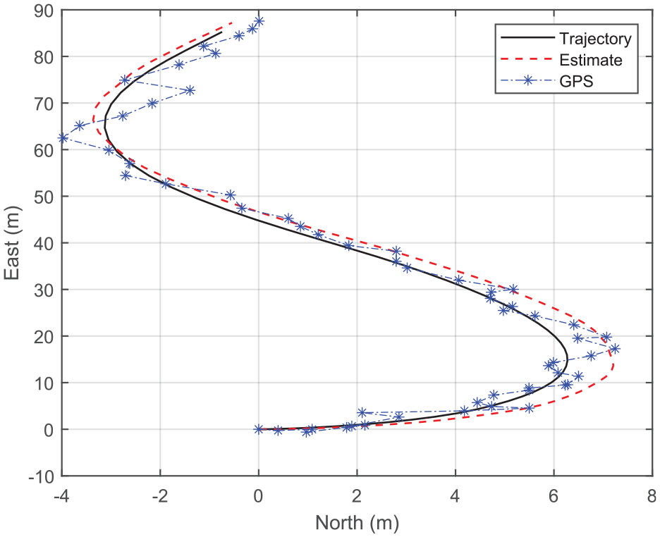
Position of navigation.
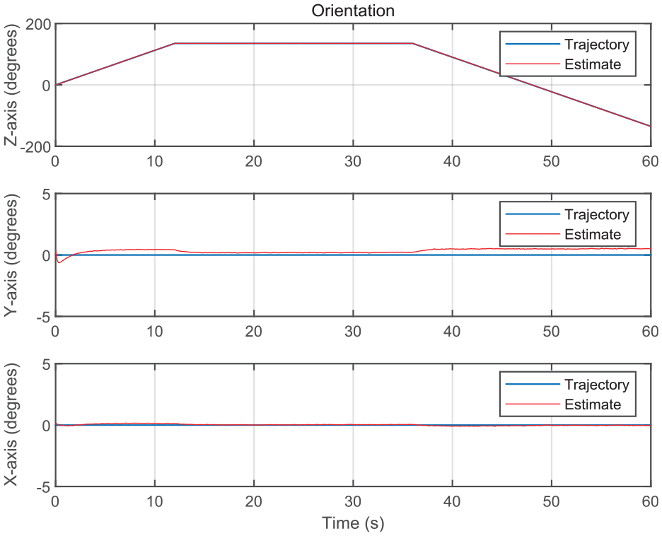
Orientation of navigation versus trajectory.
The velocity results of the navigation are shown in Figure 7. Real shows the moving velocity of the actual vehicle calculated using the accelerometer, while estimate shows the velocity of navigation. The velocity of the accelerometer was integrated once for the representation. Because the velocity result of navigation is calibrated at 1 Hz through GPS data, the velocity changes according to the update rate, as shown in the graph. Figure 7 shows that the velocity result of the navigation is adequately estimated.
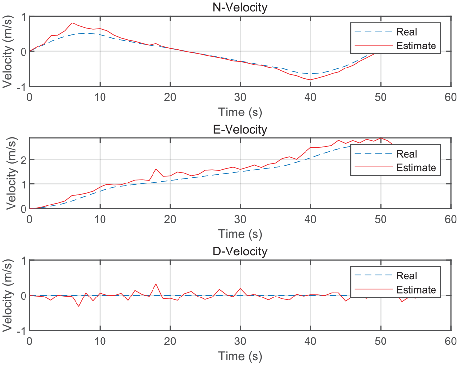
Each velocity of navigation.
Figure 8 shows a comparison between the position result of navigation and the actual position. For each axis, the trajectory shows the actual position, whereas the estimate shows the position information of navigation. The greatest error of each axis was −1.4 m for the x-axis, –2 m for the y-axis, and 1.2 m for the z-axis; the root mean square (RMS) error of the position was [0.7 1.46 0.71] m.
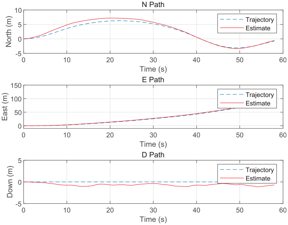
Position of navigation versus trajectory.
Experiments and results
System configuration
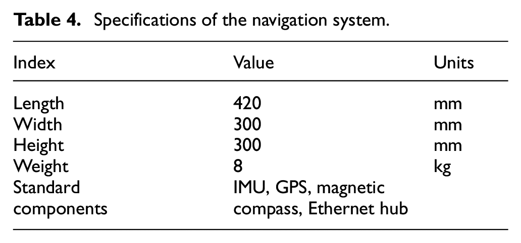
To verify the performance of the navigation algorithm proposed in this study, the navigation system shown in Figure 9 was developed. Using an aluminum box shape, a GPS antenna was mounted at the top. The system was equipped with sensors for navigation, an Ethernet hub for communications, and an interface board for providing power for sensors and data communications. Table 4 presents the specifications and devices used in the navigation system. The IMU, GPS, and magnetic compass were used as sensors in the navigation system. A ring laser gyroscope (RLG) was selected as the IMU to improve the computation performance of the INS.
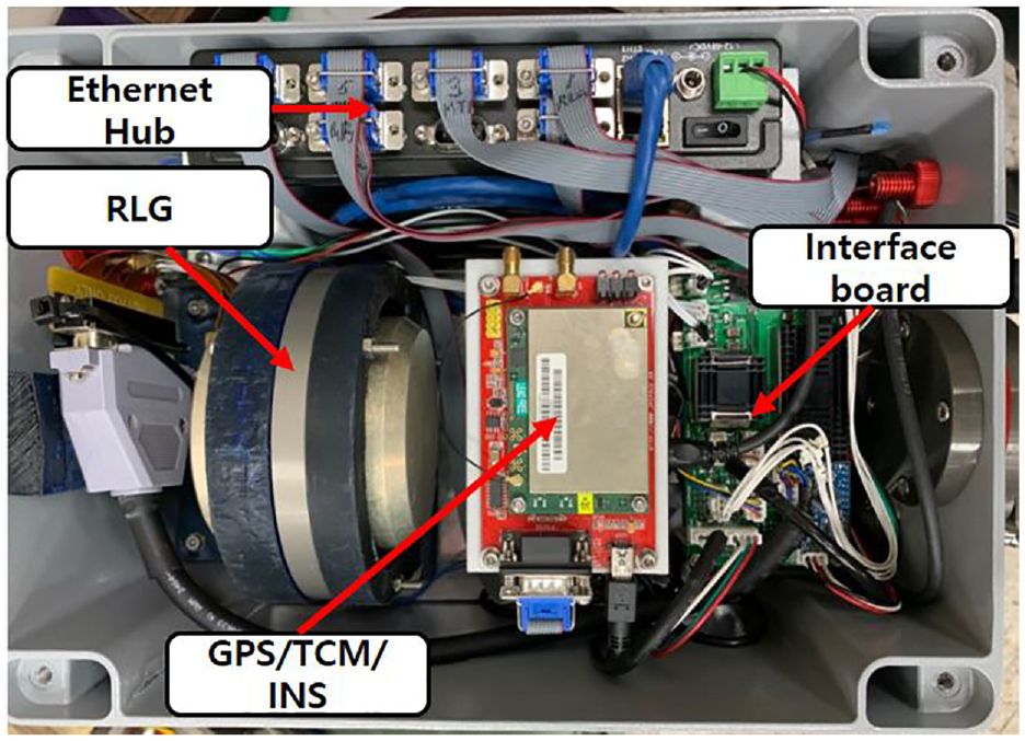
Developed navigation system.
Specifications of the navigation system.
Performance experiment
The basic performance of the navigation system was verified before conducting the experiment. The navigation system was moved eastward by 20 m to measure the position of the vehicle, and the measurement results were compared with the navigation system results. At this time, as I was moving on the road using a vehicle, it was not possible to move in a straight line in the east direction. In Figure 10, the GPS result represents the GPS measured position (star-dotted line), navigation result represents the proposed navigation estimated position (red solid line), DR represents the position estimated by DR (solid dotted line), and trajectory represents the actual position (black solid line).
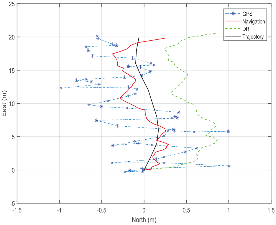
Positions of trajectory and navigation.
The experimental results in Figure 10 show that the estimated position of the proposed navigation is similar to the actual position but varies slightly from the position estimated by DR. The measured position of the GPS acquired during the experiment showed that a large error was produced owing to the horizontal precision of the vehicle. The experimental results showed that the proposed navigation position result is most similar to the actual position compared to other navigation results.
Figure 11 highlights the error between the actual position and the proposed navigation position. The north axis is represented with a + symbol, while the east axis is represented by an * symbol. The comparison results show that the maximum error for each axis is [0.267 0.5503] m, and the RMS error is [0.13 0.22] m. The experiment proved that the proposed navigation system estimates the position within an RMS error of 0.3 m.
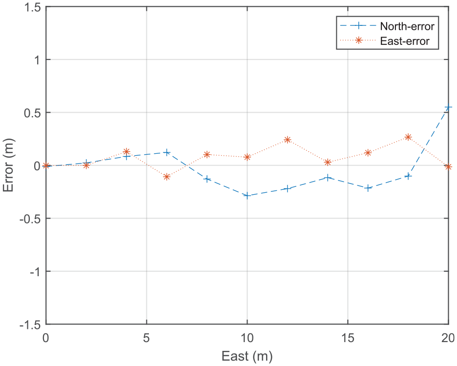
The error between positions of trajectory and navigation.
Navigation experiment
The navigation performance experiment was conducted by moving the developed navigation system along a horizontal trajectory. The navigation performance was tested on land using a navigation system and a small vehicle. In order to increase the GPS reception sensitivity, an experiment was conducted in a playground with no tall buildings nearby. In Figure 12, the estimated position of the proposed navigation algorithm is shown in terms of a horizontal trajectory in which GPS represents the measured position of the GPS (dotted line), while the navigation represents the estimated position of the proposed navigation (solid line). The vehicle started from the [0 0] m, moved counterclockwise in a distorted square trajectory, and stopped at the [0 –6] m. The results showed that the estimated navigation position was similar to the GPS measured position; the data near the point ([–16 −7.5] m) showed vibrating patterns, possibly due to the vibration that occurred when the vehicle moved from a polyurethane track to grass. The proposed navigation system removed the outliers to estimate the position even when outliers occurred in the GPS position during the experiment. Figure 13 shows the difference between the GPS measured position and the estimated navigation position for each axis; the largest error of each axis is 2 m for both the x-axis and y-axis, and the RMS error of the position is [1.18 0.94] m.
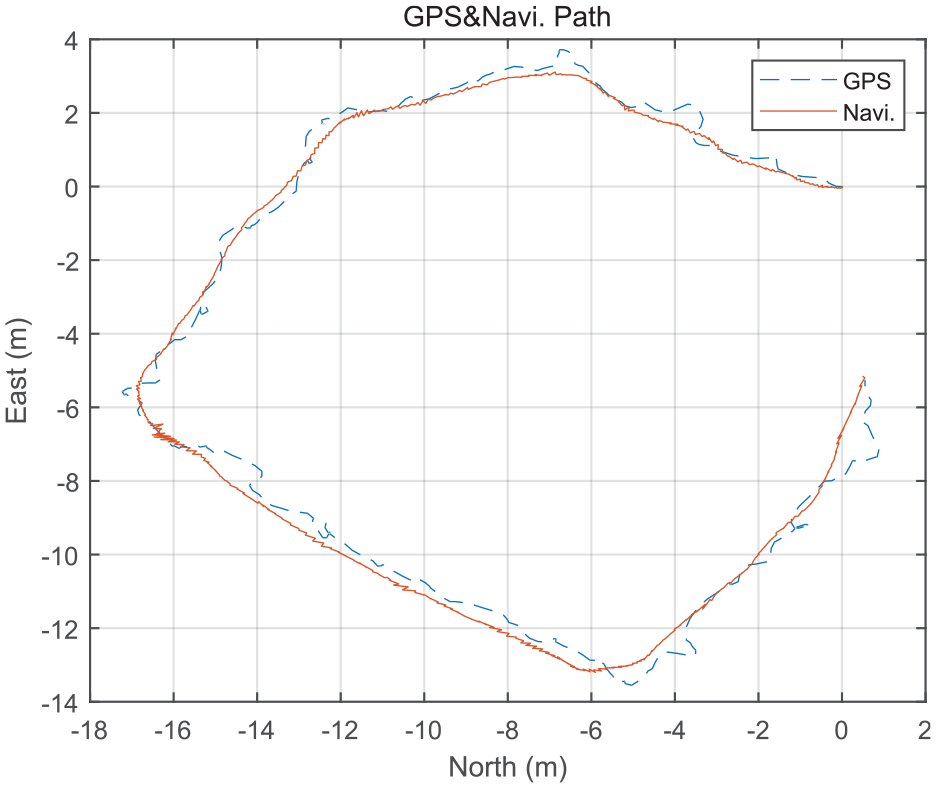
Position of navigation.
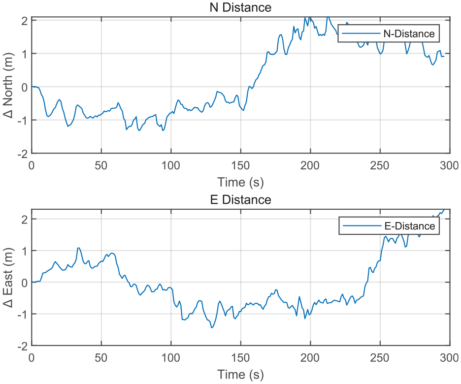
Difference between the position of navigation and GPS.
Figure 14 shows the velocity component estimated using the proposed navigation system. The results show that the maximum velocity in each direction is [0.6 0.3] m/s, while the mean velocity is [–0.05 −0.01] m/s. At approximately 180 s, the velocity in the x-axis abruptly changes by ±0.6 m/s, which is presumed to be the vibration generated when the vehicle moves from a polyurethane track to grass. The results confirmed the difference between the height of the polyurethane track and grass in which the polyurethane track is positioned higher than the grass. The velocity was estimated well even when the navigation system vibrated substantially owing to the ground state.
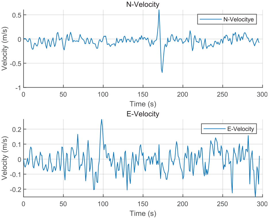
Velocity of navigation.
Figure 15 shows the angular components estimated by the proposed navigation system. Previous experimental results showed that the progression direction changed considerably at approximately 70, 150, and 240 s. Moreover, the heading and pitch instantaneously changed at 180 s as the vehicle moved from a polyurethane track to grass, as explained earlier.
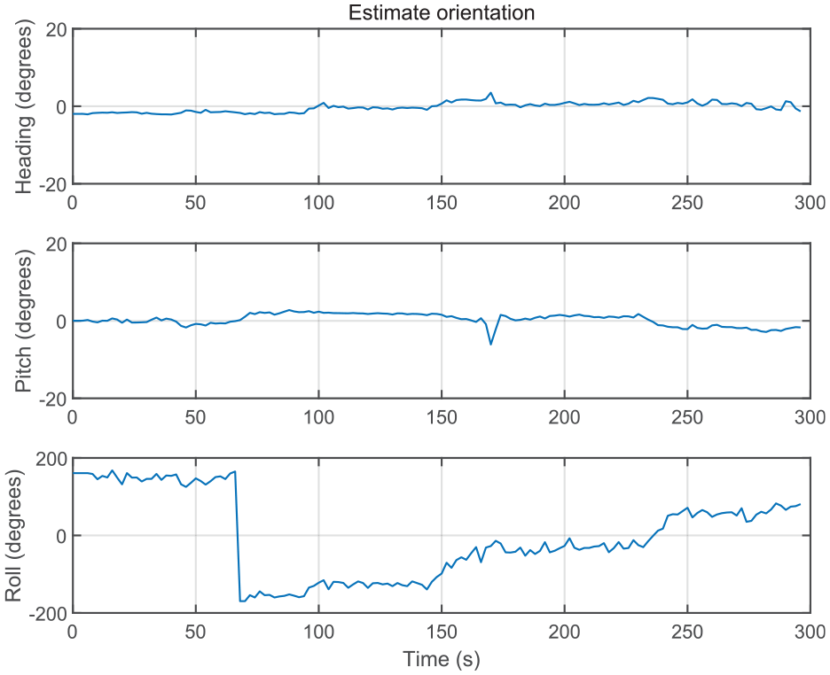
Orientation of navigation.
Conclusions
Extensive research is ongoing on autonomous exploration and operation which requires navigation. DR, which is a general type of navigation, has limited estimation within a short period of time. Therefore, integrated navigation using auxiliary navigation sensors is required. However, a technique for detecting and removing outliers is required owing to the presence of navigation sensors that generate outliers. Therefore, in this study, a navigation algorithm with a technique for removing outliers of GPS was designed to develop a navigation system. Furthermore, an experiment was conducted using the developed navigation system to verify the effectiveness of the proposed navigation algorithm.
First, the INS was configured through the IMU, where the velocity and position deduced from the INS were calibrated using GPS, while the direction angle was calibrated using a magnetic compass. Finally, the final outputs (velocity, position, and direction angle) were deduced using EKF. A simulation was also performed before conducting the experiment on the proposed navigation algorithm. The parameters of all the sensors used in the simulation were selected based on the specifications of the sensors used in the navigation system developed in this study. The simulation confirmed that the navigation system effectively estimated the position.
A navigation system was developed to conduct an experiment to verify the performance of the proposed navigation algorithm, which was tested as follows. The experimental conditions were ground surfaces of the polyurethane track and grass. The first experiment result showed that the RMS error (compared to the actual position) of the navigation system was within 0.3 m; the second experiment on the navigation performance showed that the proposed navigation estimated the position more effectively than the conventional navigation method, DR. Even when outliers occurred in the GPS position during the experiment, the proposed navigation system removed the outliers to estimate the position.
Previous experimental results showed that the position data measured in real-time from the GPS, used for calibrating the position, a large amount of noise, whereas the position data collected by the proposed navigation algorithm included much less noise. The proposed navigation estimated the velocity more effectively, thus reducing the error in position estimation, which is the final output. This paper presents a simple and inexpensive navigation system. With these advantages, the performance can show a degree similar to that of the systems already on the market.
Footnotes
Declaration of conflicting interests
The author(s) declared no potential conflicts of interest with respect to the research, authorship, and/or publication of this article.
Funding
The author(s) disclosed receipt of the following financial support for the research, authorship, and/or publication of this article: This research was supported by the Unmanned Vehicles Core Technology Research and Development Program through the National Research Foundation of Korea (NRF) and Unmanned Vehicle Advanced Research Center (UVARC) funded by the Ministry of Science and ICT, Republic of Korea (NRF-2020M3C1C1A02086324).