Sage Journals: Discover world-class research

Abstract

Evolutionary Algorithms (EAs) are routinely applied to solve a large set of optimization problems. Traditionally, their performance in solving those problems is analyzed using the fitness quality and computing time, and the effect of evolutionary operators on both metrics is routinely used to compare different versions of EAs. Nevertheless, scientists face nowadays the challenge of considering the energy efficiency in addition to computational time, which requires studying the energy consumption of algorithms.

This paper discusses the interest of introducing power consumption as a new metric to analyze the performance of standard genetic programming (GP). Two well-studied benchmark problems are addressed on three different computing platforms, and two different approaches to measure the power consumption have been tested.

Analyzing the population size, the results demonstrates its influence on the energy consumed: a non-linear relationship was found between size and energy required to complete an experiment. This analysis was extended to the cache memory and results show an exponential growth in the number of cache misses as the population size increases, which affects the energy consumed. This study shows that not only computing time or solution quality must be analyzed, but also the energy required to find a solution.

Summarizing, this paper shows that when GP is applied, specific considerations on how to select parameter values must be taken into account if the goal is to obtain solutions while searching for energy efficiency. Although the study has been performed using GP, we foresee that it could be similarly extended to EAs.

Keywords

energy consumption evolutionary algorithms energy-aware computing performance measurements

Introduction

Energy efficiency has acquired a remarkable importance in the last decades for the scientific community, due to the growing need of information and communication technologies and therefore power-operated systems in society.¹

In recent years, attention has been paid on the management of the power consumption on the whole field of Information Technology (IT), from the circuit level—which includes microprocessors, network-based systems, hand-held devices, etc.

Regarding microprocessors, the most successful technique, the Dynamic Voltage and Frequency Scaling (DVFS) is widely spread in available computer architectures. DVFS, initially aimed at single processors, saves energy by switching the processor’s frequency and voltage according to the workload needs. Relying on this technique, many algorithms have been developed,^2–4 also to minimize energy consumption of a real time parallel application with precedence-constrained tasks on a heterogeneous distributed system.⁵

Multiple approaches have addressed the cache memory in order to save energy. Hu et al.⁶ for instance, proposed a feedback mechanism to perform the data cache resizing. This approach blocks the low yields of cache resizing using the information of the cache footprint, improving the cache performance and saving 10% energy, compared with the cache without the feedback mechanism. Manohar et al.⁷ presented a value-based refresh saving method for Muti-level cache hierarchy with large sized last level caches (LLCs). The aim is minimizing the number of refreshes and save energy when embedded-DRAMs (eDRAM) are used as an alternative to SRAM.

These techniques are directly applicable to different hardware components configuration. Nevertheless, power consumption can also be studied from the algorithm point of view, where optimizations can also be applied. Our approach is focused on this level, particularly the algorithms settings.

If we focus on this area, we found several works that study algorithms considering energy consumption point of view. Mota et al.⁸ tackled a comparative analysis, where commonly used symmetric and asymmetric encryption algorithms are analyzed using several metrics, including efficiency in terms of power consumption. Kong et al.⁹ presented a routing protocol based on genetic algorithm to construct an energy-aware middle layer oriented network. The schemes proposed consume less energy when compared to other methods, and they also extend the network lifetime.

More recently, Rashid et al. measured in Ref. 10 the power consumption of several sorting algorithms. In that work, the algorithms were coded in different languages and were run on an ARM architecture and the key factors affecting energy consumption were identified. Same authors in Ref. 11 analyzed the power consumption of common image encoding and decoding algorithms such as JPEG and PNG on an ARM platform. They found JPEG consumes up to 37% more energy than PNG.

As described above, a number of algorithms have already been analyzed from the point of view of power consumption. But in the case of EAs, this idea has only been presented in the literature very recently, and still needs development as Camacho et al. described in Ref. 12. Recently, Talbi et al.¹³ proposed a unified view to guide the design and implementation of efficient and effective parallel evolutionary algorithms for multi-objective optimization, where the energy consumption of the MOEA itself is proposed to be considered as a metric.

As we show below, few authors have ever considered that power consumption must be studied in the case of EAs, and the possible influence of the parameter values on the energy efficiency of the algorithm has never been studied. In this paper, we pursue that goal: to analyze the influence of population size on Genetic Programming (GP) power consumption. To the best of our knowledge, this is the first systematic study of such an issue. Thus, the main contribution of this paper is to show that energy consumption is not directly related to runtime for GP. Moreover, we show the relationship between population size and energy consumed, describe some anomalies detected and look for the reasons behind that behavior.

Our results demonstrate the influence of the population size on the energy consumed: a non-linear relationship was found between size and energy required to complete an experiment. The extension of the study to the cache memory shows an exponential growth in the number of cache misses as the population size increases, which affects the energy consumed. Therefore, our study results contribute to confirm that not only computing time or solution quality must be analyzed, but also the energy required to find a solution. We thus hope this paper will pave the way towards energy efficiency of GP and EAs in the future.

The rest of the paper is organized as follows: in Power Consumption and EAs we describe previous approaches in the area, the motivation for this analysis and the outlines of this study are presented. Methodology describes the methodology for the analysis and the benchmark problems selected. Results presents the results obtained, and finally Conclusion draws our conclusions and future work.

Power consumption and EAs

From a historic perspective, EA researchers have always considered the quality of solutions found and computing time required to find them as the most important metrics to evaluate the performance of the algorithm, while the energy consumption has usually been ignored. In regard of the computing time, it seems to be accepted that the relationship between the power consumption and runtime is linear, and the processor’s instantaneous energy consumption is constant, whatever the operation performed by the CPU. Thus, the power consumption could be easily calculated by multiplying the instantaneous consumption of energy, at any time during the experiment, by the total execution time. This assumption has probably kept researchers from considering energy consumption as something that deserves attention. But this is certainly not the case, as has already been shown when the power consumption is analyzed from the point of view of computer architectures.¹⁴

Moreover, in a previous and preliminary research work, we detected some anomalies related to the parameter values employed when running the algorithm.¹⁵

Although the relationship between power consumption and EAs is not new, the literature frequently describes works where the role of the EA is the standard one, an optimization method, and power consumption is simply the goal to be optimized in a given context. A proper review of this idea can be found in Refs. 16, 17. In Ref. 18, for instance, researchers proposed a Genetic Algorithm (GA) to improve the warehouses energy management to minimize the impact on the environment and to reduce the associated costs.

On the other hand, Liqat et al. developed in Ref. 19 a scheduling tool in charge of dividing a program into basic blocks; then an EA is applied to establish the maximum limit of energy for each block. Recently Ibrahim et al.²⁰ presented an adaptive GA to search the optimal scheduling solution to minimize the power consumption in a cloud computing infrastructure.

A recent study²¹ performed a systematic study of the energy complexity of several classic algorithms exploring the time/space/energy trade-off in order to reduce their energy complexity by applying Landauer’s principle.

Similarly, as in the previous works, we share the quest for energy-efficient algorithms as the main goal. Nevertheless, some differences can be drawn. Our study is applied to GP, while above-mentioned work deals with several classical algorithms. We study some parameter values that affect the algorithm behavior, while they focus on a lower level, particularly on word-level operations, and build pseudo-code for well-known and new programming structures, both in terms of control logic, memory allocation, garbage collection, logging, and unrolling operations.

Therefore, our point of view is quite different since we focus on studying the optimal parameter values for EAs, particularly GP in this work, to achieve a trade-off between quality of solutions and energy consumption.

Closer to our goals, García-Martín et al.²² presented a general literature review of different methods and power models to estimate power consumption in machine learning applications. Additionally, they presented the latest software tools available to estimate power consumption in this context. Some of the methods reviewed are applied in this work, as we describe below, although we also include additional measurement procedures, as we describe below.

To the best of our knowledge, few research works deal with the problem of quantifying the energy required by evolutionary algorithms when tackling a real-world problem optimization. Closely related to that idea, Abdelhafez et al.²³ compared a sequential and a parallel genetic algorithm in terms of the power consumption. Regarding the parallel GA approach, authors analyzed both the synchronous and asynchronous version of the algorithm. They worked with a different number of cores and dimensions for several problems and focused on crossover and mutation operators. Lately, several works were presented related to this goal.

Population and chromosome size were studied for the first time in Ref. 15, where the energy consumption patterns where analyzed using two well-known benchmarks of a simple GA. However, this analysis did not include GP.

Power consumption in genetic programming

The work presented here improves on some aspects of the previous work, allowing us to draw useful conclusions. First of all, the benchmark problems must be carefully selected, as described in Ref. 24. On the other hand, we should focus on the main parameters of the GP, and their influence on its energy footprint. Furthermore, this should be contextualized in relation to standard metrics, such as fitness quality and computation time.

In terms of the benchmark issues to be tested, the GP community identified some issues over the last decade,²⁴ which were related to the quality of the traditionally employed GP benchmarks. In that work, the authors warned of the need to design a good benchmark suite. In this context, McDermott et al.²⁵ proposed a new set of GP benchmarks as better candidates for testing GP. With this in mind, we have selected two of them to work with, namely Lid and Order Tree.

Lid is a GP benchmark, which can adjust its difficulty by changing maximum individual sizes and depths allowed. Order tree is a new GP benchmark that shares properties with other GP benchmarks and solves some shortcomings. The problem size and the linearity of the fitness structure can be increased and decreased, respectively, to tune the difficulty of the problem. In this paper, we focus on the population size and the rest of the alternatives will be addressed later.

Based on the foregoing, in this paper, we consider the standard version of GP to be run on selected benchmark problems, and we decided to explore the influence of population size as one of its main parameters.

The standard operations of the algorithm, fitness evaluation, selection, crossover, and mutation are repeated in each generation. But from the point of view of the CPU, running the algorithm, there are no major differences when CPU time is devoted to running the algorithm, although perhaps other issues may affect the energy consumed, such as cache memory operations, as we study below.

In a previous work, we focused on a preliminary analysis of the algorithm, taking into account the hardware platform on which it can be run (see Ref. 26). As a result, a profile was generated for each platform that was then analyzed in Ref. 27. A preliminary study limited to the 6-bit multiplexer GP problem was conducted using small population sizes. Nevertheless, that work was aimed at studying the most energy-efficient platform, and the goal is now quite different. All in all, those results suggest that the idea is worth pursuing further.

When we look at the number of generations and population size, as well as the running time of the algorithm, computing N + 1 generations will take longer than N; evaluating a population size of I + 1 individuals will take longer than I. In addition, a more complex fitness function needs more time to evaluate each individual and, consequently, the runtime grows. Similarly, a greater depth of the trees increases the difficulty of the problem and, consequently, the computing resources required. Therefore, the study of the influence of different parameter values is crucial for the analysis of energy consumption behavior.

In this work, we consider two different perspectives to analyze the energy consumption behavior for each GP benchmark: (i) Running the algorithm for a given time without taking into account the quality of the solution found and (ii) Running the algorithm until a given quality solution or number of generations is reached. Both perspectives coincide with those proposed when considering real-world problems.

We believe it is important to evaluate the influence of the main parameters on the energy required to run an EA, and to make decisions based on finding a compromise between solution quality, execution time and energy efficiency.

In the following section, we describe the methodology applied to study the energy consumption of the GP. Three different computing platforms have been used and two different approaches have been applied to measure as accurately as possible the energy consumption. Our main goal here is to provide evidence on the importance of parameter selection if we want to achieve energy efficiency in the future for EAs; we also try to show that there is no linear relationship between computing time and energy consumption, and therefore studies like the one we present deserve attention. To the best of our knowledge, this is the first time this relationship has been studied with the precision described here.

Methodology

This work is based on the hypothesis that the main EA parameters not only influences computing time or quality of solutions, but they highly influence the total energy consumed by the algorithm when addressing a problem. Moreover, previous work has shown that correlation between time and energy, that is assumed as a direct one, seems to be not so direct and deserves attention. Therefore, this study focuses particularly on this issue, specifically applied to GP. In this light, an appropriate selection of parameter values could further provide more energy-efficient algorithms.

We have thus selected and studied the population size as one of the most influencing parameters and tackled the two GP benchmarks previously described: LID and ORDER Tree. The main objective is measuring accurately the energy consumption for a set of population size values and analyzing results obtained.

Our experiments were carried out on three different computer platforms, which provide different computational resources. We consider that the use of multiple platforms allows the results to be extrapolated to any other hardware platforms. The first one was a Raspberry Pi 3 Model B+,¹ which is a Single-board computer equipped with a Quad Core 1.2GHz Broadcom BCM2837 64bit CPU 1GB RAM and connectivity with a BCM43438 wireless LAN and Bluetooth Low Energy (BLE) on board. The operating system was Raspbian 7. Raspberry Pi has been widely used as the target platform in many optimization process, some very recently.^28,29 The second platform was an ASUS Laptop with a processor Intel(R) Core(TM) i5-2450M 2.5 GHz, 4 cores and 8GB RAM and Ubuntu 14.04.1 LTS as the operating system. Finally, we also ran our experiments on a desktop personal computer (PC) provided with an Intel(R) Core^TM i5-4430 processor, 3 GHz, 4 cores, 32GB RAM using as operating system Ubuntu 14.04.1 LTS.

The reason for including the Raspberry Pi platform is due to previously published results describing it as the most energy-efficient platform for running an EA.²⁶

Once the target platforms were selected, we needed to choose the measurement system to quantify the energy consumption of the algorithm. We decided to use two different methodologies. On the one hand, we measured the power consumption on the Raspberry Pi and Laptop platforms with a professional digital power meter. On the other hand, we used a software tool for measuring the power consumption on the PC platform taking advantage of the specific registers of the CPU. This decision was taken as the PC is integrated into a rack at another research center, making it impossible to install the professional digital power meter to obtain the energy consumption data.

The following elements composes the instrumentation tools used to measure the energy consumption:

• A digital power meter, particularly the WT310E model from Yokogawa,³⁰ which is a power measurement instrument that can measure parameters such as voltage, current, and power at customized regular intervals (between 100ms to 20s), when running the algorithm on the target platforms, Laptop and Raspberry Pi in this case. Moreover, it provides of the WTViewer software application to save the samples taken in a complete log for further analysis and visualizing.

• The APPPowerMeter² software application, which is a powerful tool for monitoring CPU power with Intel’s RAPL interface.^31–34 AppPowerMeter monitors an application and takes samples of the CPU every 100ms. Thus, it is able of measuring the total energy and average power of the CPU while an application is run.

As previously mentioned, two well-known GP benchmark problems were chosen for this study: LID and ORDER Tree problems. The evolutionary engine ECJ^35,36 was used to carry out the experiments. All experiments used ECJ’s default values for evolutionary parameters. Particularly, probabilities of crossover and mutation equal to 0.9 and 0.1, respectively. The trees initialization method applied was ramped half-and-half. The number of generations is selected large enough to exceed 300 s and population size corresponds to the customized settings of each experiment. We must bear in mind that a run will finish always after a given number of generations is completed, or when the running time is longer that 300 s.

Six different population size values were tested, 256, 512, 1024, 2048, 4096, and 8192. Once the specific parameters settings are established, the generational version of the algorithm is launched (30 independent runs for each population size). As a result, the average values are obtained. The setup establishes that each independent run will finish when exceeding 300 s (maximum time allowed per run), which may correspond to different number of generations computed, given variable individual size that GP features.

In order to gather results and energy consumption data, a differentiation needs to be made between the experiments carried out on the PC platform, and those on the Laptop and Raspberry Pi platforms. Both collect evolutionary information from the evolutionary engine ECJ, which provides a log with evolutionary data such as the best fitness value for each generation. This log was enlarged to add the total system time to complete each generation. However, the measurement of the energy consumed is carried out of the tool, using two different approaches. When the PC platform is employed, we use the AppPowerMeter software, which receives as an argument the application to be executed and when finishing it returns the average total energy consumed, power, and time, obtained from the registers of the CPU via the Intel’s RAPL interface. The idea behind the use of different methods to monitor the energy consumption allows us to evaluate the reliability of the results.

The energy consumed running the experiments on the Laptop and Raspberry Pi platforms is measured using the digital power meter and the WTViewer software application, which stores all samples taken during the algorithm run into a log file. This information is further processed for obtaining the energy consumed. Results obtained are summarized and analyzed in the following section.

Results

Three different experiment settings, detailed in the next subsections, have been designed, that are summarized as follows:

• Experiment #1: Running experiments for 300 s, and analyzing energy consumption for every population size considered.

• Experiment #2: Running experiments until solutions with a given fitness values are found.

• Further Experiments: The conclusions reached in the previous stages led us to conduct further experiments that may shed light into results and behaviors found.

Experiments with time limit 300 s

The initial experiment aims at evaluating all benchmark problems on hardware platforms and testing all population sizes selected. Thus, 30 independent runs were launched and each run was stopped when a given generation ends and the running time overpass 300 s, which is the maximum allowed time. Therefore, time monitoring is performed just after each generation is completed. Given that some runs will for sure exceed the limit of 300 s, two types of graphs are shown for this kind of experiment.

• Figure type #1 consists of two graphs (a) and (b), where graph (a) represents the results obtained when exceeding 300 s after the completion of a generation, and graph (b) shows the results at the previous generation to exceed 300 s. Despite the fact that the study of the fitness value is not the objective for this experiment, it has been included on the graph to observe and analyze its behavior. The X axis represents the population size, Y-left axis is the fitness value and Y-right axis corresponds to the power consumption. We must bear in mind that the larger the population size, the longer the time to evaluate each generation. We consider this time limit to be enough for our purposes.

• Figure type #2 also contains two graphs corresponding to the growth rate of energy consumption and runtime in the graph (a) until 300 s are exceeded, and the energy consumption in the graph (b) before 300 s are surpassed, both between consecutive population sizes. X axis represents the population sizes compared, while the Y axis is the growth rate values.

Raspberry Pi platform We focus first on the Raspberry Pi platform, where only five different population size values were tested, due to its limited hardware resources. The energy consumption was measured through the digital power meter Yokogawa WT310E. Results obtained for the LID problem are shown in Figure 1, which belongs to figure type #1.

Figure 1.

LID problem on Raspberry Pi. Analyzing the power consumption for different population sizes. X axis represents the population sizes, Y-left axis is the average fitness values obtained in 30 runs; and Y-right axis corresponds to the average power consumption. Graph (a) represents results including the excess time (when 300 s are overpassed after a given generation completed), and graph (b) results at the 300 s.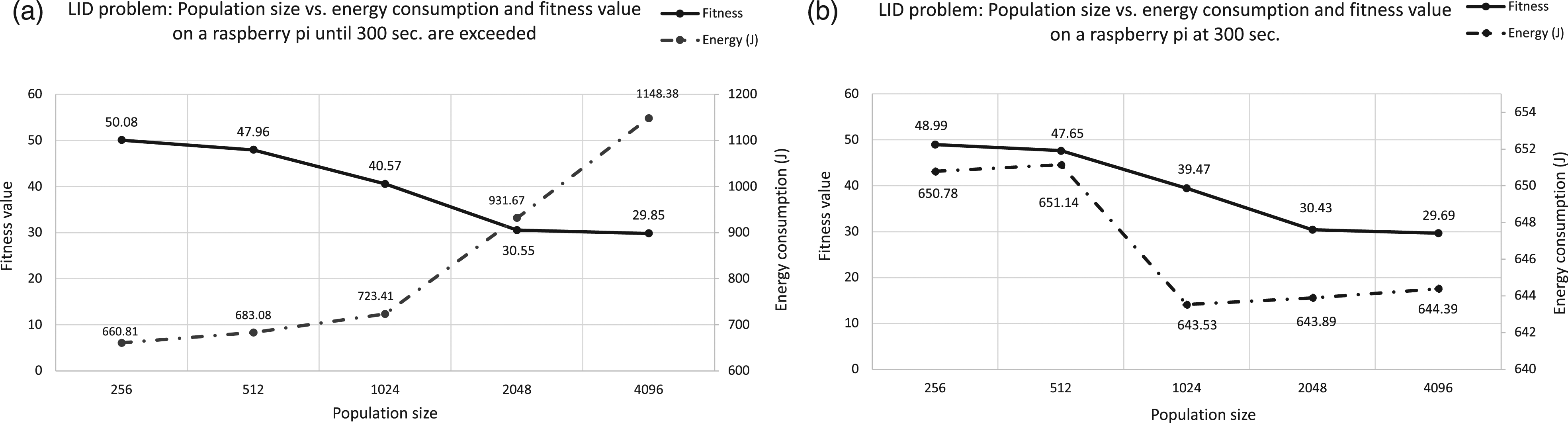

Regarding the fitness value, we can notice in both graphs included in the figure that in this experiment, with this time limit, the fitness value not only does not improve but also it gets worst when population size grows. This kind of behavior has already been shown in the literature, particularly in 2006 it was first described in Ref. 37: when a time limit is imposed a best population size exist to find the best possible solution in the allotted time.

We focus next on our main goal, the energy consumption. In order to do so, the energy consumption in graph (a) is analyzed and then an interesting behavior is observed: the larger the population size, the longer the runtime.

We must remember that the experiment can only finish when a generation is completed and the 300s time limit is surpassed. We can see in Figure 2 averaged fitness values and energy over 30 runs per population size: smaller population sizes produce short generations, and this influences shorter differences with the 300s time limit. Similarly, large populations require longer time per generation, and this means that the last generation after 300 s will be completed in a much longer time. Similarly, the larger the population size, the larger the energy required to complete the experiment, given that more time is required to complete the experiment.

Figure 2.

LID problem on Raspberry Pi. Analyzing the growth rates of execution time versus power consumption for each population size. X axis represents the population sizes and, Y axis is the growth rate values.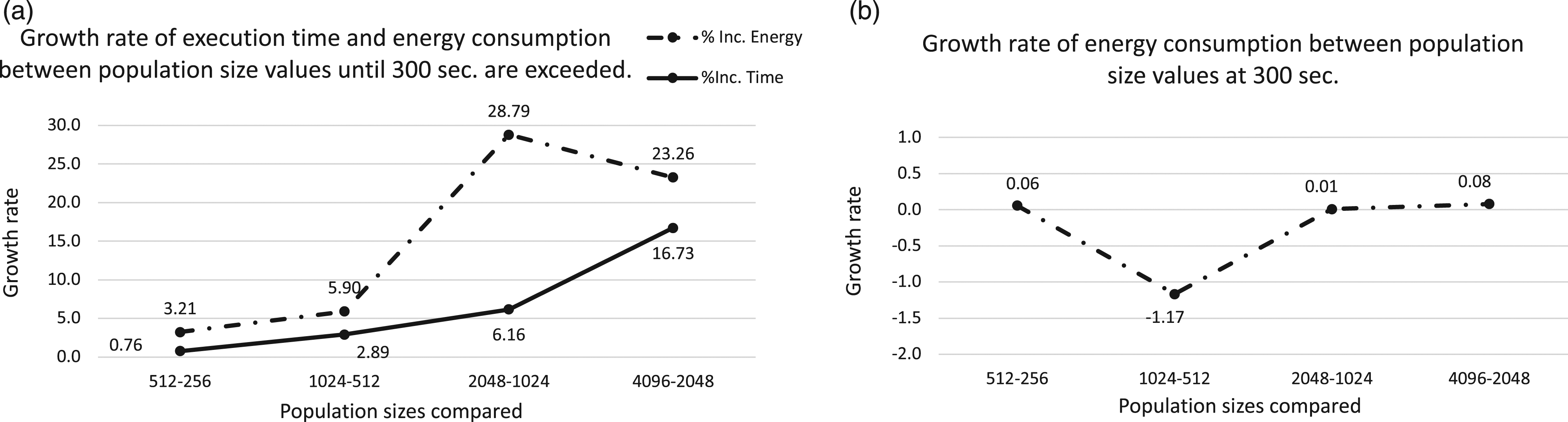

Yet, if we check Figure 2(a), we see that growth rate is not the same for running time as for power consumption. Moreover, some anomalies are found for some specific values (check the growth when comparing 1024 and 2048 for energy consumption).

It can be observed that the growth rate when small population sizes are used, is similar for both the energy consumption and execution time, although the growth rate of energy consumption is always a bit higher (i.e., population sizes = 256 and 512). However, it shoots up from size 1024 to 2048, being 26% higher than the time increase rate and, although between 2048 and 4096 the growth rate is more similar, this represents a 6% more.

On the other hand, Figure 2(b) represents the energy consumption at exactly 300 s. In this second experiment, we are measuring power consumption exactly at that time step, although it is not possible to catch fitness values at that point, given the way ECJ tool works, providing fitness values only after a generation is completed. Therefore, we include fitness values obtained in the last generation computed before 300 s are surpassed, so that we have an idea of the algorithm behavior.

We notice that differences found when comparing population sizes at 300 s are narrow, although some anomaly appears when comparing 1024 and 512 population sizes. Even though the difference is small, the energy consumption is a bit lower for 1024 individuals. Again, growth rates are shown in Figure 2(b), where the anomaly for 512 and 1024 population sizes is clearly shown.

This behavior could be seen at first sight as counter-intuitive given that the CPU is working at any time regardless of the operation performed. In the next sections, we try to confirm the anomalies detected, and then describe further experiments that tries to study why this is so.

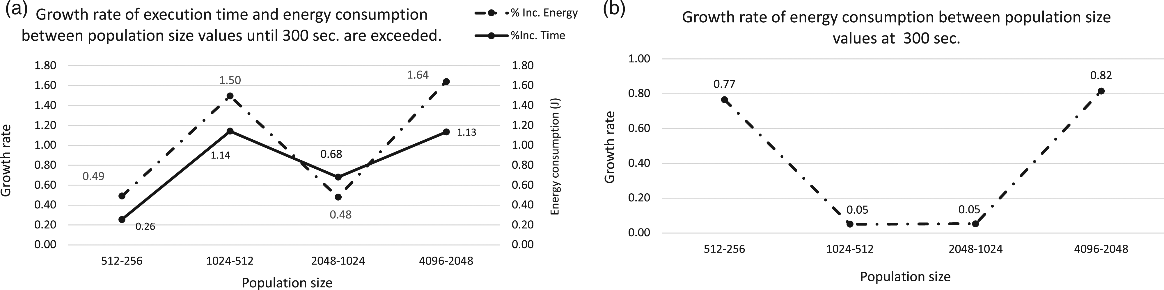
We address now the ORDER Tree problem. Figure 3 (Type #1) is described in the same terms as the previous one for the LID problem. As in the case of the fitness value for LID, the fitness value does not improve when population size grows: the smaller the size, the larger the fitness value. Similarly, if we analyze the energy consumption and we put the spotlight on Figure 3(a), we observe how energy consumption is increased as the size of the population grows. Despite the fact that this increase is not constant and the highest increases happen in the changes of population sizes from 512 to 1024 and from 2048 to 4096, differences are now smaller when compared to those obtained for LID. The evolution at 300 s Figure 3(b) is similar for both runtime and energy consumption. As it can be noticed in Figure 4 (Type 2), the growth rates are again narrow, but again differences are found even when all the measures are taken after exactly 300 s.

Figure 3.

ORDER Tree problem on Raspberry Pi. Analyzing the power consumption for different population sizes. X axis represents the population size, Y-left axis is the fitness value and Y-right axis corresponds to the power consumption. Graph (a) represents results including the excess time, and graph (b) results at the 300 s.

Figure 4.

ORDER Tree problem on Raspberry Pi. Analyzing the growth rates of execution time versus power consumption for each population size in a Raspberry Pi. X axis represents the population sizes and, Y axis is the growth rate values.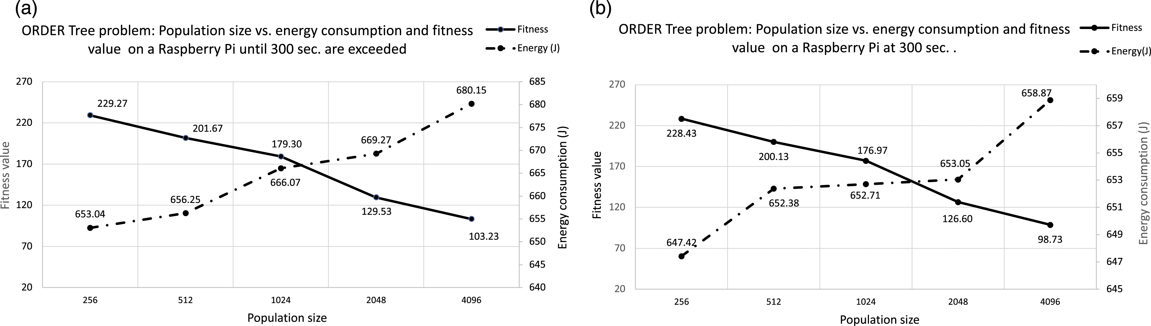

Results obtained in this specific experiment show significant variations in energy consumption across different population sizes, particularly for LID, and not so much for ORDER tree, at least in this hardware platform. This suggests that when addressing a real problem, power consumption should be a metric to be considered in the configuration of the algorithm’s parameters, although the problem itself induce differences in the energy required.

In any case, as the Raspberry Pi platform has limited hardware resources, more experiments on two additionally hardware platforms have been performed as described below, trying to confirm that the relationship between runtime and energy consumed is not linear, and that differences are influenced by parameter values selected for the algorithm.

x86 architecture

Once Raspberry Pi -ARM architecture—has been analyzed, we decided to repeat the experiments using the widespread x86 architecture. In this case, a Laptop and a PC have been considered. Moreover, given the availability of internal equipment to measure energy consumption, we have also employed this one together with the previous approach, as described in Methodology.

We begin this analysis using the laptop and still using the digital power meter Yokogawa WT310E for measuring the energy consumption.

With higher capacity in computing resources than a Raspberry Pi, we included the population size 8192 as a value to be analyzed in this experiment.

Figure 5 (Type #1) shows results obtained for LID. If we analyze both graphs (a) and (b), we observe a growing general trend similar to the one observed in previous experiments: the larger the population size, the higher the energy consumption. However, an exception appears with population size 256. Actually, the energy required to run a population size of 512 is 8.36% smaller than that of 256. We may notice that the total energy required for 256, is larger than the values for 512, 1024, and 2048. Therefore, although fitness value obtained using 256 individuals is slightly better, the larger energy consumption required, clearly shows for the first time, that specific values for population size are sometimes better when the goal is energy savings. This is quite an interesting behavior, given that it deviates from what we expected: the larger the population size, the higher energy consumption when we wait until a generation finished after more than 300 s. In any case, the most interesting result is shown in (b) graph: even when exactly 300 s have elapsed for each of the experiments, the 512 seems to be the population size tested that requires the smallest energy to reach that time step.

Figure 5.

LID problem on Laptop. Analyzing the power consumption for different population sizes on a laptop platform. X axis represents the population size, Y-left axis is the fitness value and Y-right axis corresponds to the power consumption. Graph (a) represents results including the excess time, and graph (b) results at the 300 s.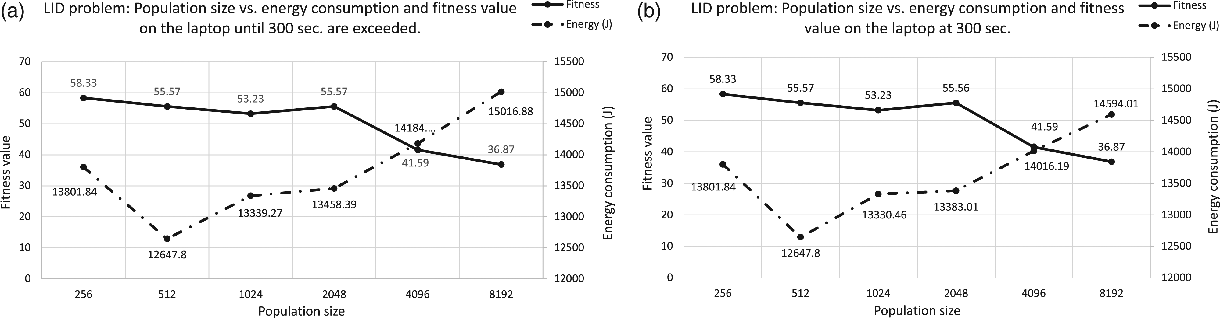

Figure 6 (Type #2) shows the respective growth rates between consecutive population sizes for LIDs on the laptop. We may notice that the highest growth rates appear when changing from 512 to 1024, 2048 to 4096, and 4096 to 8192, with 5.4%, 5.39%, and 5.87% percentages, respectively. These values are far from the growth rates for runtime 0.14%, 0.65%, and 1.23%, respectively. Although in most of the results shown when increasing runtime, the energy consumption also increases, the intensity with which it increases is not the same. There is not a perfect linear correlation. Could the reason behind this behavior be due to additional hardware or software resources, beyond the cpu, required for larger population sizes? As we will show below, this question requires further analysis.

Figure 6.

LID problem on Laptop. Analyzing the growth rates of execution time versus power consumption for each population size on a laptop platform. X axis represents the population sizes and, Y axis is the growth rate values.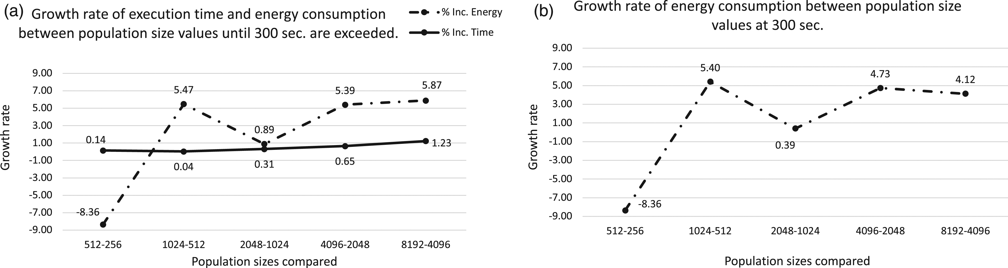

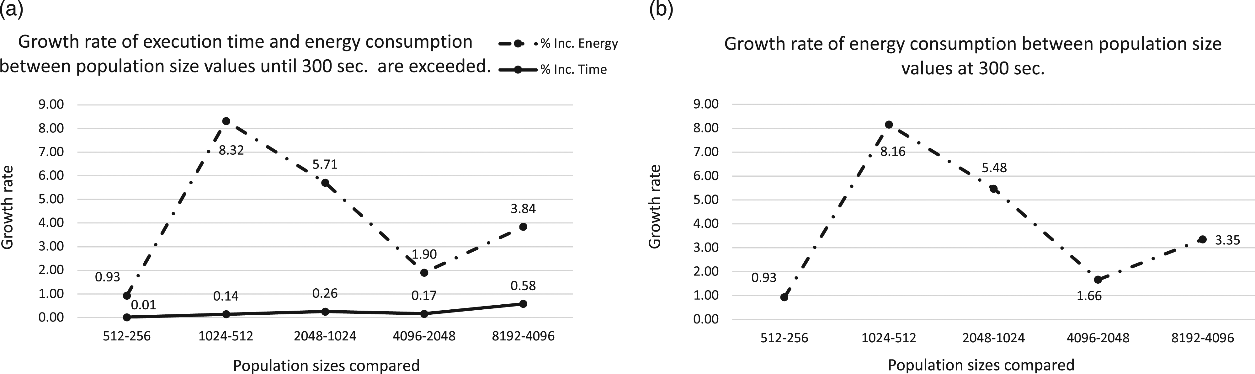
In similar terms, the results for ORDER, plotted in Figures 7 and 8, are analyzed and shown. The highest increase occurs from 1024 to 2048 with 8.32% and more sustained among the next consecutive population sizes. As it happens to LID, the time increase is lower than the energy consumption increasing with 0.58% as the highest percentage reached between 4096 and 8192, which confirm the trend shown before for the laptop.

Figure 7.

ORDER Tree problem on Laptop. Analyzing the power consumption for different population sizes on a laptop. X axis represents the population size, Y-left axis is the fitness value and Y-right axis corresponds to the power consumption. Graph (a) represents results including the excess time, and graph (b) results at the 300 s.

Figure 8.

ORDER Tree problem on Laptop. Analyzing the growth rates of execution time versus power consumption for each population size on a laptop. X axis represents the population sizes and, Y axis is the growth rate values.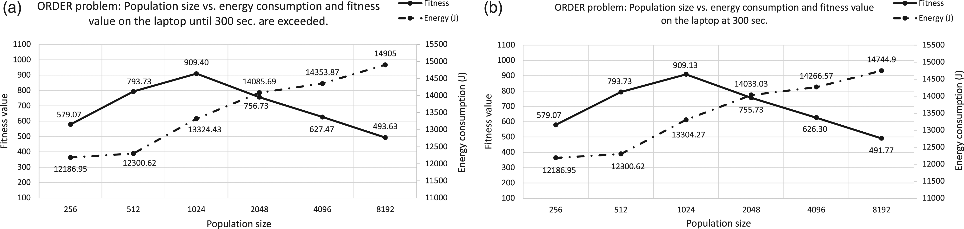

So, these differences need further research. Therefore, in the next section, we analyze a second x86 endowed device, and we apply energy measurement using a second method.

x86 & AppPowerMeter

In this case, a more powerful platform has been used to perform the experiments. As we previously mentioned, the measurements on this platform were taken through the AppPowerMeter software, which provides values for the energy consumed, the average power and the total time. Figure 9 shows the average values for both the energy consumption and fitness values. The graphs (a) correspond to results for LID and graph (b) for ORDER Tree.

Figure 9.

Analyzing the power consumption for different population sizes on PC platform. X axis represents the population size, Y-left axis is the fitness value and Y-right axis corresponds to the power consumption. Graph (a) represents results for LID problem and graph (b) results for ORDER Tree.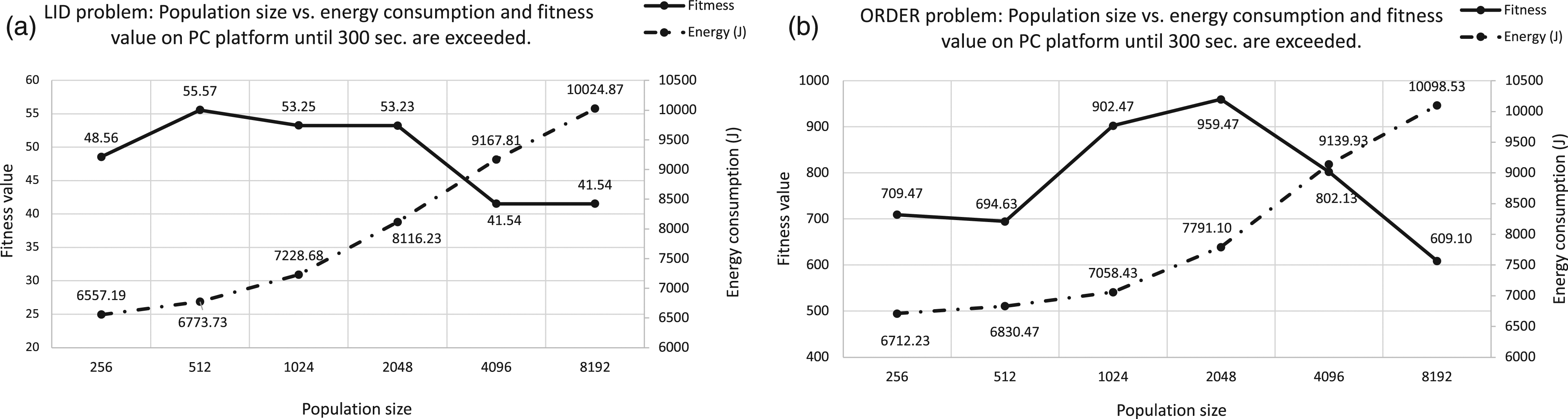

Regarding the fitness value, the trend is identical to the previous ones for Raspberry Pi and Laptop platforms. At the time established as limit, a degradation is produced on the fitness value. The behavior observed in relation to the energy consumption is also the same as that seen in the previous platforms and closer to the laptop for obvious reasons, in terms of the capacity of computing resources. On average, the amount of energy consumed on the laptop is higher than on the PC.

Figure 10.

Analyzing the growth rates of execution time versus power consumption for each population size on PC platform. X axis represents the population sizes and, Y axis is the growth rate values. Graph (a) corresponds to LID and (b) to ORDER Tree.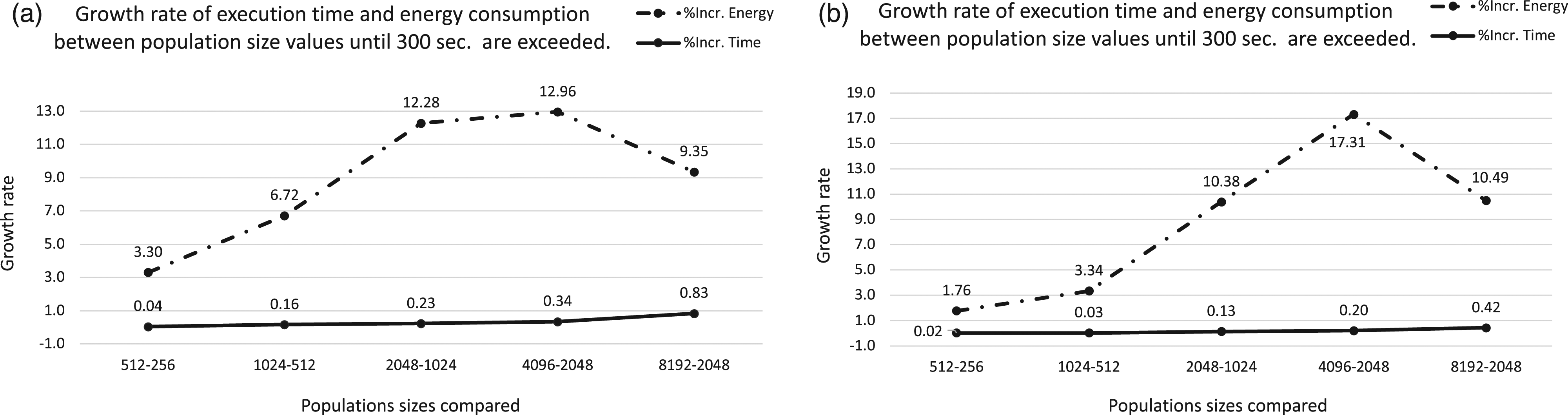

Figure 10(a) and (b) presents the growth rates of energy consumption and runtime, between consecutive population sizes for LID and ORDER Tree, respectively. The more relevant are differences when large population sizes are employed: For both benchmark problems, the time increase between consecutive population sizes never reaches 1%. However, the growth rate of energy consumption for larger population sizes exceeds 10% in all cases. In case of LID peaks at 12.28% and 12.96%, when changing from 1024 to 2048 and 2048 to 4096, respectively. With respect to ORDER Tree, a peak of 17.31% is registered when moving from 2048 to 4096. On the other hand, the energy increase we found when doubling population size from 4096 to 8192 is just around 10%. And comparatively, energy increase when doubling population size is never the double.

In any case, this confirms that the energy consumption is affected by parameters configuration, particularly in our case, by the population size.

The main conclusion is that energy consumed when running GP for 300 s varies influenced by population sizes, with some anomalies that show specific values as the best ones to reduce power consumption. Given that traditionally population sizes are chosen to optimize the fitness, this result shows that a new perspective should be considered: both measures should be taken into account when looking for an efficient way of finding solutions.

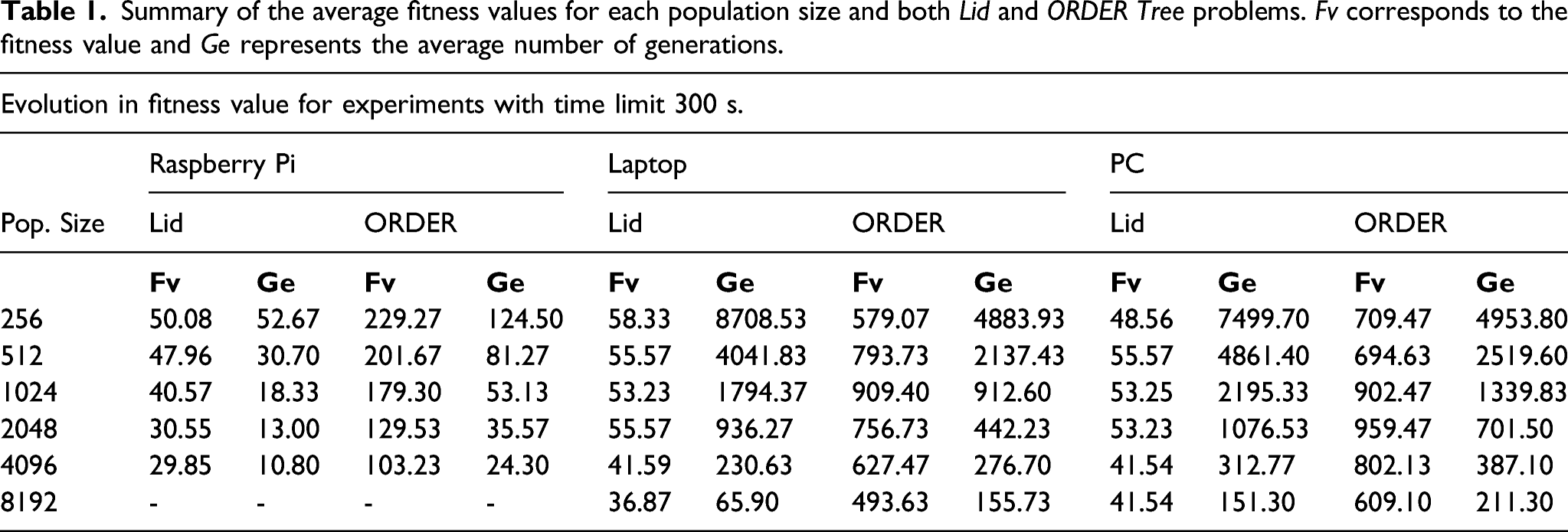
We are aware of differences found in each of the hardware platforms, that are due to different number of generations computed per experiment in each case, given hardware differences. Table 1 presents the evolution of fitness values and number of generations computed for each device. For each problem and population size, the average number of generations is also shown. As we see, large differences are found among platforms tested. Yet, all of them have shown a common trend regarding energy consumption: energy required depends on populations size employed.

Table 1.

Summary of the average fitness values for each population size and both Lid and ORDER Tree problems. Fv corresponds to the fitness value and Ge represents the average number of generations.

Evolution in fitness value for experiments with time limit 300 s.
	Raspberry Pi				Laptop				PC
Pop. Size	Lid		ORDER		Lid		ORDER		Lid		ORDER
	Fv	Ge	Fv	Ge	Fv	Ge	Fv	Ge	Fv	Ge	Fv	Ge
256	50.08	52.67	229.27	124.50	58.33	8708.53	579.07	4883.93	48.56	7499.70	709.47	4953.80
512	47.96	30.70	201.67	81.27	55.57	4041.83	793.73	2137.43	55.57	4861.40	694.63	2519.60
1024	40.57	18.33	179.30	53.13	53.23	1794.37	909.40	912.60	53.25	2195.33	902.47	1339.83
2048	30.55	13.00	129.53	35.57	55.57	936.27	756.73	442.23	53.23	1076.53	959.47	701.50
4096	29.85	10.80	103.23	24.30	41.59	230.63	627.47	276.70	41.54	312.77	802.13	387.10
8192	-	-	-	-	36.87	65.90	493.63	155.73	41.54	151.30	609.10	211.30

As we had previously seen, every hardware platform features some differences that affect power consumption: memory hierarchy, particularly cache sizes and levels, number of cores available, processor frequency, etc. Given that population size is related to memory consumption, processor frequency determines the time required to compute a generation, and so on and so for, clearly hardware platforms influence power consumption.

Running experiments until a fitness level is reached

The main goal when addressing an optimization problem through a standard EA is to find a solution good enough for the problem at hand. Thus, the EA can be run either for a given number of generations or can be configured to stop when a solution overpasses a specific fitness value. The question that arises in this second version stands as follows: How much energy would consume the algorithm to reach a solution with a specific quality level? How to find a balance between quality of solutions and energy consumed? Could we configure energy-efficient execution of the algorithm to not spend so much energy even if we have to obtain a bit worse solution?

Although it is not easy to find cut and clear answers to all those questions, in our next step, we designed an experiment on the PC platform for GP algorithm that hopes to provide some clues for further research in the future.

Again, we use ECJ with the same benchmark problems and population sizes. A conservative fitness quality to be reached was established: 60 and 960 for LID and ORDER Tree, respectively. Moreover, the value of the maximum number of generations to be executed if the given fitness value is not found was established at 1000.

As in previous experiments, 30 independent runs of the algorithm were performed and average values were computed. Figure 11 shows for each population size the fitness value obtained and the energy consumed till one of the stop conditions is met. This figure consists of two graphs, where graph (a) corresponds to LID problem and graph (b) to ORDER Tree. X axis represents the population size, Y-left axis denotes the fitness value and Y-right axis is the power consumption.

Figure 11.

Analyzing the power consumption for different population sizes on PC platform with a quality fitness value and a maximum number of generation as constraints. X axis represents the population size, Y-left axis is the fitness value and Y-right axis corresponds to the power consumption. Graph (a) represents results for LID problem and graph (b) results for ORDER Tree.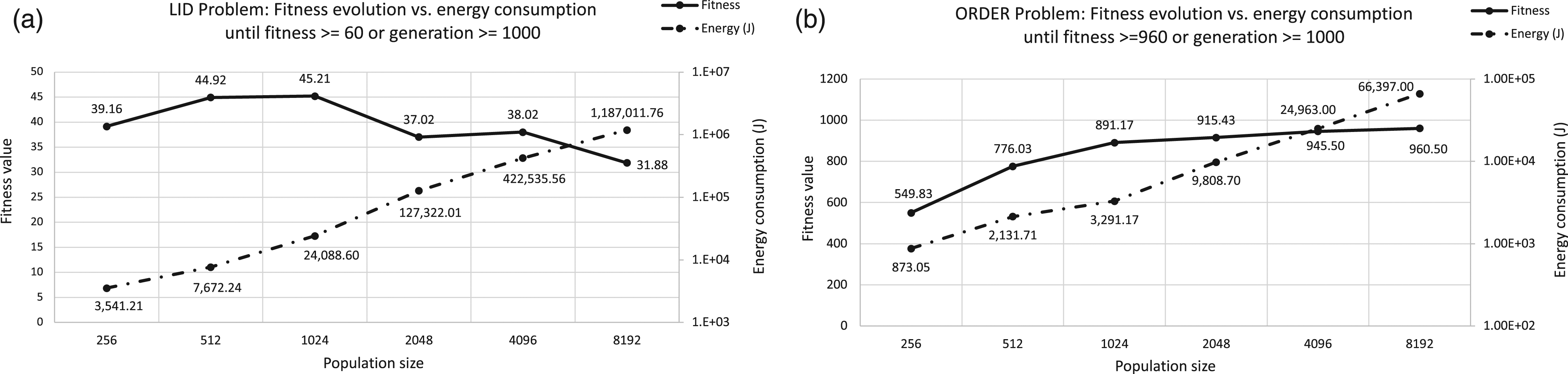

Regarding the fitness value, we may notice that for all population sizes in LID, the quality fitness level is not achieved while in ORDER Tree this is only reached with the largest population size (8192). Thus, all except one of the population sizes for ORDER Tree ended when 1000 generations were completed. We will now focus on the energy consumption and let’s first analyze the results obtained for the LID problem.

Table 2 presents the average values of the 30 runs for runtime, energy consumption, and fitness value for each population size and both problems.

Table 2.

Summary of the average values for each population size and LID and ORDER Tree problems.

LID
Pop. Size	Time	Energy consumption	Fitness
256	151.54	3541.21	39.16
512	302.89	7672.24	44.92
1024	782.86	24,088.60	45.21
2048	3598.70	127,322.01	37.02
4096	10,516.07	422,535.56	38.02
8192	29,514.00	1,187,011.76	31.88
ORDER Tree
Pop. Size	Time	Energy consumption	Fitness
256	36.90	873.05	549.83
512	88.73	2131.71	776.03
1024	132.04	3291.17	891.17
2048	342.32	9808.70	915.43
4096	735.31	24,963.00	945.50
8192	1760.16	66,397.00	960.50

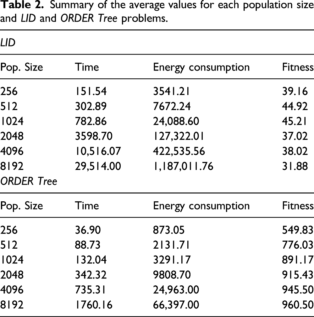
We may first compare the energy consumption between consecutive population sizes and we see that for each step from 256 to 8192, always increase over the previous energy value 2.16, 3.14, 5.24, 3.32, and 2.8 times, respectively. Nevertheless, when we examined the consecutive differences in the runtime—comparing each population size with the previous one, the total time is multiplied by 2, 2.58, 4.59, 2.94, and 2.8. The last one is the only one, where both values matched, time and energy consumption increase. So, we clearly see, that the relationship between time and energy is not linearly correlated.

We show in Figure 12 the results for ORDER Tree, where energy consumption increases for successive population sizes 2.44, 1.54, 2.98, 2.54, and 2.66, respectively. Similarly, for the runtime, we obtain 2.40, 1.49, 2.59, 2.14, and 2.39. As we can see, both values are closer for ORDER Tree than for LID.

Figure 12.

Analyzing runtime versus energy consumption for each population size on PC platform with a quality fitness value and a maximum number of generation as constraints. X axis represents the population size, Y-left axis is the energy consumption in Jules. Y-right axis corresponds to the time in seconds. Graph (a) represents results for LID problem and graph (b) results for ORDER Tree.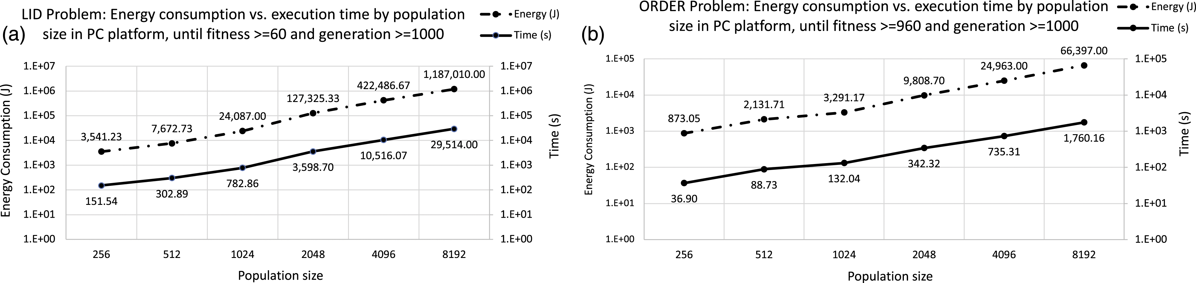

These results show us that every problem has a different behavior when considering energy consumption. The main conclusion is that we cannot assume that energy consumption does not deserve attention, as has been the case traditionally in the area. On the contrary, this topic should be more deeply analyzed for GP given the different behavior shown when analyzing computing time or quality of solutions. Moreover, in previous sections, we have shown that one of the most important GP parameter, population size, shows non-linear influences in energy required to find a solution as well as instantaneous energy consumption when a computer is running the algorithm.

All in all, we have not considered yet which could be the reason why different population sizes show different instantaneous energy consumption. In the next subsection, we try to shed light into this behavior.

Why does populations size influence instantaneous energy consumption?

In previous experiments, we had measured energy consumption of the whole computer, as a way to analyze algorithm energy behavior. But certainly, hardware resources, and also the operating system operations, may affect the energy values we measure. On the basis of this idea, and considering all the issues that may affect this behavior, we decided to carry out an additional test consisting of studying the cache memory. The idea behind this test is related to the specific parameter we are studying: population size. The reason is directly related to the nature of GP algorithm, that employs variable-size chromosomes.

Moreover, the bloat phenomenon³⁸ induces size growth as generations are computed, and this affects memory usage. Therefore, different values for population sizes will surely affect the use of memory, and particularly cache misses while the algorithm is running, which may induce changes in energy consumption. The cache memory system is one of the most energy-consuming components and it represents large share of processor power consumption.^39,40

In this experiment, we use the perf³ command^41,42 to access hardware performance counters, particularly counters for monitoring cache memory. Perf is a powerful open source performance monitoring tool, available in linux kernel, for tracking system events both hardware and software using a command line interface. It can also access the counters of the energy and power measurements provided through the Intel’s Running Average Power Limit (RAPL).

Therefore, we run the perf command customized with each benchmark problem and population sizes addressed. As a result, the statistic data collected for the cache memory were collected. This experiment analyzed cache misses, L1-Dcache load misses and L1-Dcache store misses. Cache misses are the number of non-served memory accesses by any of the caches, L1-Dcache load misses represents the number of non-served load accesses by the level 1 data cache, and L1-Dcache store misses is the number of non-served store accesses by the level 1 data cache.

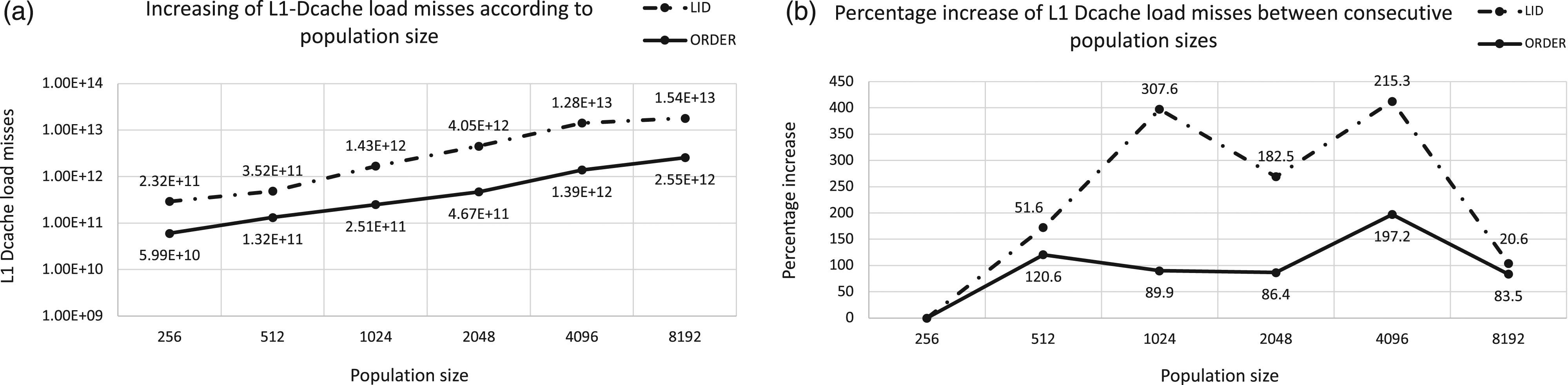
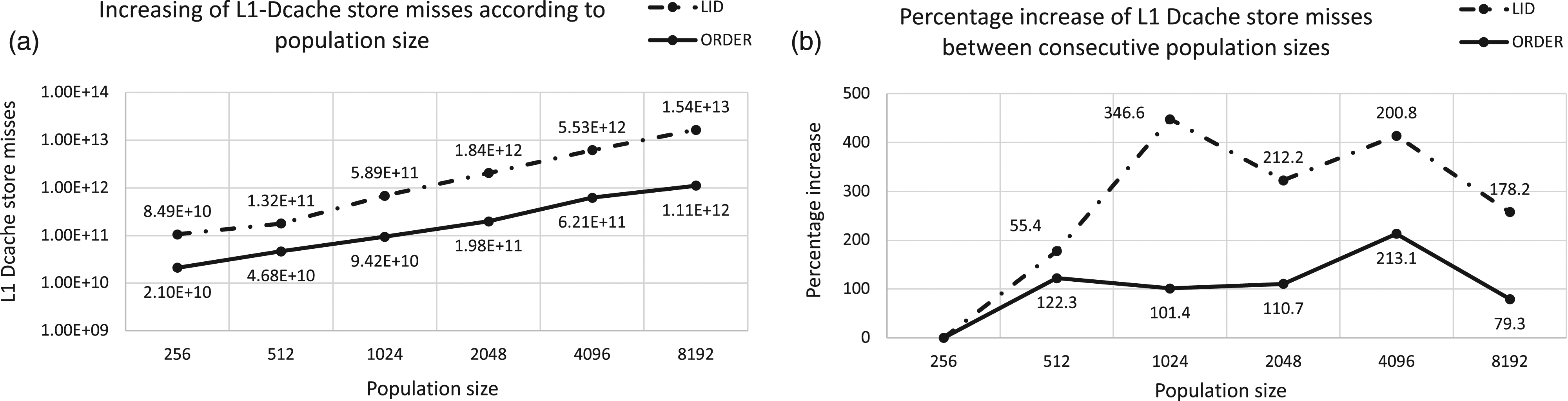
Figure 13 shows results for this monitoring experiment of the cache memory while our GP algorithm for LID and ORDER Tree is running. This figure consists of two graphs (a) and (b). The first one (a) plots the number of non-server memory accesses by the cache memory system, while the second one (b) plots the percentage increase between consecutive population sizes. It is interesting to see how there is an exponential growth in the number of cache misses as the population size grows, which leads the next level of the memory system to be accessed, the RAM memory or disk, in case the data is not found on RAM. This involves the activation of the access mechanisms to the corresponding hardware, which increases time and energy consumption. The memory cache monitoring for both benchmarks shows an exponential growth in the number of cache misses. In the case of LID from population size 1024, the percentage increase is always higher than 225% and the highest is reached between 512 and 1024 with 391.7% of misses. The number of cache misses in ORDER Tree grows also exponentially, and although with lower intensity it exceeds 100%, reaching the highest increase between 2048 and 4096 with 279.9%. Identical study was carried out on the L1 cache memory, particularly we measured the load misses and store misses to the data cache. Figures 14 and 15 show the L1-data-cache load and store misses, respectively. The design for both figures can be described in terms of Figure 13. Regarding the results obtained for load and store misses, these follow the same behavior than the number of non-served memory accesses by any of the caches.

Figure 13.

Analyzing the cache misses when running our GP algorithm on PC platform. Graph (a) represents the number of cache misses for each population size and Graph (b) plots the percentage increases of cache misses between consecutive population sizes. X axis represents the population size in both graphs and Y axis corresponds to the cache misses at logarithm scale in (a) and the percentage increases in (b). Dotted line on graphs corresponds to LID and the solid line represents ORDER Tree.

Figure 14.

Analyzing the L1-Dcache load misses when running our GP algorithm on PC platform. Graph (a) represents the number of L1-Dcache load misses for each population size and Graph (b) plots the percentage increases of misses between consecutive population sizes. X axis represents the population size in both graphs and Y axis corresponds to the cache misses at logarithm scale in (a) and the percentage increases in (b). Dotted line on graphs corresponds to LID and the solid line represents ORDER Tree.

Figure 15.

Analyzing the L1-Dcache store misses when running our GP algorithm on PC platform. Graph (a) represents the number of L1-Dcache store misses for each population size and Graph (b) plots the percentage increases of misses between consecutive population sizes. X axis represents the population size in both graphs and Y axis corresponds to the cache misses at logarithm scale in (a) and the percentage increases in (b). Dotted line on graphs corresponds to LID and the solid line represents ORDER Tree.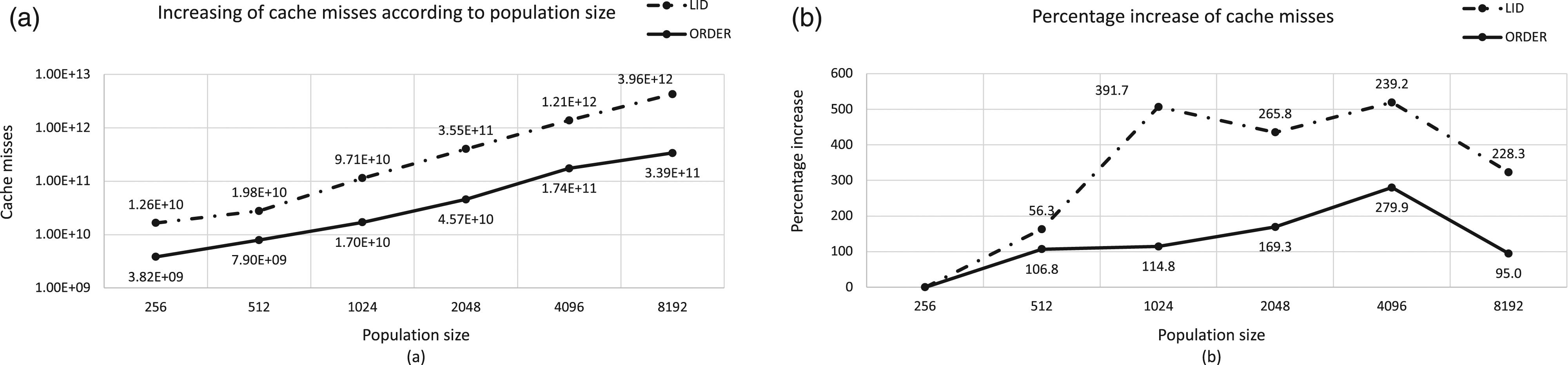

Based on the obtained results, we can confirm that the larger the population size, the higher the number of cache misses, which in some cases is one order of magnitude higher. This affects the energy consumed by the algorithm because it results in more frequent accesses to the main memory, which consume more energy than cache accesses.

In short and after this series of experiments, we can confirm that population size has an effect on EAs power consumption, particularly on GP, which is the objective of this work. We have identified that population size has an influence on energy consumption, at least partially due to cache memory usage. We have also seen that the increase of cache misses is not proportionally correlated to population size increase. Moreover, we have seen that energy consumption is not directly correlated with runtime of the algorithm.

We can thus conclude that although processors maybe working similarly regardless of the population size values employed when running GP, other factors affect energy consumption, and therefore the relationship between quality of solution found and energy required to find that solutions.

Although more experiments will be required for a better understanding of this phenomenon, a clear conclusion is reached here: the main parameters of the algorithm influences energy consumption, and this topic deserves attention in the future if we want to reach energy-efficient GP and also EAs.

Conclusions

This paper addresses a topic that has been scarcely considered before in the area of Evolutionary Algorithms: the possible influence that parameter values may have on energy required to reach a solution.

We have thus selected population size as the main goal for the analysis presented, and have compared how much energy is required to run the algorithm in three different scenarios: (a) Until 300 s are surpassed after computing a generation; (b) Exactly after running the algorithm 300 seconds; (c) when a given fitness quality is looked for or a maximum number of generations computed.

The results have shown something of interest. On the one hand, the energy consumption is not directly correlated with runtime. Secondly, population size influences energy consumed, but again, there is not a direct relationship between size and energy required to complete the experiment. Moreover, in some experiments, for certain population size values, smaller generations require more energy than larger ones. This means that population size not only influences quality of results, but also energy consumed, and therefore a deeper study is required to understand the relationship between quality of solutions, parameter values, and energy required to reach such solutions.

Finally, we have also tried to see why the above-described results have been found, considering population size and energy. We have thus studied possible influence of cache memory—given that GP is particularly affected by memory problems due to variable-size chromosomes—and have seen that the number of cache misses is not proportional to population size, and therefore further studies will be useful in the future to perfectly understand and choose appropriate values for GP and EA parameters.

All in all, this paper paves the way to future research on the influence and proper selection of GP and EA main parameters when looking for energy-efficient algorithms.

Footnotes

Acknowledgements

We acknowledge support from Spanish Ministry of Economy and Competitiveness under project TIN2017-85727-C4-\{2,4\}-P. Grant PID2020-115570GB-C22 and PID2020-115570GB-C21 funded by MCIN/AEI/10.13039/501100011033. Junta de Extremadura under project GR15068.

Declaration of conflicting interests

The author(s) declared no potential conflicts of interest with respect to the research, authorship, and/or publication of this article.

Funding

The author(s) disclosed receipt of the following financial support for the research, authorship, and/or publication of this article: This work was supported by the Spanish Ministry of Economy and Competitiveness under project TIN2017-85727-C4-\{2,4\}-P. Grant PID2020-115570GB-C22 and PID2020-115570GB-C21 funded by MCIN/AEI/10.13039/501100011033. Junta de Extremadura under project GR15068.

ORCID iD

Josefa Díaz-Álvarez

Notes

References

Gelenbe

Caseau

. The impact of information technology on energy consumption and carbon emissions.Ubiquity 2015; 2015: 1–15. DOI: 10.1145/2755977.

Fettes

Clark

Bunescu

, et al. Dynamic voltage and frequency scaling in NoCs with supervised and reinforcement learning techniques. IEEE Trans Comput 2019; 68(3): 375–389. DOI: 10.1109/TC.2018.2875476.

Arroba

Moya

Ayala

, et al. Dynamic voltage and frequency scaling-aware dynamic consolidation of virtual machines for energy efficient cloud data centers. Concurrency Comput Pract Exper 2017; 19(10): e4067. DOI: 10.1002/cpe.4067.

Haj-Yahya

Alser

Kim

, et al. Sysscal exploiting multi-domain dynamic voltage and frequency scaling for energy efficient mobile processors. In: 2020 ACM/IEEE 47th Annual International Symposium on Computer Architecture, 30 May-3 Jun, Valencia, Spain: ISCA, 2020, pp. 227–240. DOI: 10.1109/ISCA45697.2020.00029.

Xie

Zeng

Xiao

, et al. Energy-efficient scheduling algorithms for real-time parallel applications on heterogeneous distributed embedded systems. IEEE Trans Parallel Distributed Syst 2017; 28(12): 3426–3442. DOI: 10.1109/TPDS.2017.2730876.

Wang

. Feedback cache mechanism for dynamically reconfigurable VLIW processors. Tsinghua Sci Technol 2017; 22(3): 303–316. DOI: 10.23919/TST.2017.7914202.

anohar

Kapoor

. Dynamic reconfiguration of embedded-DRAM caches employing zero data detection based refresh optimisation. J Syst Archit 2019; 100: 101648. DOI: 10.1016/j.sysarc.2019.101648.

Mota

Azam

Shanmugam

, et al. Comparative analysis of different techniques of encryption for secured data transmission. In: 2017 IEEE international conference on power, control, signals and instrumentation engineering. ICPCSI), Chennai, India, 21-22 September 2017, pp. 231–237. DOI: 10.1109/ICPCSI.2017.8392158.

Kong

Pan

Snášel

, et al. An energy-aware routing protocol for wireless sensor network based on genetic algorithm. Telecommun Syst 2018; 67: 451–463, DOI: 10.1007/s11235-017-0348-6 .

. Energy consumption analysis of algorithms implementations. In: 2015 ACM/IEEE International Symposium on Empirical Software Engineering and Measurement. Beijing: ESEM, 22-23, October 2015, pp. 1–4. DOI: 10.1109/ESEM.2015.7321198.

. Energy consumption analysis of image encoding and decoding algorithms. In: IEEE/ACM 4th International Workshop on Green and Sustainable Software, Florence, 18 May, 2015, IEEE, pp. 15–21. DOI: 10.1109/GREENS.2015.10.

, et al. From ephemeral computing to deep bioinspired algorithms: new trends and applications. Future Gener Comput Syst 2018; 88: 735–746. DOI: 10.1016/j.future.2018.07.056 .

13.

El-Ghazali

. A unified view of parallel multi-objective evolutionary algorithms. J Parallel Distributed Comput 2019; 133: 349–358. DOI: 10.1016/j.jpdc.2018.04.012 .

14.

Dargie

. A stochastic model for estimating the power consumption of a processor. IEEE Trans Comput 2015; 64(5): 1311–1322. DOI: 10.1109/TC.2014.2315629.

, et al. Looking for energy efficient genetic algorithms in artificial evolution. In: Idoumghar

Legrand

Liefooghe

(eds) Artificial Evolution EA 2019. Lecture Notes in Computer Science. Cham: Springer, 2019, Vol. 12052, pp. 96–109. DOI: 10.1007/978-3-030-45715-0_8 .

16.

Albers

. Energy-efficient algorithms. Commun ACM 2010; 53: 86–96, DOI: 10.1145/1735223.1735245 .

, et al. A review of energy-efficient scheduling in intelligent production systems. Complex & Intelligent Systems 2020; 2: 237–249. DOI: 10.1007/s40747-019-00122-6.

, et al. A genetic algorithm for minimizing energy consumption in warehouses. Energy 2016; 114: 973–980. DOI: 10.1016/j.energy.2016.08.045 .

, et al. An evolutionary scheduling approach for trading-off accuracy vs. verifiable energy in multicore processors” in Logic J the IGPL 2017; 25(6): 1006–1019, DOI: 10.1093/jigpal/jzx048 .

. An integer linear programming model and adaptive genetic algorithm approach to minimize energy consumption of cloud computing data centers. Comput Electr Eng 2018; 67: 551–565. DOI: 10.1016/j.compeleceng.2018.02.028\enleadertwodots .

, et al. Energy-efficient algorithms. In: Proceedings of the 2016 ACM Conference on Innovations in Theoretical Computer Science, Cambridge Masachusetts USA, 14-17 January 2016, pp. 321–332.

, et al. Estimation of energy consumption in machine learning. J Parallel Distributed Comput 2019; 134: 75–88. DOI: 10.1016/j.jpdc.2019.07.007 .

. A component-based study of energy consumption for sequential and parallel genetic algorithms. J Supercomput 2019; 75: 6194–6219. DOI: 10.1007/s11227-019-02843-4 .

24.

O’Neill

Lee

. Automatic programming: The open issue? Genetic Programming and Evolvable Machines, 2019; 21: 1–12.

, et al. Genetic programming needs better benchmarks. In: Proceedings of the 14th annual conference on Genetic and evolutionary computation (GECCO ’12), Philadelphia Pennsylvania USA, 7-11 July 2012. New York, NY, USA: Association for Computing Machinery, pp. 791–798. DOI: 10.1145/2330163.2330273 .

, et al. A cross-platform assessment of energy consumption in evolutionary algorithms. In: Parallel problem solving from nature – PPSN XIV Lecture Notes in Computer Science. Cham: PPSNSpringer, 2016, pp. 548–557. DOI: 10.1007/978-3-319-45823-6_51 .

, et al. A fuzzy rule-based system to predict energy consumption of genetic programming algorithms. Computer Sci Inf Syst 2018; 15: 635–654. DOI: 10.2298/CSIS180110026A.

28.

Freeborn

. Performance evaluation of raspberry Pi platform for bioimpedance analysis using least squares optimization. Pers Ubiquit Comput 2019; 23: 279–285, DOI: 10.1007/s00779-019-01203-6 .

29.

Zhuang

, et al. Parameter estimation of lorenz chaotic system based on a hybrid jaya-powell algorithm. IEEE Access 2020; 8: 20514–20522. DOI: 10.1109/ACCESS.2020.2968106.

30.

Yokogawa Electronic Corporation . Digital PowerMeter WT310E. 2020. https://www.yokogawa.com (accessed 24 August 2020).

31.

Spencer

Paradis

Vincent

, et al. A validation of DRAM RAPL power measurements. In: Proceedings of the Second International Symposium on Memory Systems (MEMSYS ’16). New York, NY, USA: Association for Computing Machinery; 2016, pp. 455–470. DOI: 10.1145/2989081.2989088.

32.

Intel . Intel 64 and IA-32 architectures software developer’s manual. Volume 3B, 2017. https://software.intel.com/en-us/articles/intel-sdm (accessed 24 August 2020).

33.

Khan

Hirki

Niemi

, et al. RAPL in action: experiences in using RAPL for power measurements. ACM Trans Model Perform Eval Comput Syst 2018; 3(2): 1–26, DOI: 10.1145/3177754.

34.

Garcia

. Exploration of energy consumption using the intel running average power limit interface. In: IEEE Space Computing Conference (SCC), Pasadena, CA, USA, 30 July-1 August 2019, IEEE Space Computing Conference (SCC), 2019, pp. 1–10. DOI: 10.1109/SpaceComp.2019.00005.

35.

Luke

, ECJ then and now. In: Proceedings of the Genetic and Evolutionary Computation Conference Companion (GECCO ’17), Berlin, 15-19 July 2017, New York, NY, USA: Association for Computing Machinery, pp. 1223–1230. DOI: 10.1145/3067695.3082467 .

36.

Scott

Luke

. ECJ at 20: toward a general metaheuristics toolkit. In: Proceedings of the Genetic and Evolutionary Computation Conference Companion (GECCO ’19), Prague, 13-17 July New York, NY, USA: Association for Computing Machinery; 2019, p. 1391. DOI: 10.1145/3319619.3326865 .

37.

Piszcz