Sage Journals: Discover world-class research

Abstract

The design and implementation of a performance protocol for local seismicity monitoring, is presented. A low-cost seismograph was installed in an area of high seismic activity in Evgiros, Lefkada Island, Greece, collocated with a high resolution 24-bit digitizer equipped with a broadband seismometer. A testing list of 28 local events with different epicenters and magnitudes has been compiled while acquisition data from the conventional seismograph and the proposed one were analyzed. Stochastic data analysis was used to compare these recordings on the same test site with different logging devices. The obtained results showed a satisfactory outcome in the performance of the proposed low-cost seismograph. Even though noise was present, P and S waves were clearly recorded with distinct amplitudes and therefore this arrival time difference, when compared with the one originating from the conventional seismograph, was found to be insignificant. Moreover, through a known magnitude equation, it manages to calculate earthquake’s local magnitude with a deviation of ± 0.4, a result that can be further improved. Lastly, spectral content analysis revealed almost identical waveforms with equivalent relative frequency distributions between the devices being compared.

Keywords

seismicity tectonics data analysis signal processing low-cost instrumentation dense monitoring network

Introduction

In order to monitor seismicity with high accuracy as well as to understand in detail the crustal processes,^1,2 seismological networks with a few kilometers interstation distance are required.^3–6 The need to upgrade and enrich any available seismic instrumentation is an ongoing process and many approaches have been introduced in recent years.^7,8 Due to the high cost of the deployed instrumentation, this aforementioned interstation distance has only been possible, up to now, for specific research projects^9,10 that involved dense instrumentation using portable equipment for a short period of time.^11,12 Even in countries with dense seismic networks, the station density is not highly adequate.^13–15 Current developments on sensor technologies and analog-to-digital converters (ADC) enable the design of low cost, low noise and high resolution seismographs.^4,16,17 Many research groups have tried in the recent years to develop their own equipment. For example, Llorens et al.¹⁶ developed Geophonino, an Arduino-based recording system with a vertical geophone, suitable for seismic surveys. Two years later, Llorens et al.¹⁸ presented Geophonino 3D, a three-component low-cost seismic recorder, suitable for passive seismic measurements. Also, Bravo et al.¹⁹ proposed a low-cost sensing system for recording accelerations with a MEMS (Micro Electro-Mechanical Systems) analog acceleration sensor, using a linear shake table to reproduce strong-motion recordings from actual earthquakes. All these sensing techniques include the Arduino Uno microcontroller. Moreover, Karakostas and Papanikolaou 4 presented a low-cost accelerograph, based on Atmel ATmega328P microcontroller and an acceleration sensor, with main objective to capture a detailed view of strong motion distribution in urban areas during seismic events. In addition, Holmgren and Werner²⁰ evaluated the performance of a low-cost network of private Raspberry Shake (RS) seismographs and vertical geophones, aiming to record ground motions of induced microseismicity. The low-cost Raspberry Shake (RS) seismometer was also used by Calais et al.²¹ to monitor Haiti’s earthquakes.

Nowadays, the cost for a high resolution (24 bit) digitizer equipped by a broadband seismometer is about 15.000 euros. Our aim is to propose cost-effective recording systems with development cost of about 400 to 1.000 euros, much lower than the cost of a conventional seismograph. The low construction cost allows the development and installation of a dense monitoring network, as well as the maintenance and regular operation of this network for many years, since it is common to use seismographs only for the special needs of a project and after its completion the maintenance is economically unprofitable. Under this framework, a properly large network of seismological stations could be used on a permanent basis. In this way, the signal analysis of this very dense seismological network will reveal the effects of the multiscale nature of active faults as well as those of seismic wave interactions with terrestrial inhomogeneous materials along its path to the crust.³ After the successful completion of the hardware implementation,²² the current research focuses on proposed seismograph’s pilot testing under real conditions, with the aim of reliably recording low magnitude earthquakes within a radius from 4 km to 18.5 km. The basic hardware elements of the proposed seismograph are firstly described along with sensors specifications and system’s general capabilities and information on the research area and the method used is followed. Then, a seismic catalog consisting of 28 typical and representative events has been created and then signal processing analysis was performed, as Figure 1 highlights. The approach used included first arrival time picking, magnitude calculation as well as frequency content investigation through spectral analysis between the proposed low-cost seismograph and the conventional one. Finally, all the results were compared in order to examine the performance efficiency of the proposed low-cost seismograph.

Figure 1.

Flowchart of the method followed, showing the initial steps from event selection and retrieval of raw data to signal processing, analysis and comparison of results.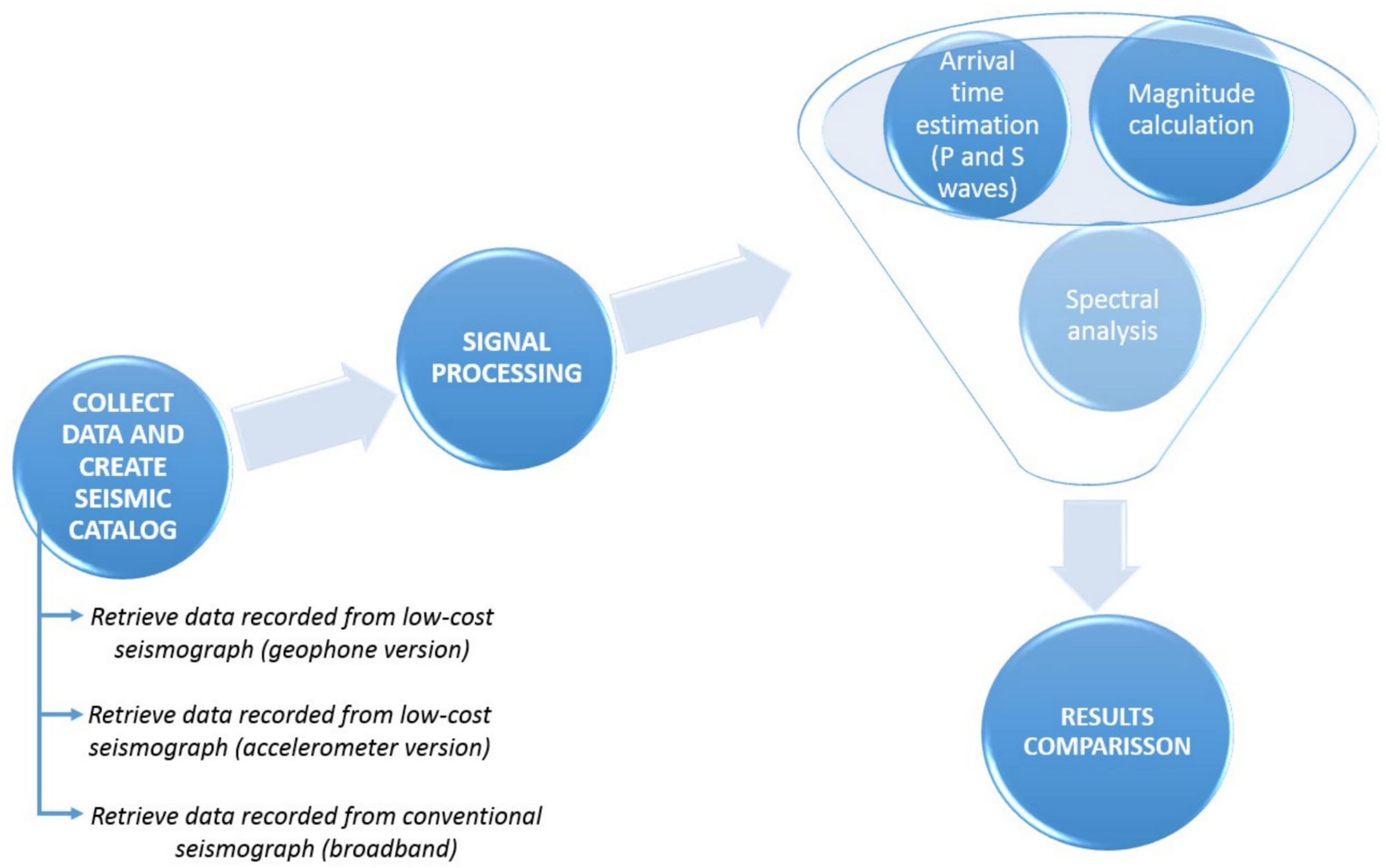

Hardware specification for local seismicity monitoring

Intending to measure ground vibrations and monitor local seismicity as well as the evolution of an earthquake sequence through a dense seismic network, a new cost-effective sensing unit was proposed.²² The general structure of the system developed for single-component (vertical) seismic data acquisition is illustrated in Figure 2. It is based on a Raspberry Pi 3B+ microprocessor board and an Arduino Uno R3 single microcontroller board, focusing this way on low construction cost. The Raspberry Pi 3B+ is the fundamental device while the Arduino Uno R3 operates as a 10bit analog to digital converter (ADC). The reason on using an Arduino Uno instead of adding an analog to digital converter was mainly to keep the design cost of the proposed system in very low levels. Each system encompasses one sensor with the ability to easily adapt new ones. Figure 2 depicts the single-axis (vertical) ceramic accelerometer (KB12VD), the single-axis (vertical) moving coil geophone (GS11D) as well as the operating frequency range according to the sensors specification limitations.^23,24. The operating frequency range equals from lower (-3db) to upper (-3db) limit: 0.5 Hz–45 Hz for the accelerometer and 4.5 Hz–45 Hz for the geophone.

Figure 2.

Proposed advanced, cost-effective and low-power seismic station ready for installation, along with the conventional sensors used during the development phase (upper part). The Geospace GS-11D Vertical geophone with its characteristics (lower part-left) and the Innomic IEPE KB12(VD) piezoelectric accelerometer with its characteristics (lower part-right).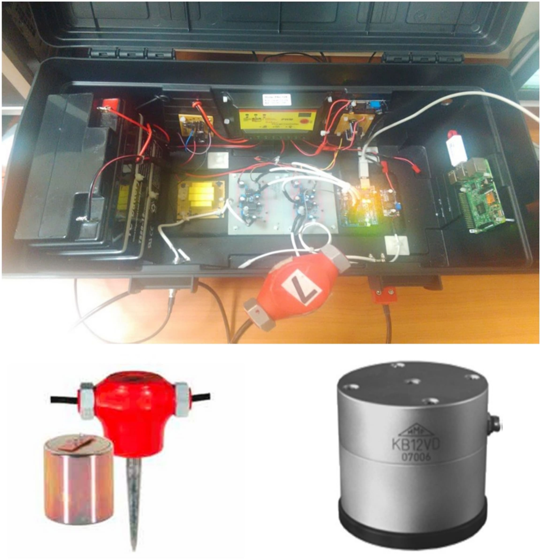

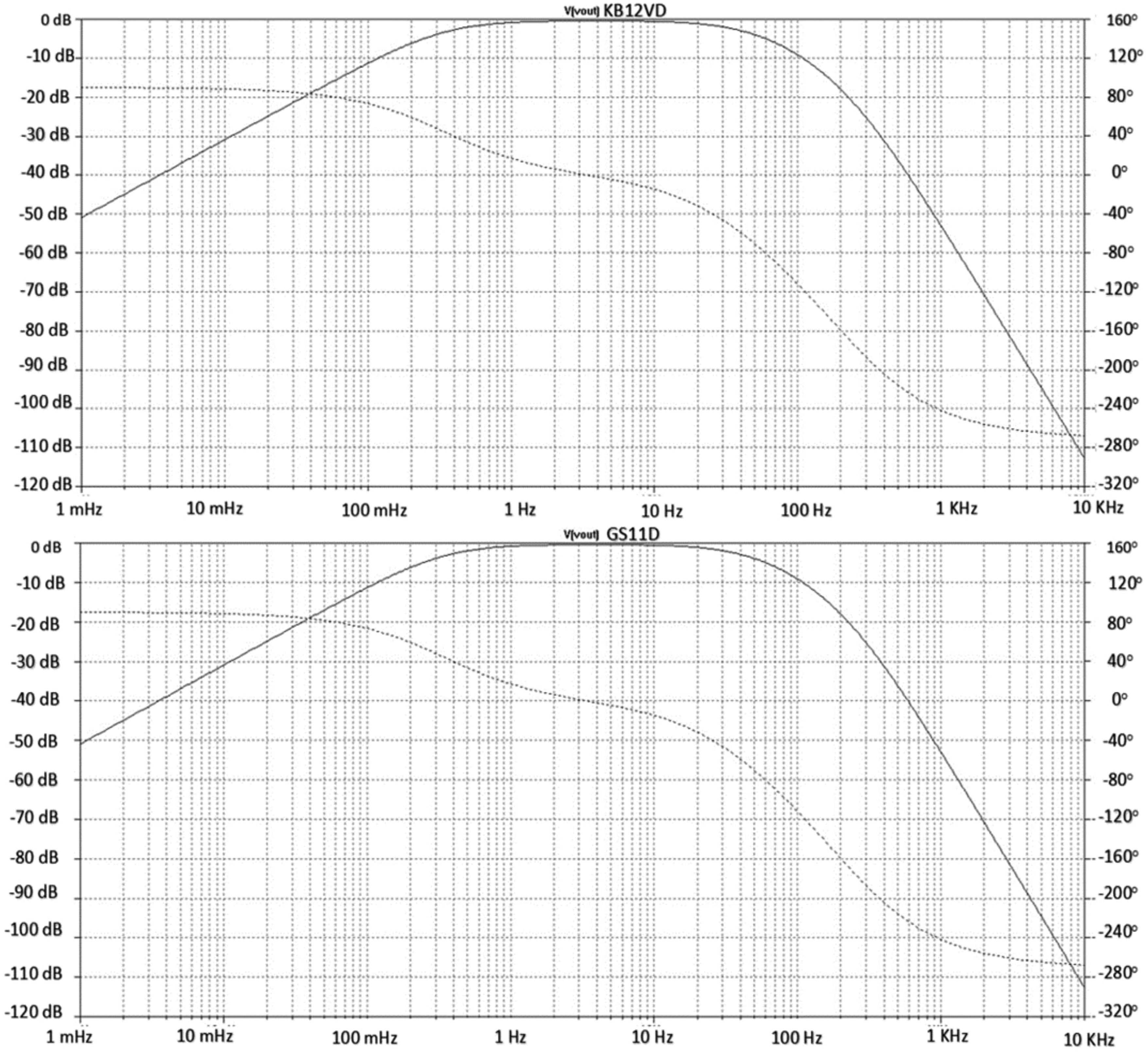
To increase the sensitivity of the two sensors, high gain amplification had to be achieved, neither changing their initial frequency and phase specifications nor importing any kind of external noise on it. For this reason, two high gain-low noise signal preamplifiers were designed, one for each version, as illustrated in Figure 3. Sophisticated simulation tools and PCB (printed circuit board) development software tools were used, as the sensor had to perfectly fit with the preamplifier at the lowest noise level. To be more specific, the LTSPICE open-source simulation software was used, to develop and improve the electronic design of the preamplifier as well as to improve the antialiasing filter. The two sensors signals are independently amplified by a factor (A) which is the signal output divided by the signal input without any distortion. The preamplifier for each version consists of two operational amplifiers and two stages of amplification. Assuming V3 is the sensors signal output, the U1 operational amplifier amplifies this signal by a factor X. Then, the signal passes from a high pass filter to eliminate DC interference and after that the U2 operational amplifier amplifies it again by a factor X1. The amplified signal finally passes from a first order passive low pass filter that eliminates the output frequency response at -3db to 45 Hz and comes to the output (V_out) of the amplifier, as shown in Figure 4. The amplification total factor equals to X × X1 and differs for each preamplifier due to the different characteristics of each sensor. For each sensor (KB12VD accelerometer and GS11D geophone), a unique PCB board was designed. The Express PCB software was then used to design the printed circuit board of the sensor signal amplifier. After component implementation, laboratory testing through breadboard simulation tests and calibration, both designed signal amplifiers were incorporated to each low-cost acquisition device.

Figure 3.

Schematic representation of signal preamplifiers for accelerometer KB-12VD (up) and geophone GS-11D (down).

Figure 4.

Bode diagrams (Amplification vs Frequency) of the preamplifier for the accelerometer KB12VD (up) and for the geophone GS11D (down). Upper Corner frequency -3db = 45 Hz.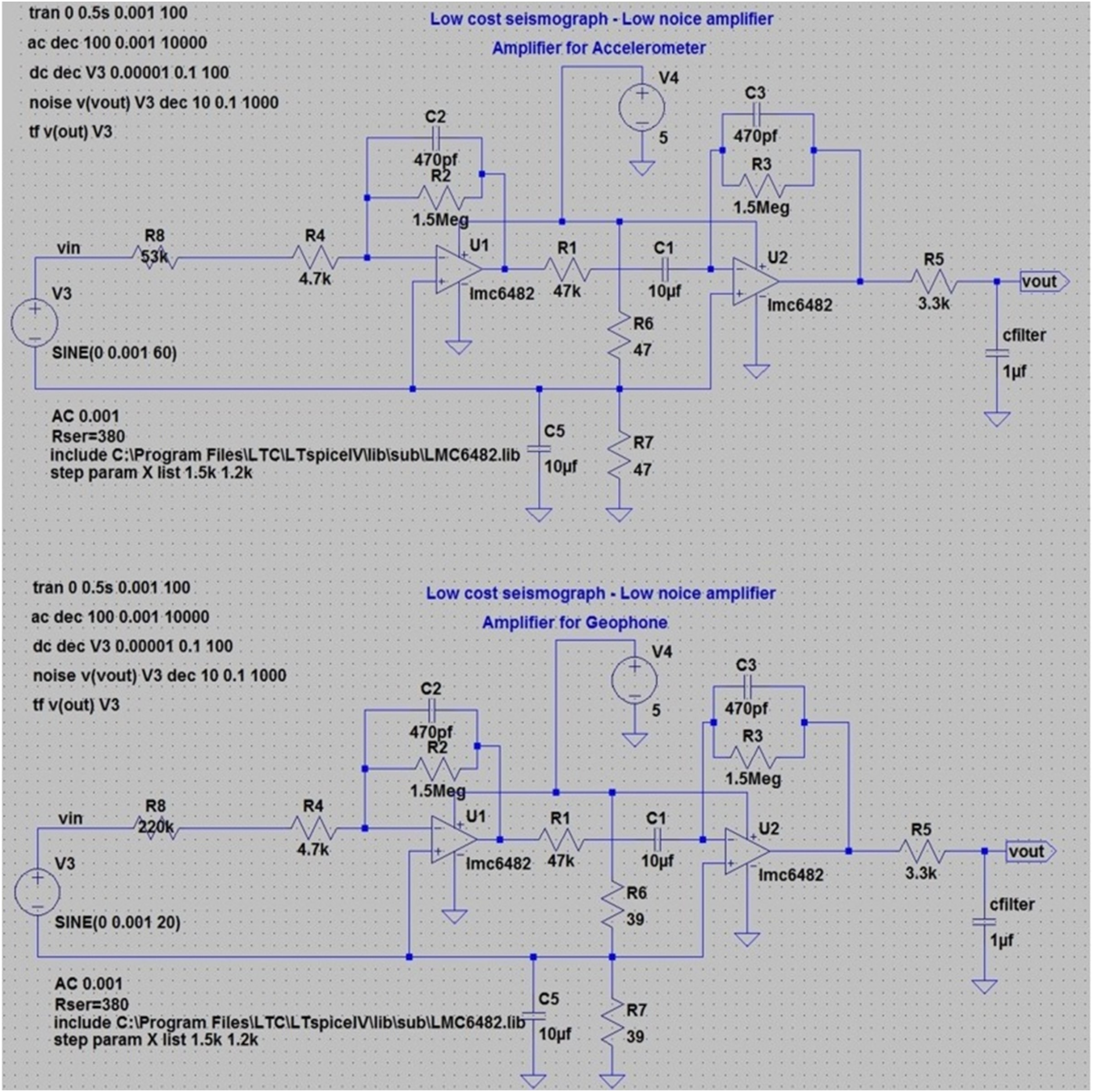

Further analyzing the operation principle of the low-cost systems, the microcontroller board (Arduino Uno R3) is responsible for digitizing the amplified signal (analog data) from the two sensors with a sampling frequency ranging up to 1 kHz. The sampling frequency was currently set to 345 Hz, oversampling more than three times the signals, compared with broadband sampling frequency (100 Hz). Thus, the digitized data are imported to the low-cost microprocessor board (Raspberry Pi3B+). Keeping in mind that the proposed low-cost seismograph has access to the Internet, in normal operation, the system is adding timestamp through an external highly accurate Real Time Clock board (DS3231 model), which is connected directly to the microprocessors input pins and is in continuous synchronization with the NTP (Network Time Protocol) server time. On the other hand, the conventional seismograph uses satellite GPS synchronization. Thus, the only limitation we have is to secure that a continuous connectivity to the internet is established. In case of Internet connectivity loss and during this time period a new earthquake occurs, the proposed low-cost seismograph will record this event and the recorded data will continue to have timestamp from the real time clock (RTC - model DS3231) with an NTP error of 3.52 s for 24 h without Internet, which is an extremely rare case as the connectivity loss duration usually ranges from a few minutes to a few hours. The above-mentioned maximum synchronization deviation without Internet (3.52 s in 24 h) equals to 4.07 e^-5 s in every second, until the connectivity is restored and this error resets. So, the maximum period without synchronization is defined as the time period that there is no connectivity to the Internet. Nevertheless, the absolute timing differences between the two systems are insignificant, because when the connectivity is restored, the real time clock synchronizes again with the NTP server and the error resets.

At this stage, Raspberry Pi3B+ provides options such as data compression and connectivity for remote access and remote file transfer, as illustrated in Figure 5. Raw data are both locally stored and remotely transferred through the Internet to the Ionian University database, where they can easily be downloaded for further processing. The current transfer frequency is one compressed file every 5 min, which can be adjusted at more or less frequent intervals. Each compressed file does not exceed 1 megabyte in size and these recordings are being transmitted from the day of systems installation until today to the Ionian University server. Thus, using the proposed low-cost seismograph, an amount of data for more than 500 days (approximately one and a half year) has been stored to our database. Moreover, some bonus device capabilities are remote access and remote control (selecting one from a variety of popular free remote-control software), giving this way the opportunity to remotely perform operating system changes, diagnostic tests plus sensor calibration. In its current state, however, the proposed seismograph is installed indoors and is being used as a permanent seismological station. The complete system is powered by an uninterruptable power supply system through the national power grid, using a circuit, consisting of a charger and a battery that actually acts as a backup, in order to prevent possible shutdowns and data loss. In case of internet connection loss, the system stores the data locally and as soon as connectivity is restored, the data transfer continues. It should be noted that the system was also designed to allow portable monitoring through an independent external power module (consisting of a 75 W solar panel and a solar charger controller), thus extending the capabilities of the presented system and making it suitable for portable applications. Besides, the total weight of the seismograph does not exceed six kg, so it can be easily transported for deployment in different locations in different projects. In order to depict the relative cost of the low-cost system, the main electronic peripherals and their estimated cost are presented in Table S1 and Table S2. Therefore, the total estimated cost is approximately 360 euros (€) for the geophone version and 970 euros (€) for the accelerometer version. If needed, with an extra cost of around 100 euros (€), an external power module to allow portable monitoring can be included. These reported costs relate to the prototype version and in case of massive production will be even lower.

Figure 5.

Block diagram of the proposed seismograph for both versions (acceleration sensor and geophone sensor.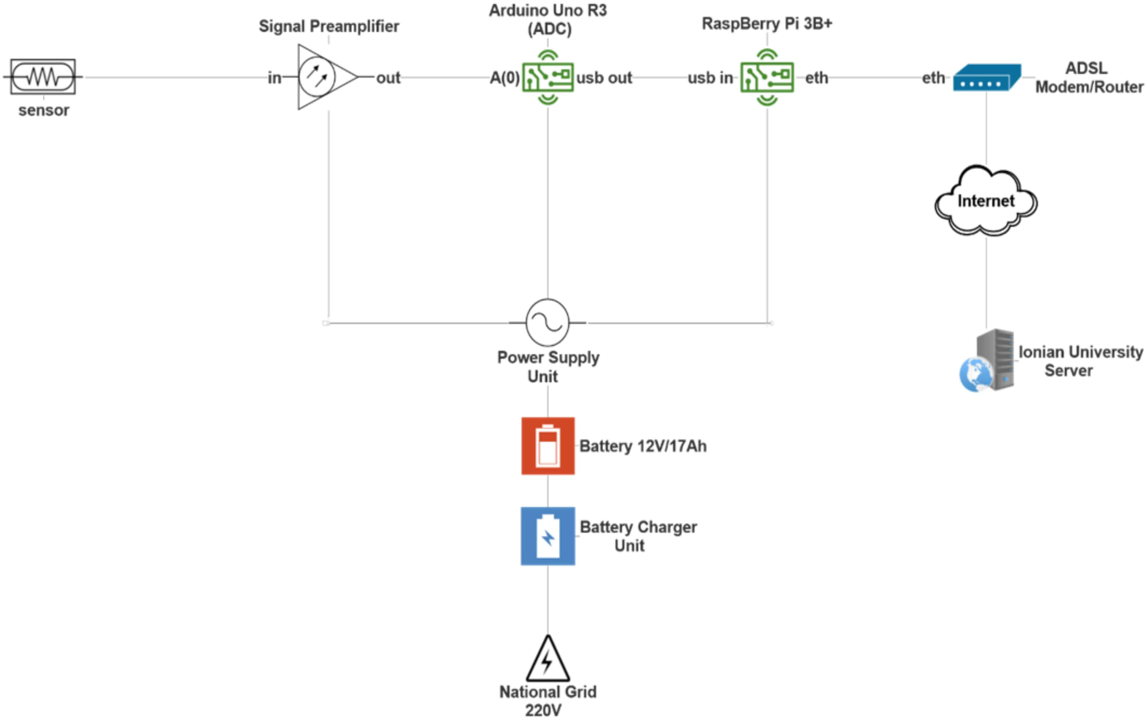

Data Acquisition and Seismograph Installation

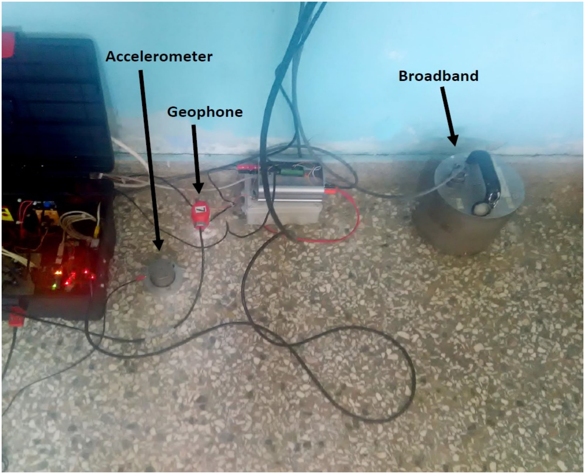
For the current study the Lefkada Island, and more specifically Evgiros, a settlement on the southeastern part of the island was chosen (Figure 6) because seismicity in the broader area is the highest in Greece.^25–27 In addition, seismicity is monitored by several permanent seismological stations with one of them in colocation with the low-cost seismic instruments. Thus, an adequate number of accurately located events, even of very low magnitude (M<1.0) are continuously recorded. The epicenters of the earthquakes of the last 10 years (2011–2020) have been plotted in Figure 6, using different colors and symbols which correspond to the magnitudes of earthquakes according to the map scale. The sites of the permanent seismological stations in Lefkada are also shown by brown hexagons. Considering that proper seismograph installation is of great importance when intending to avoid field noise,²⁸ both the classic broadband instrument and the low-cost seismographs were installed and are in operation on a bedrock founded floor of a non-working school in Evgiros (as seen on Figure 7). This site was selected in order for the instruments to be located far from human activities, external interference of power cables, vehicle traffic, or other devices that can produce electromagnetic interference. Furthermore, so as to avoid noise in the recorded signals, shielded cables were used for the connection between the sensors and their preamplifiers as well as from the preamplifiers to the analog-to-digital converters. Also, no interference from the power grid was observed in our recorded signals. Afterward, an earthquake catalog was compiled including twenty-eight (28) events which occurred in different epicentral distances (4–18.5 km) and with magnitudes in the range 1.4–3.3. These selected earthquakes were then divided and classified in terms of magnitude and distance. In more detail, Table 1 illustrates the seismic catalog with 28 events and their subdivision into three groups based on their magnitude (A, B, and C) along with six categories based on their epicentral distance (R1, R2, R3, R4, R5, and R6).

Figure 6.

Spatial distribution of seismic activity in the research area from 2011 to 2020. Brown hexagons represent the permanent seismological stations in Lefkada (including Evgiros).

Figure 7.

The three collocated sensors installed in Evgiros, in order to compare the seismic records between the conventional seismograph (broadband) and the low cost ones (accelerometer and geophone).

Table 1.

The earthquake catalog, which was used to compare results obtained by the conventional seismograph and the proposed low-cost one.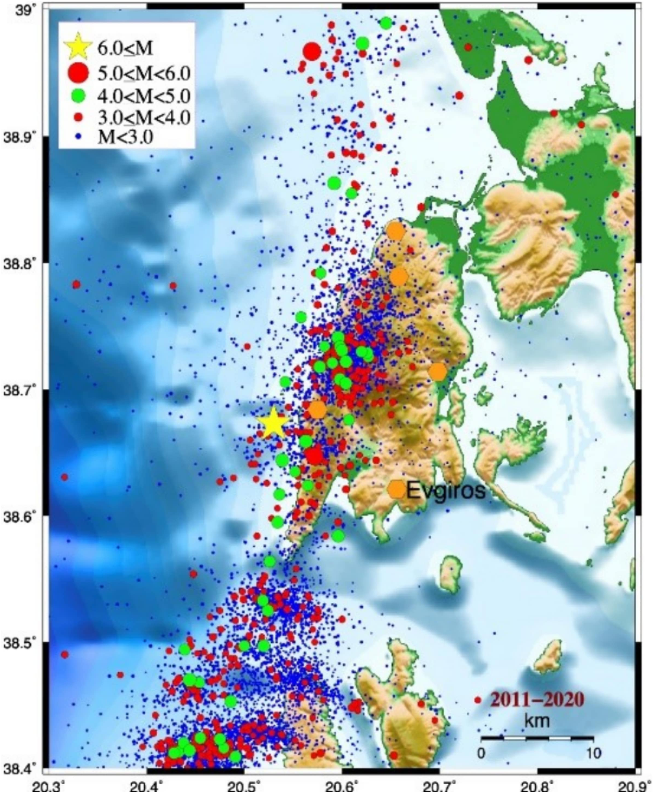

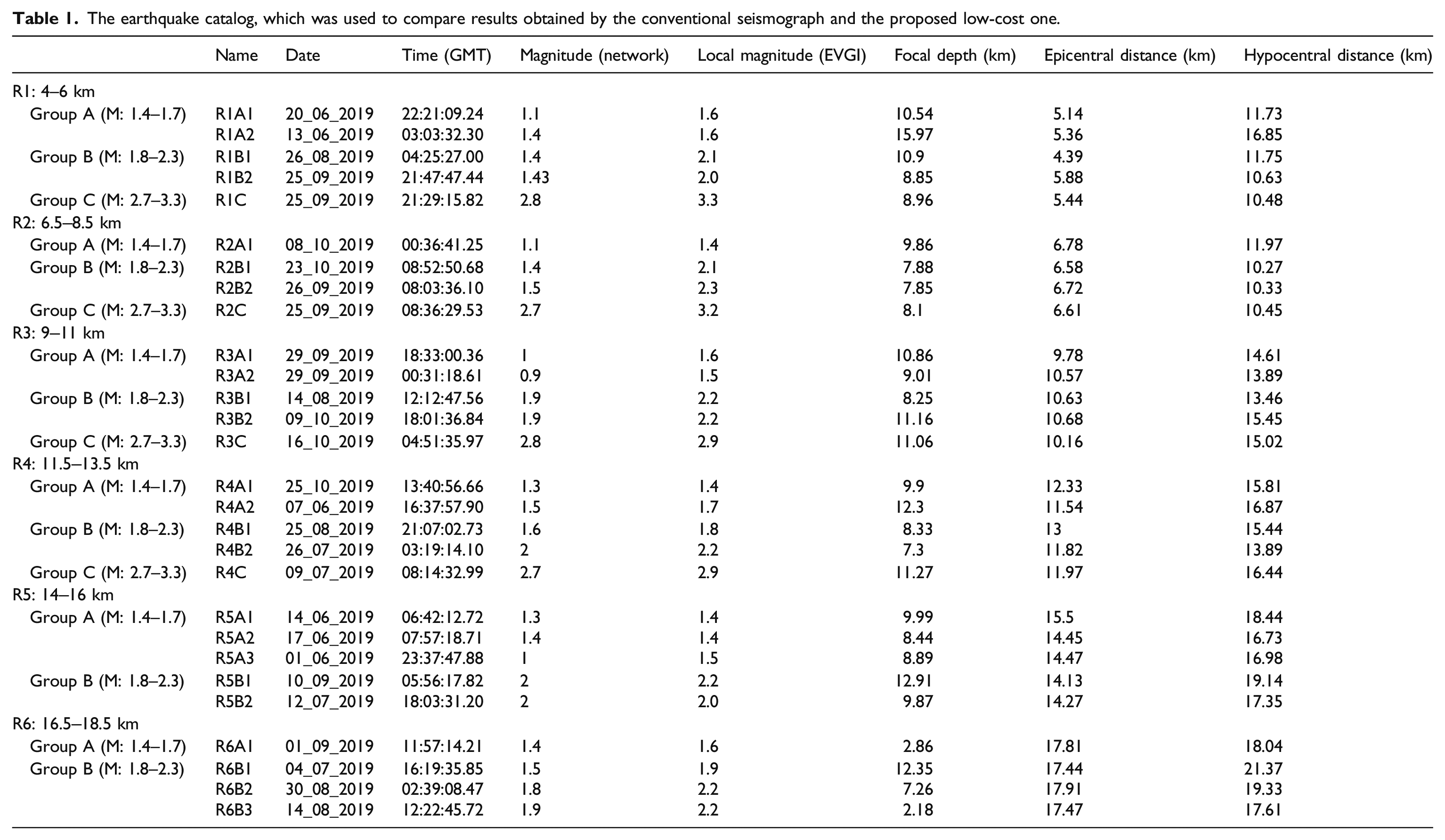
	Name	Date	Time (GMT)	Magnitude (network)	Local magnitude (EVGI)	Focal depth (km)	Epicentral distance (km)	Hypocentral distance (km)
R1: 4–6 km
Group A (M: 1.4–1.7)	R1A1	20_06_2019	22:21:09.24	1.1	1.6	10.54	5.14	11.73
Group A (M: 1.4–1.7)	R1A2	13_06_2019	03:03:32.30	1.4	1.6	15.97	5.36	16.85
Group B (M: 1.8–2.3)	R1B1	26_08_2019	04:25:27.00	1.4	2.1	10.9	4.39	11.75
Group B (M: 1.8–2.3)	R1B2	25_09_2019	21:47:47.44	1.43	2.0	8.85	5.88	10.63
Group C (M: 2.7–3.3)	R1C	25_09_2019	21:29:15.82	2.8	3.3	8.96	5.44	10.48
R2: 6.5‒8.5 km
Group A (M: 1.4–1.7)	R2A1	08_10_2019	00:36:41.25	1.1	1.4	9.86	6.78	11.97
Group B (M: 1.8–2.3)	R2B1	23_10_2019	08:52:50.68	1.4	2.1	7.88	6.58	10.27
Group B (M: 1.8–2.3)	R2B2	26_09_2019	08:03:36.10	1.5	2.3	7.85	6.72	10.33
Group C (M: 2.7–3.3)	R2C	25_09_2019	08:36:29.53	2.7	3.2	8.1	6.61	10.45
R3: 9‒11 km
Group A (M: 1.4–1.7)	R3A1	29_09_2019	18:33:00.36	1	1.6	10.86	9.78	14.61
Group A (M: 1.4–1.7)	R3A2	29_09_2019	00:31:18.61	0.9	1.5	9.01	10.57	13.89
Group B (M: 1.8–2.3)	R3B1	14_08_2019	12:12:47.56	1.9	2.2	8.25	10.63	13.46
Group B (M: 1.8–2.3)	R3B2	09_10_2019	18:01:36.84	1.9	2.2	11.16	10.68	15.45
Group C (M: 2.7–3.3)	R3C	16_10_2019	04:51:35.97	2.8	2.9	11.06	10.16	15.02
R4: 11.5‒13.5 km
Group A (M: 1.4–1.7)	R4A1	25_10_2019	13:40:56.66	1.3	1.4	9.9	12.33	15.81
Group A (M: 1.4–1.7)	R4A2	07_06_2019	16:37:57.90	1.5	1.7	12.3	11.54	16.87
Group B (M: 1.8–2.3)	R4B1	25_08_2019	21:07:02.73	1.6	1.8	8.33	13	15.44
Group B (M: 1.8–2.3)	R4B2	26_07_2019	03:19:14.10	2	2.2	7.3	11.82	13.89
Group C (M: 2.7–3.3)	R4C	09_07_2019	08:14:32.99	2.7	2.9	11.27	11.97	16.44
R5: 14‒16 km
Group A (M: 1.4–1.7)	R5A1	14_06_2019	06:42:12.72	1.3	1.4	9.99	15.5	18.44
	R5A2	17_06_2019	07:57:18.71	1.4	1.4	8.44	14.45	16.73
	R5A3	01_06_2019	23:37:47.88	1	1.5	8.89	14.47	16.98
Group B (M: 1.8–2.3)	R5B1	10_09_2019	05:56:17.82	2	2.2	12.91	14.13	19.14
Group B (M: 1.8–2.3)	R5B2	12_07_2019	18:03:31.20	2	2.0	9.87	14.27	17.35
R6: 16.5‒18.5 km
Group A (M: 1.4–1.7)	R6A1	01_09_2019	11:57:14.21	1.4	1.6	2.86	17.81	18.04
Group B (M: 1.8–2.3)	R6B1	04_07_2019	16:19:35.85	1.5	1.9	12.35	17.44	21.37
	R6B2	30_08_2019	02:39:08.47	1.8	2.2	7.26	17.91	19.33
	R6B3	14_08_2019	12:22:45.72	1.9	2.2	2.18	17.47	17.61

Group A consists of events with magnitudes ranging between 1.4 and 1.7 while the group B includes earthquakes with magnitudes ranging from 1.8 to 2.3. Group C encompasses four events with amplitudes between 2.7 and 3.3. A gap of magnitudes in the range between 2.3 and 2.7 is observed, which is due to the fact that during this monitoring period in this specific magnitude range, no events occurred.

Data analysis

This study was conducted using data derived from the proposed low-cost seismograph and the reference seismograph, which were freely available for download from the European Integrated Data Archive (EIDA) operated by the National Observatory of Athens (NOA), (http://eida.gein.noa.gr/). Since 2008, the Hellenic Unified Seismographic Network (HUSN) consisting of 259 seismological stations in total is in operation. In the Island of Lefkada, there are in operation five seismological stations maintained by the Geophysics Department of the Aristotle University of Thessaloniki in cooperation with the regional association of Ionian Islands municipalities (PED-IN). All the stations are equipped by 24-bit high resolution digitizers which are online connected with the Hellenic Unified Seismographic Network (HUSN). Three of them are equipped by short-period (1s-100 Hz) seismometers and the remaining two by broadband (30s-50 Hz) seismometers. For the timestamp, in UTC, a GPS receiver is used which continuously synchronizes the clocks of the system. The signal is digitized with a rate of 100 samples/second as in all the seismological stations of HUSN. All the 28 selected digital waveforms were requested and retrieved from Evgiros seismological station. All of them are shallow earthquakes with focal depths ranging between 1.6 km and 22.9 km. They occurred during the period June 2019–October 2019, in an area bounded by the parallels 38.5°- 38.9°N and the meridians, 20.3°-20.9°E (as seen in Figure 8).

Figure 8.

Regional map showing the study area along with all the 28 earthquakes selected from the initial seismic catalog (Table 1).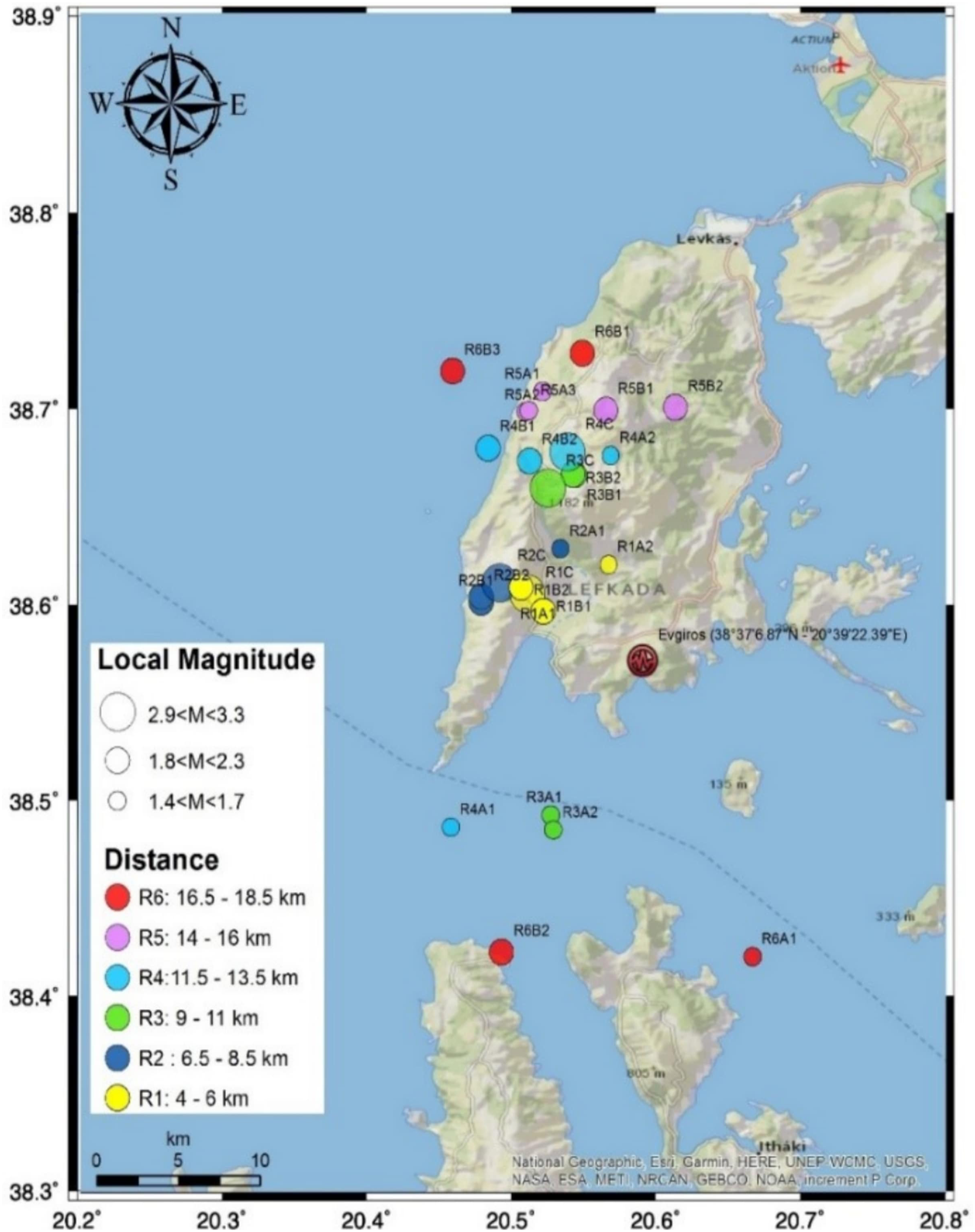

Having successfully chosen each event independently, all seismic waveforms were downloaded. Alongside for the same earthquakes, we searched in the Ionian University database and retrieved the corresponding 28 waveform files from the proposed low-cost seismograph. In this study, given that proposed systems sensors were single axis, we compared the vertical (Z) component, between the two systems. The real time clock of the proposed system uses local time of Greece (EET) for timestamp, which did not affect the general calculations at any point. After that, Mathworks Matlab software has been used for signal processing and analysis. The main objective was initially to analyze this set of the 28 events in terms of first arrival time estimation for the three seismographs.

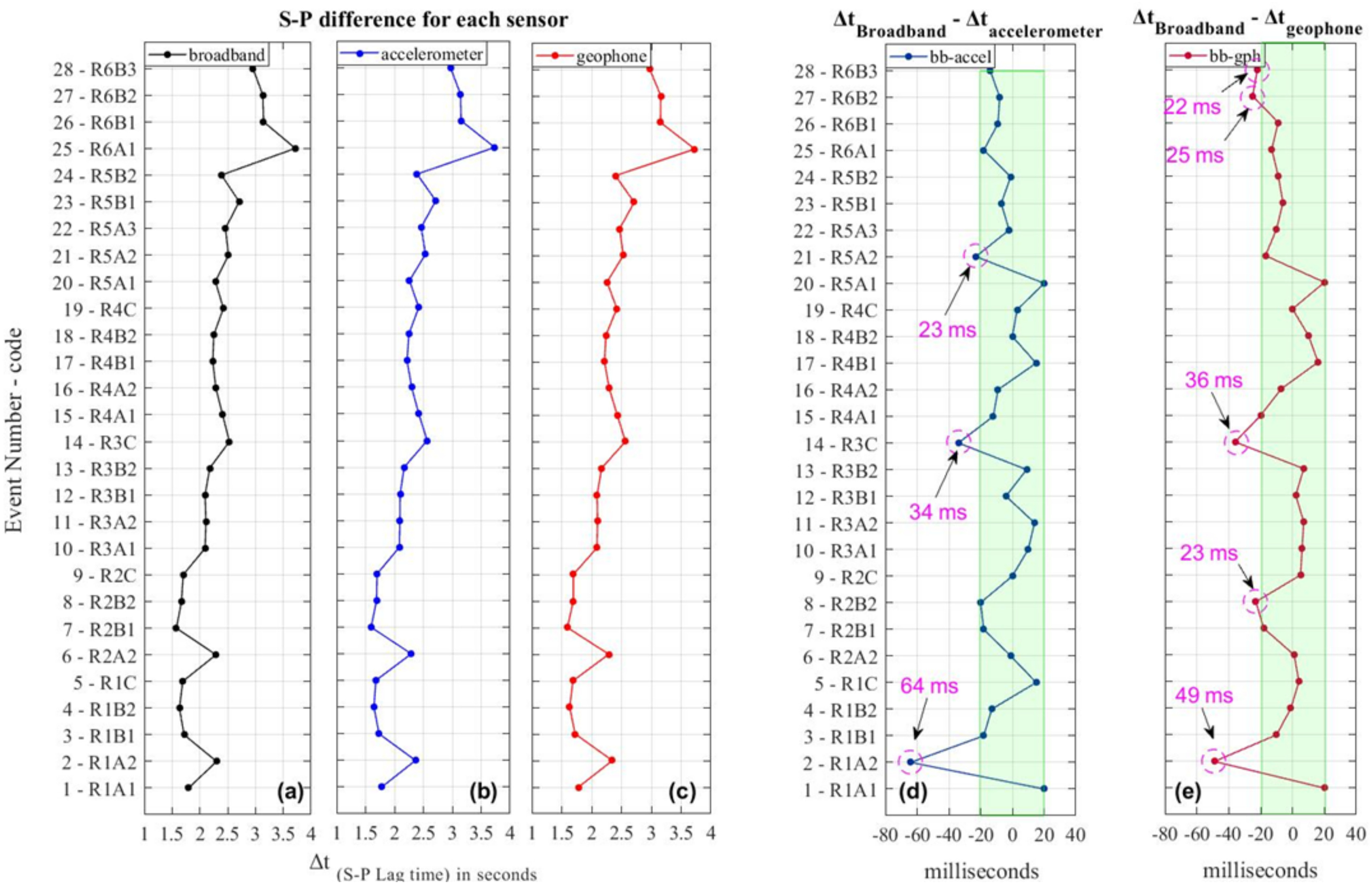
The analysis begins by plotting all seismic waveforms and accurately picking the arrival times for P and S waves. To better examine the signals belonging to the proposed system, they were plotted and projected together with the broadband ones along the 28 events. In all the seismograms (Figure 9), the green dashed line represents the P-wave arrival time for each sensor while the pink one the corresponding S-wave. We note that the broadband (black waveform) has significantly lower noise levels than the accelerometer (blue waveform) and geophone (red waveform), as expected. Despite the presence of noise in the low-cost systems seismograms, accurate first arrival identification was possible, as P and S waves were clearly recognizable. During the time period of these 28 analyzed events, no Internet connectivity loss occurred and as a consequence the results presented in Figure 9 had the maximum synchronization accuracy, as the timestamped data were continuously synchronized by Network Time Protocol (NTP) in real working conditions. Having completed this step, the S-P (Δt) difference was calculated in order to explore the capability of successful epicenter determination. Figure 10 depicts the S-P difference for each sensor, for all the earthquakes in the list (a: for accelerometer, b: for geophone, c: for broadband reference sensor). Next analysis step included the partial comparison for each event between the reference broadband sensor and the accelerometer and the reference broadband sensor with the geophone. Executing this procedure for the 28 events, two diagrams were produced. Figure 10(d) scrutinizes the Δt difference between broadband and accelerometer and Figure 10(e) the Δt difference between broadband and geophone. Considering a 20 millisecond-difference relatively tolerable (green shaded areas), the proposed seismograph showed satisfactory performance in determining first arrival times. The score value is referred to the percentage of events having Δt difference up to a certain level. The general score for the accelerometer was 89.29% and 85.71% for the geophone. The largest deviations were observed in events R1A2 and R3C with values 64 and 34 milliseconds for the accelerometer and 49 and 36 millisecond for the geophone. The remaining values outside the ± 20 millisecond-limit (event R5A2 for accelerometer and R2B2, R6B2, and R6B3 for geophone) are considered marginal, with values varying from 22 to 25 milliseconds.

Figure 9.

Indicative vertical component seismograms. Left: for the 25 September 2019, 21:47:47.44 GMT earthquake (event R1B2 - M_EVGI: 2.0, focal depth: 8.9 km). Right: Similarly for the 26 September 2019, 08:03:36.10 GMT earthquake (event R2B2 ‒ M_EVGI: 2.3, focal depth: 7.9 km). Upper part: Black waveforms for broadband sensor from the conventional high-cost seismograph (100 samples per second) - reference equipment. Middle: Blue waveforms for acceleration sensor, belonging to the proposed low-cost seismograph (345 sps). Lower part: Red waveforms for velocity sensor (geophone) from the proposed low-cost seismograph (345 sps).

Figure 10.

Calculated Δt (S-P) difference for each sensor for all the 28 events (a for broadband - reference sensor, b for accelerometer and c for geophone). Comparative plots showing the relative timing performance for the calculated Δt _broadband – Δt _{accelerometer} difference (d) and calculated Δt _broadband – Δt _geophone difference (e) for all the 28 events.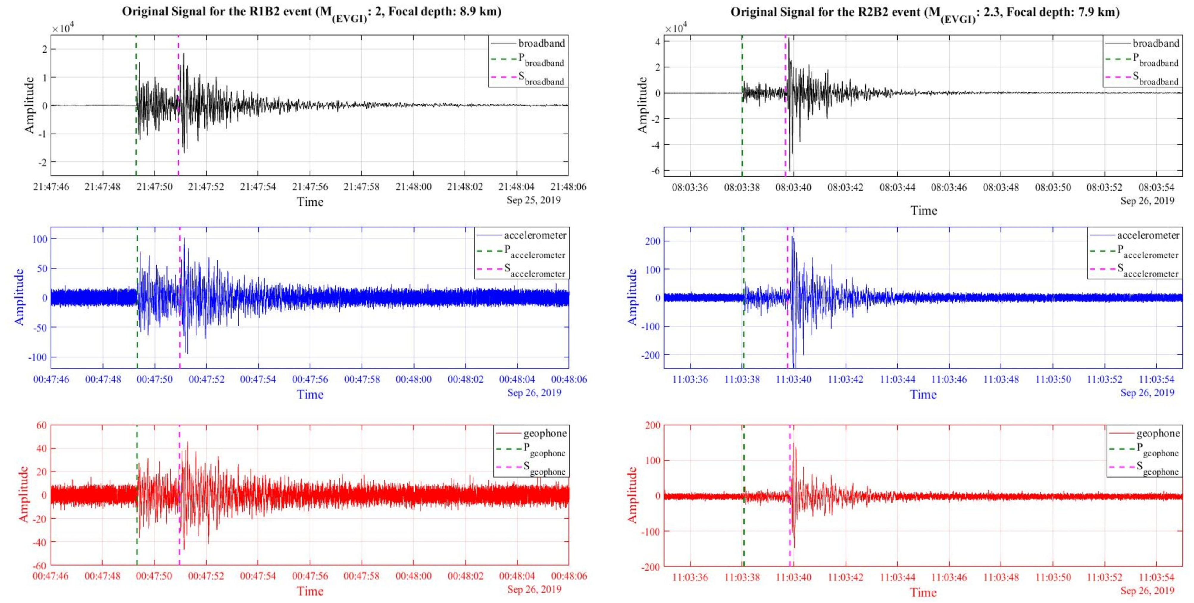

The second analysis stage included amplitude measurements together with magnitude calculation. Here, the basic approach was the accurate measurement of the zero to peak amplitudes for each sensor for all the 28 earthquakes. It should be stated that in absolute values, the broadband amplitudes were found some orders of magnitude higher than the accelerometers and the geophones, which was reasonable. Nevertheless, the current goal was whether the low-cost seismograph could sufficiently estimate the magnitude through a known relationship, including also the deviation from the reference magnitude values. With the intention of examining the efficiency of using epicentral or hypocentral distance we investigated two cases: (i) 0-peak amplitude with epicentral distance and (ii) 0-peak amplitude with hypocentral distance. In both approaches, magnitudes for accelerometer, geophone, and broadband were calculated. Taking into account that the under-analysis earthquakes occurred at close distances and focal depth is generally a difficult parameter to accurately be estimated, the selection and investigation of both distances appeared mandatory. Using the relation proposed by Scordilis et al. ²⁹ for reliable calculation of local magnitudes, and based on the already calculated magnitudes by the broadband seismometer, we calculated the parameter C_i for both the accelerometer and the geophone, as presented in equation (1):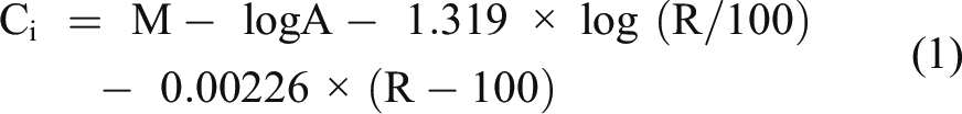

C_{i} = M - logA - 1 .319 × \log (R /100) - 0 .00226 × (R - 100)

(1)

R1A1-accelerometer, R1A1-geophone R1A1-broadband M denotes the local magnitude from EVGI seismological station (M_EVGI), logA the logarithm of zero-to-peak amplitude, and R the distance (case i: epicentral distance, case ii: hypocentral distance). Repeating this procedure for all the earthquakes, the mean value C_{i_avg} was acquired, for each sensor separately, as seen on Table 2. The above process was applied for both the epicentral (case i), and the hypocentral distance (case ii).

Table 2.

Calculated C_{i_avg} values for each sensor as the mean of the 28 C_i values, for both epicentral and hypocentral distances (cases i and ii).

	Epicentral distance (case i)	Hypocentral distance (case ii)
C_{i_avg} for accelerometer	1.625	1.322
C_{i_avg} for geophone	1.850	1.630
C_{i_avg} for broadband	−0.665	−0.886

Incorporating C_{i_avg} in equation (1) and solving with respect to Μ, it is derived that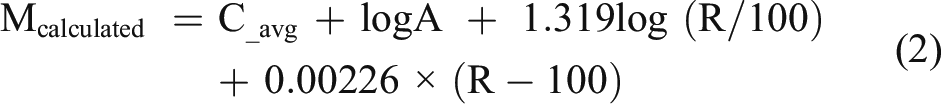

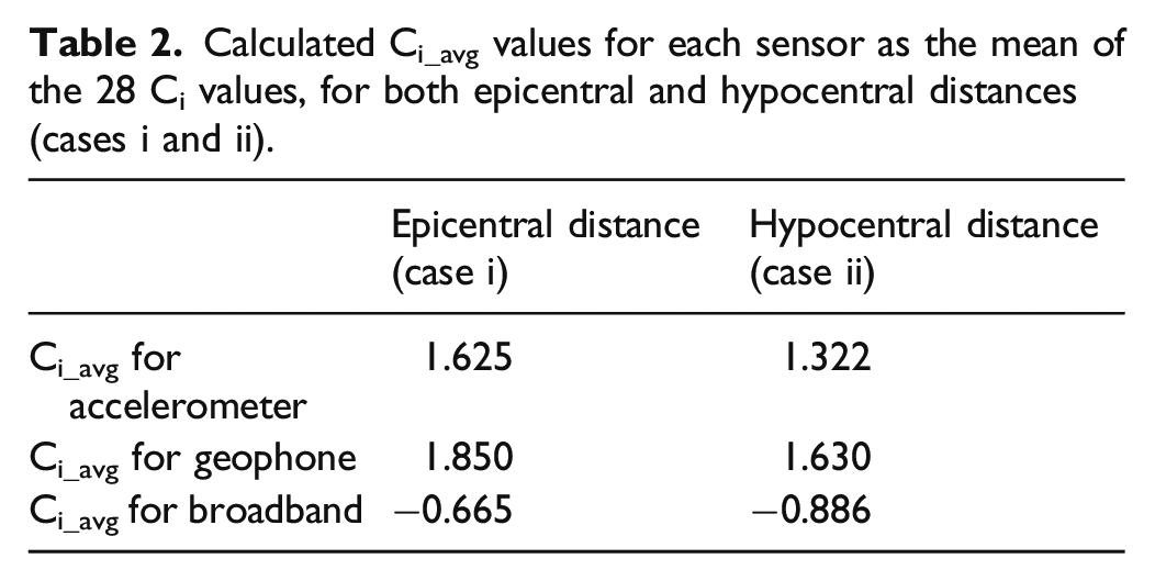
M_{calculated} = C_{_avg} + logA + 1 .319log (R /100) + 0 .00226 × (R - 100)

(2)

This process was executed for all the events of the seismic catalog (equation (2)), to obtain the calculated magnitude values (M_calculated), for both epicentral (case i) and hypocentral (case ii) distances. Figure 11 depicts the relationship between the local calculated magnitudes per sensor (on y-axis) and the reference local magnitudes of the broadband seismometer (EVGI) (x-axis). In order to examine whether the proposed low-cost seismograph estimates are reliable, the correlation coefficient (R ²) values of all magnitude calculations were obtained. In addition, the M_EVGI – M_calculated difference for each sensor was then used to construct histograms of their distribution with a bin size of 0.2. The correlation coefficient (R ²) values for the broadband seismometer were close to one (0.95 for hypocentral and 0.91 for epicentral distance), with a standard deviation of 0.13 (case ii—hypocentral distance) and 0.16 (case i—epicentral distance), evidencing the reliability of the calculated magnitudes. As far as the low-cost system is concerned, starting with the hypocentral distance, the correlation coefficient (R ²) for accelerometer was 0.77 and for the geophone was 0.80. Moreover, as for the standard deviation values, they were calculated 0.31 and 0.27 for the accelerometer and the geophone, respectively. The epicentral distance gave moderate correlation values, equal to 0.59 for accelerometer and 0.71 for the geophone, while standard deviations were 0.35 and 0.31, respectively, indicating larger deviations in the calculated quantities between the two recording systems. We observe that through equation (2), reliable magnitude estimation becomes possible and more specifically, using the hypocentral distance, quite similar results are acquired.

Figure 11.

Local magnitudes estimated by equation (2) versus reference local magnitudes for EVGI seismological station, along with their correlation coefficients, for epicentral distance (a). Black points (on the left) correspond to broadband, blue points (in the middle) to accelerometer and finally red points (on the right) are associated to geophone. Frequency distribution of the derived M_EVGI - M_calculated values along with their standard deviation, for epicentral distance (b). Black bins (on the left) are associated to broadband, blue bins (in the middle) correspond to the accelerometer and finally red bins (on the right) correspond to the geophone. (c): Similar to (a) for hypocentral distance. (d): Similar to (b) for hypocentral distance.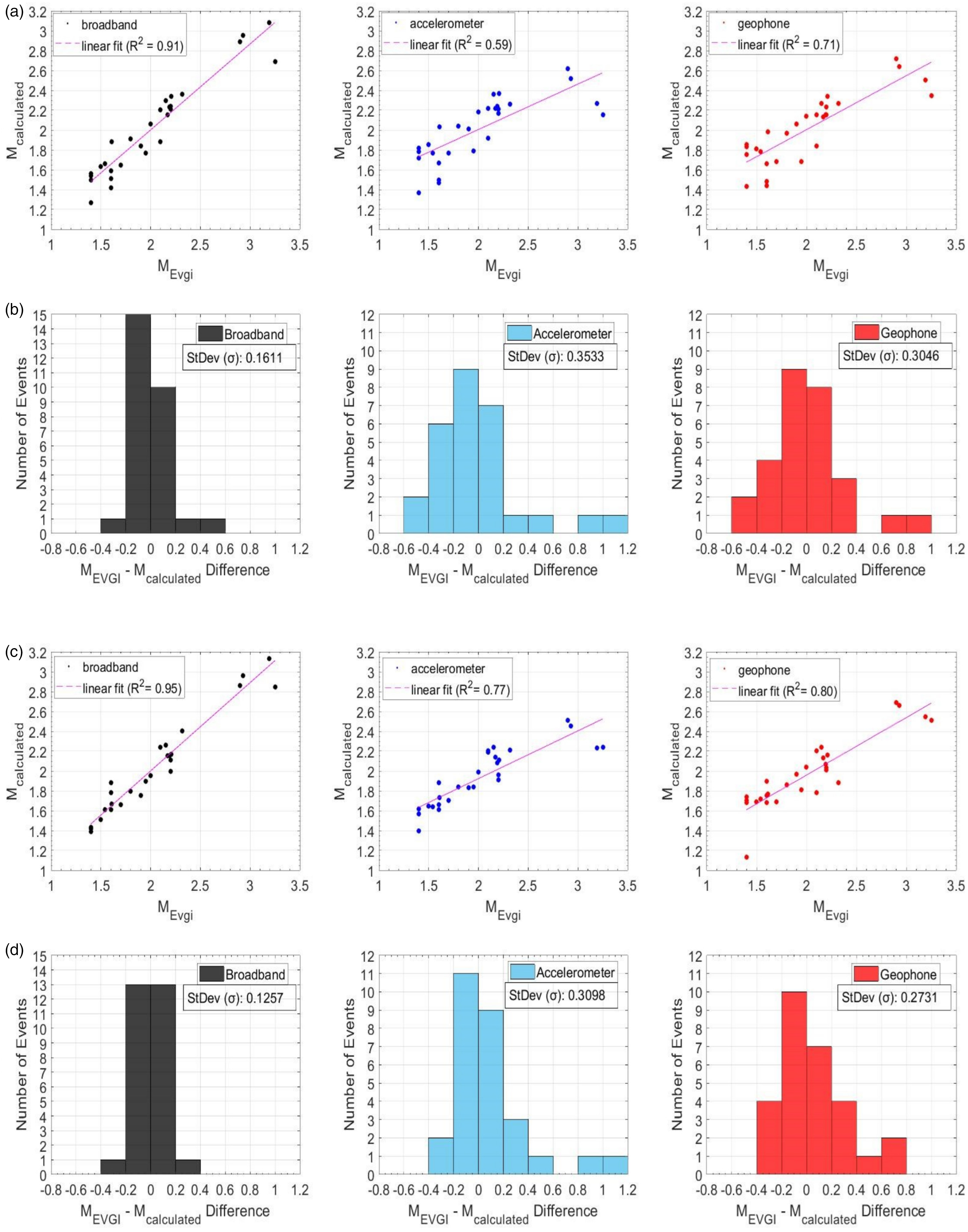

To better determine the magnitude performance between the two systems, the calculated magnitudes of accelerometer and geophone were further compared not only against the reference local magnitudes for EVGI seismological station, but also against the broadband seismometer calculated magnitudes. This way, using Scordilis equation (relationship 2), we were able to illustrate the variations in magnitude calculation between the three sensors. Figure 12 highlights this reasonable efficiency where the correlation coefficient (R ²) for accelerometer was 0.81 for epicentral distance and 0.86 for hypocentral distance, while the correlation coefficient (R ²) for geophone was 0.90 for epicentral distance and 0.81 for hypocentral distance. In epicentral distance, the geophone showed more efficient behavior in magnitude calculation than the accelerometer. On the other hand, the accelerometer showed more efficient behavior in magnitude calculation than the geophone in hypocentral distance. Including more earthquakes in the next research stages, undoubtedly, it can be ascertained which of the two distances is the most appropriate to use.

Figure 12.

Calculated local magnitudes from the low-cost systems sensors versus calculated local magnitudes from the reference seismographs sensor (broadband), along with their correlation coefficient R ². (Left part is referred to the accelerometer and the right part for geophone, upper part: epicentral distance – lower part: hypocentral distance).

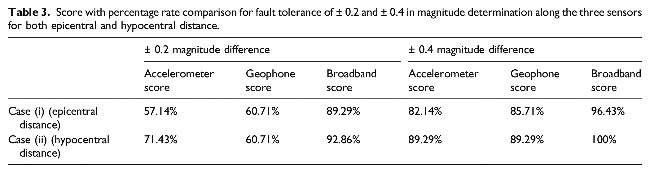
The dependence of the M_EVGI – M_calculated magnitude differences along with the distance is examined in Figure 13, which is identical to Figure 11(a) and Figure 11(c) but adjusted to provide the additional distance information. It is important to note that the bigger misfits are observed at close distances (4–8.5 km) and large magnitudes and more specific for events R1C and R2C of the initial seismic catalog. Starting with event R1C (_MEVGI: 3.3) and epicentral distance (Figure 13—upper part), the M_EVGI – M_calculated difference was found equal to 1.1 for the accelerometer, 0.9 for the geophone and 0.6 for broadband. For R2C event (M_EVGI: 3.2), the M_EVGI – M_calculated difference was measured to 0.9 for the accelerometer, 0.7 for the geophone and 0.1 for broadband. As for the hypocentral distance (Figure 13—lower part), the M_EVGI – M_calculated difference for event R1C was slightly reduced to 1 for accelerometer, 0.7 for geophone, and 0.4 for broadband. Subsequently, for event R2C was 1 for accelerometer, 0.6 for geophone, and 0.1 for broadband. In conclusion, these two events form marginal cases, as the magnitude deviation was higher than 1.

Figure 13.

Comparison between calculated magnitude misfits along with their distance information for the three sensors (black dots for broadband, blue dots for accelerometer and red ones for geophone). Upper part for epicentral distance and lower part for hypocentral distance.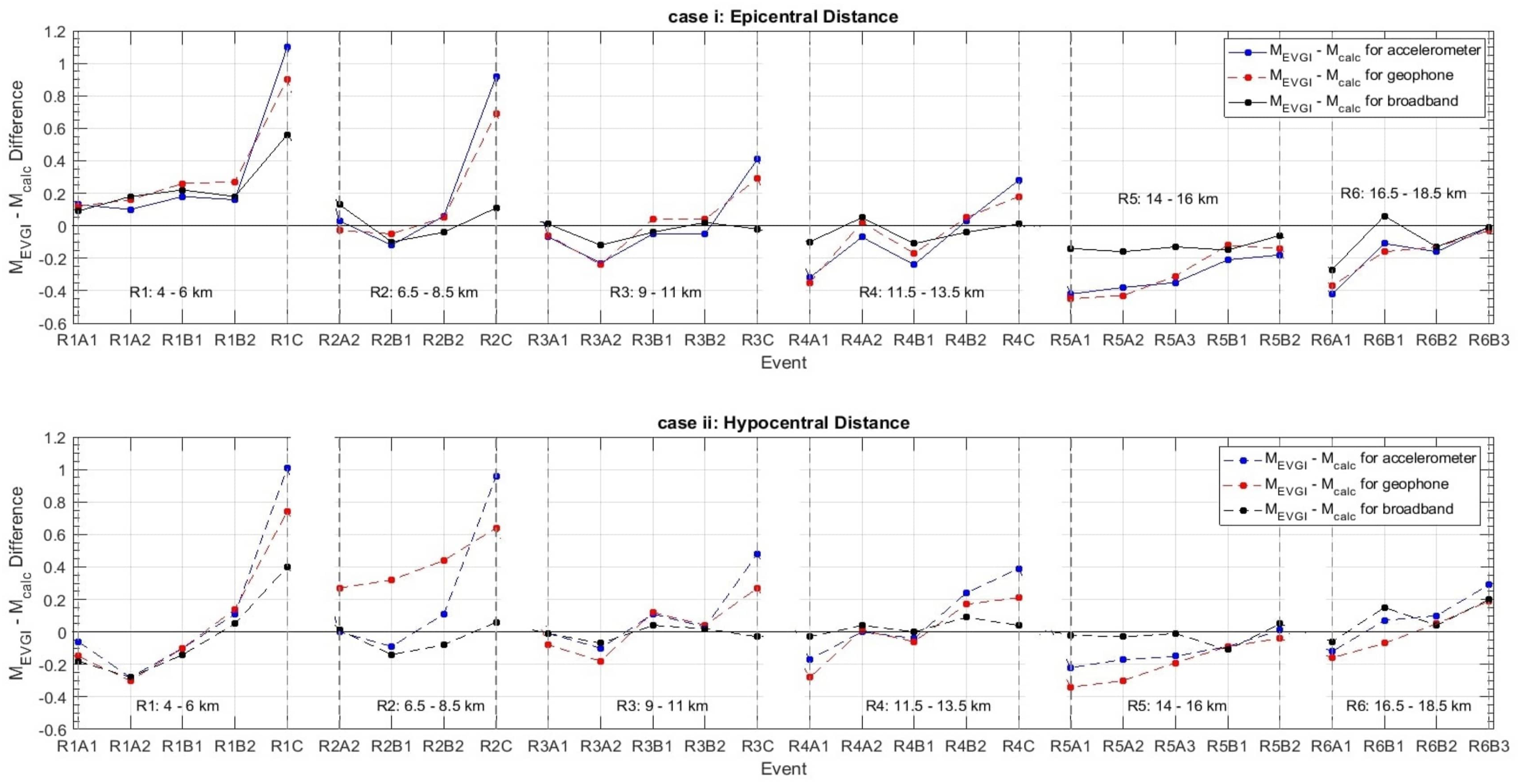

In order to present a more evident understanding of the magnitude differences shown in Figure 13, Table 3 presents a comparison between the scores for difference ± 0.2 and difference ± 0.4. The score value is referred to the percentage of events having magnitude difference up to a certain level. The broadband scores are currently presented as reference point. Relatively to ± 0.2 difference in calculated magnitudes, for the accelerometer, the score values range from 57.17% for epicentral distance to 71.43% for hypocentral distance. Meanwhile, the score values are equal to 60.71% for both distances for geophone. Additionally, the broadband scores are found almost similar: 89.29% for epicentral distance and 92.86% for hypocentral distance. However, the above scores from the low-cost system are significantly improved for ± 0.4 difference: 82.14% and 85.71% for accelerometer and geophone for epicentral distance and 89.29% for accelerometer and geophone, respectively, for hypocentral distance. Broadband achieved 96.43% for epicentral and 100% for hypocentral distance. These final results clearly indicate that, almost precise and reliable magnitude determination can be attained, when a error tolerance of ± 0.4 is chosen.

Table 3.

Score with percentage rate comparison for fault tolerance of ± 0.2 and ± 0.4 in magnitude determination along the three sensors for both epicentral and hypocentral distance.

	± 0.2 magnitude difference			± 0.4 magnitude difference
	Accelerometer score	Geophone score	Broadband score	Accelerometer score	Geophone score	Broadband score
Case (i) (epicentral distance)	57.14%	60.71%	89.29%	82.14%	85.71%	96.43%
Case (ii) (hypocentral distance)	71.43%	60.71%	92.86%	89.29%	89.29%	100%

The third analysis stage encloses spectral investigation for all the systems by means of Fast Fourier Transform (FFT).³⁰ Initially, in order to confirm that the signal response of the 4.5 Hz geophone sensor used was not affected from its non-linear response region, the spectral content of the ground velocity for all the 28 events was calculated using the recordings of the broadband sensor. In all cases, the corner frequencies are traced considerably above the linear frequency response threshold of the geophone (4.5 Hz) and the accelerometer (0.4 Hz). Figure 14(a) shows the 12 July 2019, 17:59:58.855 GMT earthquake (event R5B2—M_EVGI: 2—focal depth: 9.9 km) while Figure 14(b) depicts the 29 September 2019, 18:29:57.395 GMT earthquake (event R5B2—MEVGI: 1.6—focal depth: 10.9 km). Following the previous description, Figure 14(c) presents the spectral content for the 26 August 2019, 04:24:59.745 GMT earthquake (event R1B1—M_EVGI: 2, focal depth: 8.9 km) and Figure 14(d) shows the spectral content for the 25 September 2019, 08:34:58.315 GMT earthquake (event R2C—M_EVGI: 3.2, focal depth: 8.1 km).

Figure 14.

Examples of the ground velocity frequency content of the events recorded by the broadband reference sensor (100sps) calculated by means of the Fast Fourier Transform. (a) Indicative frequency representation of the 12 July 2019, 17:59:58.855 GMT earthquake (event R5B2 - M_EVGI: 2.0, focal depth: 9.9 km) (b) frequency representation of the 29 September 2019, 18:29:57.395 GMT earthquake (event R3A1 - M_EVGI: 1.6, focal depth: 10.9 km) (c), the 26 August 2019, 04:24:59.745 GMT earthquake (event R1B1 ‒ M_EVGI: 2, focal depth: 8.9 km) and (d) indicative frequency representation for the 25 September 2019, 08:34:58.315 GMT earthquake (event R2C ‒ M_EVGI: 3.2, focal depth: 8.1 km).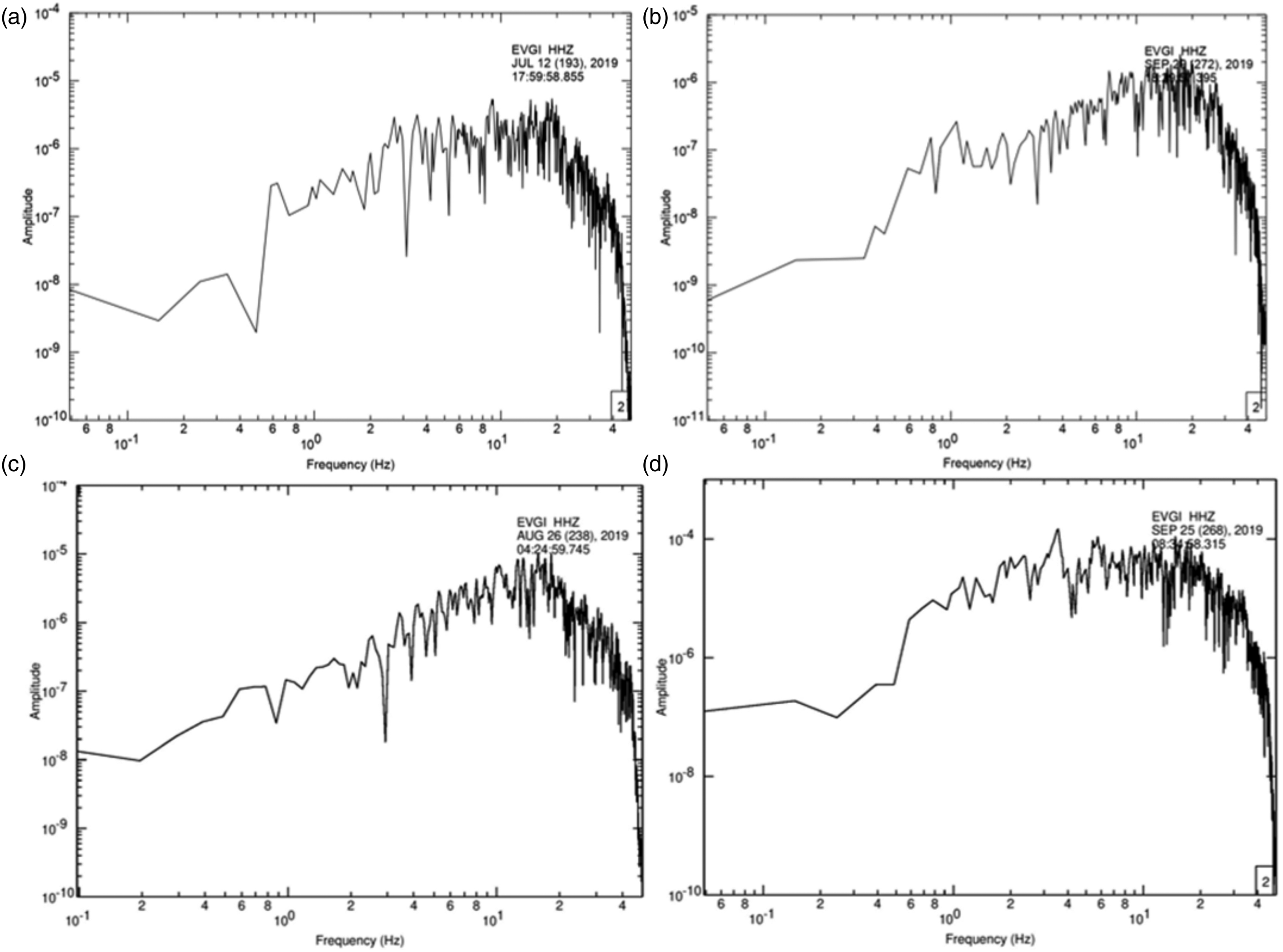

The frequency distribution of the 25 September 2019, 21:47:47.44 GMT earthquake (event R1B2—M_EVGI: 2—focal depth: 8.9 km) is depicted in Figure 15(a). Similarly, Figure 15(b) shows the frequency distribution of the 26 September 2019, 04:25:27 GMT earthquake (event R2B2—M_EVGI: 2.3, focal depth: 7.8 km). In both cases, blue and red waveforms are referred to the accelerometer and the geophone, respectively, (345 samples per second). On the other hand, the black waveform represents the reference FFT distribution system from the conventional high-cost seismograph (100 samples per second). It is noted that the broadband amplitudes have significantly higher levels (max_R1B2 event: 370.3, max_R2B2 event: 852.3) than the accelerometer (max_R1B2 event: 1.82, max_R2B2 event: 4.93) and the geophone ones (max_R1B2 event: 1.02, max_R2B2 event: 2.72). In order to obtain the relative frequency deviation among the systems, amplitude normalization on y-axis was applied.

Figure 15.

Indicative amplitude versus frequency curves of the 25 September 2019, 21:47:47.44 GMT earthquake (event R1B2 - M_EVGI: 2, focal depth: 8.9 km) (a) and for the 26 September 2019, 08:03:36.10 GMT earthquake (event R2B2 - MEVGI: 2.3, focal depth: 7.9 km) (b). The blue waveforms refer to the accelerometer and the red ones to the geophone, both belonging to the proposed low-cost seismograph (345sps). On the other hand, the black waveforms represent the reference sensor (broadband) from the conventional high-cost seismograph (100sps). Left side: Logarithmic amplitude spectrum – frequency plot with all sensors. Right side: Y-axis-normalized FFT representation (amplitude over frequency) along with their 0.99 smoothing constant for the three sensors.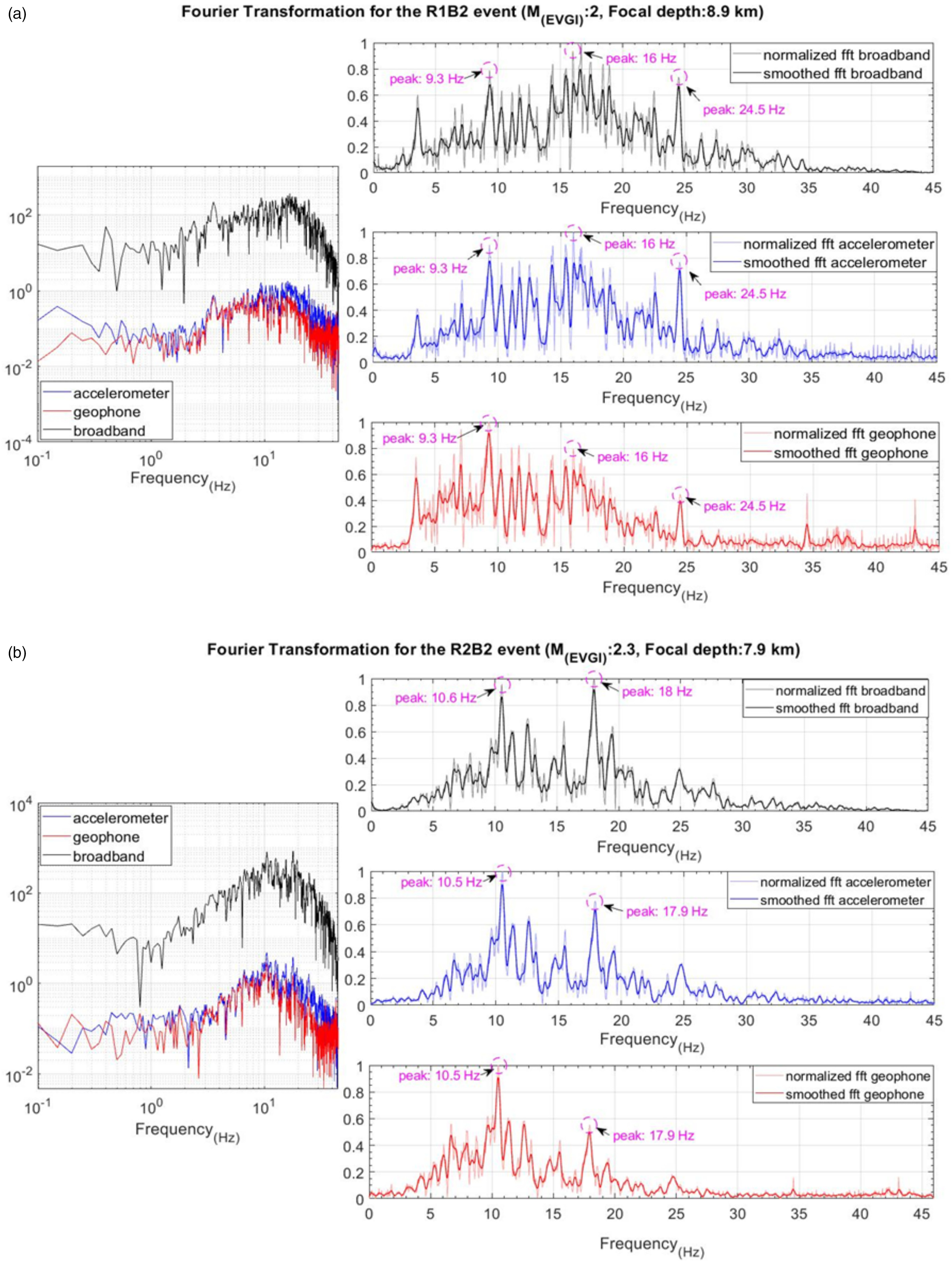

Then, smoothing process was performed for noise attenuation. These normalized diagrams are shown together with their corresponding 0.99 smoothing constant, as shown Figure 15(a) and Figure 15(b) (right part). A significant similarity is observed. More specific, the frequency content has a major increase between 0 Hz and 25 Hz, with represented peaks at 9.3 Hz, 16 Hz, and 24.5 Hz for R1B2 event and 10.6 Hz and 18 Hz for R2B2 event. From this point onwards, frequency values show a constant diminution until 45 Hz. Although the gain of broadband is much higher than the corresponding accelerometer and geophone, the normalized relative frequency distribution is similar. In general, accelerometer tends to show a better shape similarity. Moreover, it establishes a more tolerant behavior and approaches the same frequency peaks as the broadband.

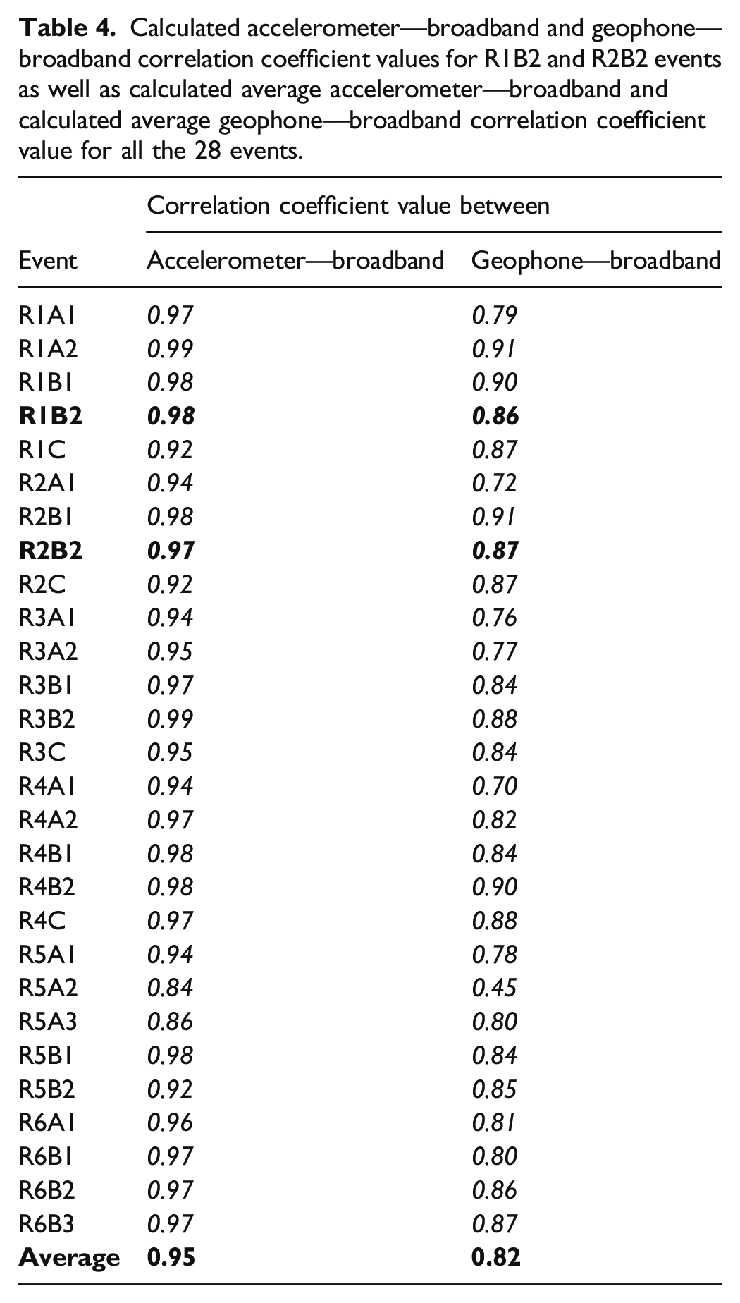
In order to explore the total energy distribution, the area under the smoothed normalized FFT signals was chosen for further analysis. As a consequence, we performed a numerical integration via the trapezoidal method for each sensor with a step of 1 Hz for all the 28 events of the seismic catalog.³¹ Taking into account the above computations, the emerged results concerning R1B2 and R2B2 event are presented in Figure 16(a) and Figure 16(b), respectively (left part). These results highly reveal an adequate agreement between the three sensors, as important waveform similarities are identified in the energy curves. The larger energy distribution proportionally to the FFT curves, is allocated in the frequency area between 0 Hz and 25 Hz, with indicative peaks of released energy at 9.5 Hz, 10.5 Hz, and 16.5 Hz. This tendency was also observed in the remaining 26 events. Aiming to quantify the validation of spectral data, a statistical analysis for all the 28 events has been performed. Intending to compare the similarity between the waveforms of the proposed seismograph and the reference one, the cross-correlation function was used, in order to obtain the correlation coefficient as a value of similarity. The correlation coefficient values concerning R1B2 and R2B2 events between the accelerometer and broadband, as well as between the geophone and broadband, respectively, are presented in Figure 16(a) and Figure 16(b) (right part). For all the 28 events, a great similarity between the energy over frequency waveforms of proposed seismograph and the conventional ones has been revealed. The average correlation coefficient values between the accelerometer and broadband were 0.95, while between the geophone and broadband were 0.82, as presented in Table 4. Moreover, comparing the sensors of the proposed low-cost systems, the accelerometer established a more acceptable functionality than the geophone.

Figure 16.

Left side: 1 Hz - step relative energy over frequency plots originating from the Y-axis-normalized FFT plots for the three sensors of the 25 September 2019, 21:47:47.44 GMT earthquake (event R1B2 ‒ M_EVGI: 2, focal depth: 8.9 km). Right side: Accelerometer to Broadband and Geophone to Broadband waveform similarity investigation, using the correlation coefficient value. (a) Similarly to (a), 1 Hz ‒ step relative energy over frequency plots originating from the Y-axis-normalized FFT plots for the three sensors for the 26 September 2019, 08:03:36.10 GMT earthquake (event R2B2 ‒ M_EVGI: 2.3, focal depth: 7.9 km) (b).

Table 4.

Calculated accelerometer—broadband and geophone—broadband correlation coefficient values for R1B2 and R2B2 events as well as calculated average accelerometer—broadband and calculated average geophone—broadband correlation coefficient value for all the 28 events.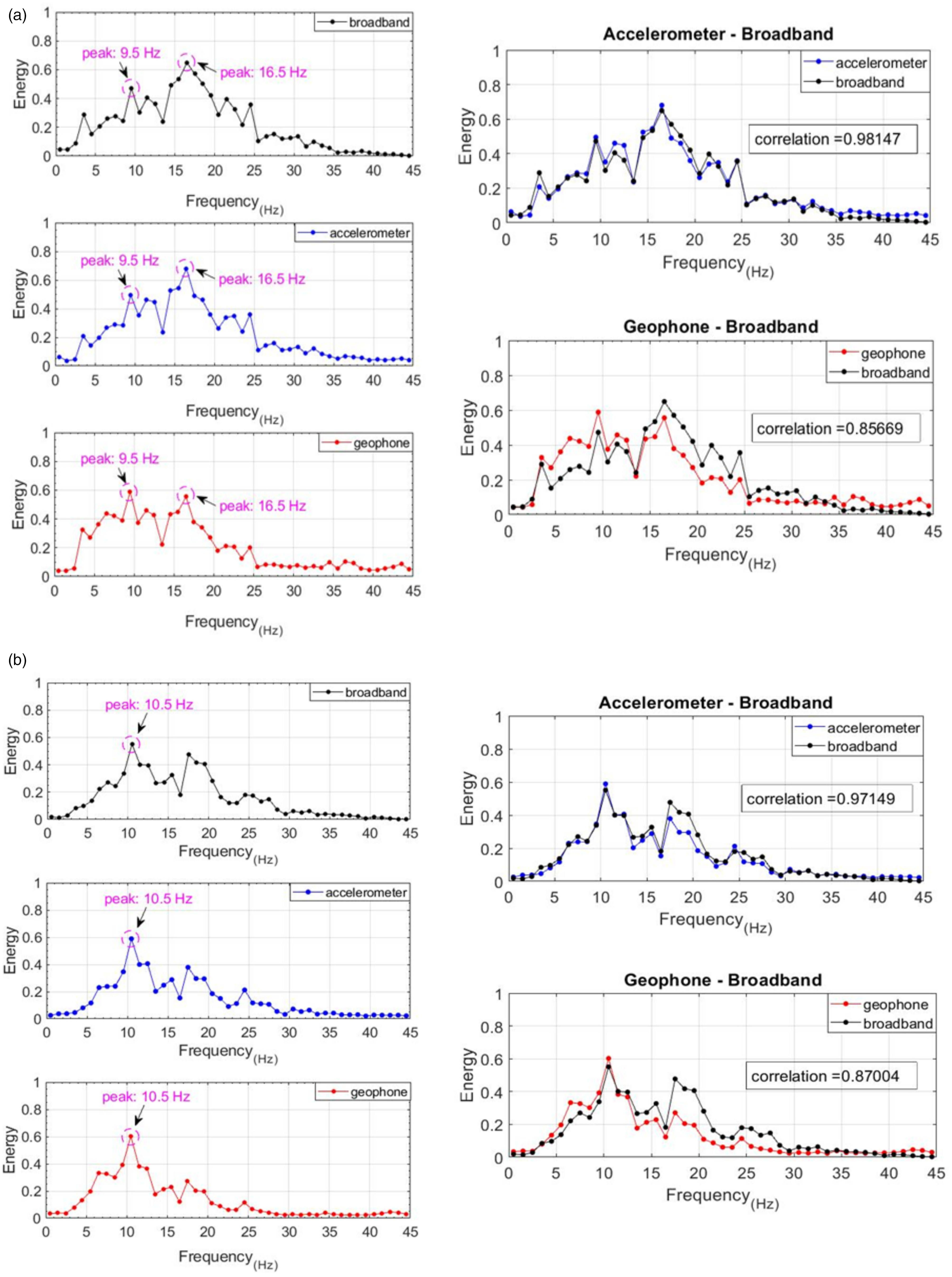

Event	Correlation coefficient value between
Event	Accelerometer—broadband	Geophone—broadband
R1A1	0.97	0.79
R1A2	0.99	0.91
R1B1	0.98	0.90
R1B2	0.98	0.86
R1C	0.92	0.87
R2A1	0.94	0.72
R2B1	0.98	0.91
R2B2	0.97	0.87
R2C	0.92	0.87
R3A1	0.94	0.76
R3A2	0.95	0.77
R3B1	0.97	0.84
R3B2	0.99	0.88
R3C	0.95	0.84
R4A1	0.94	0.70
R4A2	0.97	0.82
R4B1	0.98	0.84
R4B2	0.98	0.90
R4C	0.97	0.88
R5A1	0.94	0.78
R5A2	0.84	0.45
R5A3	0.86	0.80
R5B1	0.98	0.84
R5B2	0.92	0.85
R6A1	0.96	0.81
R6B1	0.97	0.80
R6B2	0.97	0.86
R6B3	0.97	0.87
Average	0.95	0.82

Conclusions

Herein, we present a low-cost seismograph which was designed to improve local seismicity monitoring through a dense seismic network. This cost-competitive device which includes a version with velocity sensor as well as one with acceleration sensor, was installed together with a high-cost seismograph (broadband sensor) on a region of high seismicity on Evgiros, Lefkada Island, Greece. The novelty of the proposed system is that it is based on IoT technology, incorporating two common sensors (a 4.5 Hz vertical geophone and a ceramic high sensitivity accelerometer) along with a microcontroller and a microprocessor board. For a period of 18 months, raw seismic data have been recorded, remotely transferred and stored to the Ionian University database for further analysis. The aim of this research was the comparison of the seismic records between the proposed low-cost devices and the conventional seismograph, in order to assess whether they can be used for reliable earthquake monitoring. Digital records of Evgiros seismological station were used to conduct this study. A set of 28 earthquakes with magnitudes between 1.4 and 3.3 was analyzed in terms of timing accuracy, magnitude, and frequency. Preliminary results indicate satisfactory sensitivity tolerance for local events within a radius which not exceed 18.5 km. An overall agreement was found for P and S arrival time estimation between the devices, as depicted in Figure 9 for 20 millisecond deviation tolerance. The largest deviations were only observed on 13th June 2019, 03:03:32.30 GMT earthquake (event R1A2—M_EVGI: 1.6, focal depth: 15.97 km) and on 16th October 2019, 04:51:35.97 GMT earthquake (event R3C—M_EVGI: 2.9, focal depth: 11.06 km). After all, both the accelerometer and geophone warranted a precise and trustworthy estimation of arrival times. Regarding the magnitude calculation, the analysis results showed that using equation (2), the proposed low-cost systems are capable of determining every new earthquake’s magnitude with a ± 0.4 difference (Table 3). Taking the last into account, the proposed systems constitute a reasonable choice in magnitude determination. The largest deviations were observed at higher magnitudes, in Group C events of the initial seismic catalog. At this point, the more efficient behavior of the geophone against the accelerometer in magnitude calculation in epicentral distance, should be declared. Moreover, as far as spectral investigation is concerned, the broadband amplitudes in the FFT graphs had significantly larger levels than the accelerometer and geophone ones, as expected. Aiming to increase the discrimination capability of the low-cost seismographs, amplitude normalization on y-axis was performed, highlighting an identical frequency distribution. The majority of events indicated a significant increase in the frequency content between 0 Hz and 25 Hz as well as a smooth and gradually decrease from 25 Hz to 45 Hz. Furthermore, using a numerical integration via the trapezoidal method in the abovementioned FFT graphs, the relative energy distribution with a 1 Hz step for all the 28 events was determined. The relative energy content similarity between the instruments was indicative, demonstrating the alternative use of the proposed seismograph. Furthermore, another situation of particular importance here is that the accelerometer established a more tolerant behavior than the geophone, as in terms of frequency distribution, it almost approached the same frequency peaks as the broadband did.

The results up to this point are very promising and the advantages of proposed seismograph can be further improved by upgrading the current 10-bit A/D converter with a new one of 24 bit as well as by integrating a GPS circuit for even greater timestamp accuracy of the recorded signals. In addition to those hardware improvements, the next research stages will include more earthquake integration to create an extended test list. The later will reveal which of the two distances between the epicentral and the hypocentral can give the least possible deviations and is more appropriate for use. Another important factor of consideration should be the inclusion and processing of events with magnitudes higher than 3.3 and less than 1.4, filling the gap in the current seismic catalog. The underlying goal of the current research is to develop reliable low-cost acquisition devices that will cost less than the ordinary seismological stations, while they will provide the necessary acceptable accuracy for effective seismicity monitoring. Nonetheless, our final target is not to compare and replace the high-cost seismograph with the proposed, one by one, as it is clearly not possible to receive all the seismic information extracted from conventional instruments with a single low-cost unit. However, it is more realistic to gain as much signal information as possible, both in time and frequency domain, as a satisfactory amount of this abovementioned valuable information can be extracted through a dense monitoring network of the designed low-cost seismographs. In their final form, the proposed cost competitive seismographs will be able, through a dense monitoring network, to reliably detect first arrival times, calculate the magnitude as well as to investigate spectral content of the recorded seismic activity.

Supplemental Material

sj-pdf-1-mac-10.1177_00202940211064448 – Supplemental Material for Data-driven performance evaluation of a low-cost seismograph

Supplemental Material, sj-pdf-1-mac-10.1177_00202940211064448 for Data-driven performance evaluation of a low-cost seismograph by Spiridon G Krokidis, Ioannis Vlachos, Markos Avlonitis, Anastasios Kostoglou and Vasileios Karakostas in Measurement and Control

Footnotes

Declaration of conflicting interests

The author(s) declared no potential conflicts of interest with respect to the research, authorship, and/or publication of this article.

Funding

This research was supported by the project “Telemachus – Innovative Seismic Risk Management Operational System of the Ionian Islands” which is part of the Operational Program “Ionian Islands 2014–2020” and is co-financed by the European Regional Development Fund (ERDF) (National Strategic Reference Framework - NSRF 2014-20).

Data Availability Statement

The data presented in this study are available on request from the corresponding author. They are not publicly available due to the fact that they also form part of an ongoing study. The data from the reference seismograph are available from the European Integrated Data Archive (EIDA) operated by the National Observatory of Athens (NOA), ().

ORCID iD

Spiridon G Krokidis

Supplemental Material

Supplemental material for this article is available online.

Notes

References

Masanao

Tetsuo

Toshihiko

, et al. Upper mantle and crustal seismic structure beneath the Northwestern Pacific Basin using a seafloor borehole broadband seismometer and ocean bottom seismometers. Phys Earth Planet Inter 2008; 170: 95–106.

Shao-Jinn

Jing-Yi

Yen-Fu

, et al. Transition of the Taiwan-Ryukyu collision-subduction process as revealed by ocean-bottom seismometer observations. J Asian Earth Sci 2016; 128: 149–157.

Baba

Papadimitriou

Papazachos

, et al. Unified local magnitude scale for earthquakes of South Balkan area. Pure Appl Geophys 2000; 157: 765–783.

Karakostas

Papanikolaou

. A low-cost instrumentation approach for seismic hazard assessment in urban areas. Risk Anal 2014; 9: 97–107.

Yasin

Apsari

Ningsih

, et al. Detection of seismograph signal using fiber bundle sensor. Optik 2020; 208: 164–169.

Kim

Seo

Han

, et al. The 2017 ML 5.4 Pohang earthquake sequence, Korea, recorded by a dense seismic network. Tectonophysics 2020; 774: 288–306.

Picozzi

Milkereit

Parolai

, et al. GFZ wireless seismic array (GFZ-WISE), a wireless mesh network of seismic sensors: new perspectives for seismic noise array investigations and site monitoring. Sensors 2010; 10: 3280–3304.

Nie

Zhang

Gang

, et al. GNSS seismometer: seismic phase recognition of real-time high-rate GNSS deformation waves. J Appl Geophys 2016: 238–337.

Ferreira

França

Vilar

, et al. Induced seismicity in the Castanhão reservoir, NE Brazil – preliminary results. Tectonophysics 2008; 456: 103–110.

10.

Hasan

Mayaka

Jung

. Development of earthquake instrumentation for shutdown and restart criteria of the nuclear power plant using multivariable decision-making process. Nucl Eng Technol 2018; 50: 860–868.

11.

Carreras

Moure

Gomáriz

, et al. Design of a smart and wireless seismometer for volcanology monitoring. Measurement 2017; 97: 174–185.

12.

Fnais

Abdelrahman

Al-Amri

. Microtremor measurements in Yanbu city of Western Saudi Arabia: a tool for seismic microzonation. Sci 2010; 22: 97–110.

13.

Peng

Zhu

Yang

, et al. Development of an integrated onsite earthquake early warning system and test deployment in Zhaotong, China. Comput Geosci 2013; 56: 170–177.

14.

Chin

Lin

Chen

, et al. Transition of the Taiwan-Ryukyu collision-subduction process as revealed by ocean-bottom seismometer observations. J Asian Earth Sci 2016; 128: 149–157.

15.

Mozziconacci

Delouis

Huang

. Determination of fault planes and dimensions for low-magnitude earthquakes – a case study in eastern Taiwan. J Asian Earth Sci 2017; 135: 175–189.

16.

Soler-Liorens

Galiana-Merino

Giner-Caturla

, et al. Development and programming of Geophonino: a low cost arduino-based seismic recorder for vertical geophones. Comput Geosci 2016; 94: 1–10.

17.

Anthony

Ringler

Wilson

, et al. Do low‐cost seismographs perform well enough for your network? An overview of laboratory tests and field observations of the OSOP raspberry shake 4D. Seismological Res Lett 2018; 90: 219–228.

18.

Soler-Llorens

Galiana-Merino

Giner-Caturla

, et al. Design and test of Geophonino-3D: a low-cost three-component seismic noise recorder for the application of the H/V method. Sensors Actuators A Phys 2018; 269: 342–354.

19.

Bravo-Haro

M.A

Ding

Elghazouli

. MEMS-based low-cost and open-source accelerograph for earthquake strong-motion. Eng Struct 2021; 230: 111675.

20.

Holmgren

Werner

. Raspberry shake instruments provide initial ground-motion assessment of the induced seismicity at the united downs deep geothermal power project in Cornwall, United Kingdom. Seismic Rec 2021; 1: 27–34.

21.

Calais

Boisson

Symithe

, et al. Monitoring haiti’s quakes with raspberry shake. Eos 2019; 100101029: EO123345.

22.

Vlachos

Avlonitis

Karakostas

. Conseption design and implementation of a low cost effective seismograph. Corfu, 2019. Proceedings - ISSN 2654-1823.

23.

www.innomic.com. Available online: https://www.google.com/url?sa=t&rct=j&q=&esrc=s&source=web&cd=&ved=2ahUKEwiFt4T5x6PuAhXI-aQKHdZ6B_kQFjAHegQICBAC&url=https%3A%2F%2Fwww.innomic.com%2Ffileadmin%2Fuser_upload%2FSpezialsensoren.pdf&usg=AOvVaw3AfLf6DvJhqhgeqhHqee7u.

24.

Desy . Geospace Technologies GS11D. Desy, 2020. Available: https://vibration.desy.de/equipment/geophones/gs_11d/.

25.

Papadimitriou

Kaviris

Makropoulos

. The MW = 6.3 2003 lefkada earthquake (Greece) and induced stress transfer changes. Tectonophysics 2006; 423: 73–82.

26.

Papanikolaou

. Major Paleographic, Tectonic and Geodynamic changes from the last stage of the Hellenides to the actual Hellenic arc and trench system. Proc Bull Geol Soc Greece 2017; 43(1): 72.

27.

Angelier

Lybéris

Le Pichon

, et al. The tectonic development of the Hellenic arc and the sea of Crete: a synthesis. Tectonophysics 1982; 86: 159–196.

28.

Trnkoczy

Bormann

Hanka

, et al. Site selection, preparation and installation of seismic stations. New manual of seismological observatory practice. Potsdam: Deutsches GeoForschungsZentrum 2012; 139: 1–25.

29.

Scordilis

Kementzetzidou

Papazachos

. Local magnitude calibration of the Hellenic Unified Seismic Network. J Seismol 2016; 20: 319–332.

30.

Frigo

Johnson

. FFTW: An Adaptive Software Architecture for the FFT. In: Proceedings of the International Conference on Acoustics, Speech, and Signal Processing, 1998.

31.

Mercer

. Hadamard's inequality and Trapezoid Rules for the Riemann-Stieltjes integral. J Math Anal Appl 2008; 344: 921–926.

Supplementary Material

Please find the following supplemental material available below.

For Open Access articles published under a Creative Commons License, all supplemental material carries the same license as the article it is associated with.

For non-Open Access articles published, all supplemental material carries a non-exclusive license, and permission requests for re-use of supplemental material or any part of supplemental material shall be sent directly to the copyright owner as specified in the copyright notice associated with the article.

0.00 MB

0.07 MB