Parametric design to reduced-order functional observer for linear time-varying systems

Abstract

This article studies the parametric design of reduced-order functional observer (ROFO) for linear time-varying (LTV) systems. Firstly, existence conditions of the ROFO are deduced based on the differentiable nonsingular transformation. Then, depending on the solution of the generalized Sylvester equation (GSE), a series of fully parameterized expressions of observer coefficient matrices are established, and a parametric design flow is given. Using this method, the observer can be constructed under the expected convergence speed of the observation error. Finally, two numerical examples are given to verify the correctness and effectiveness of this method and also the aircraft control problem.

Introduction

In reality, not all state variables can be directly measured, it is for this reason that observers are required to reconstruct the state. As an extension of the Kalman filter in time domain, the observer was first proposed by Luenberger ¹ in the 1960s. Since then, a large number of studies have gathered here,^2,3 and considerable results have been achieved in many aspects, such as fault detection,^4,5 robust control^6,7 and tracking control. ⁸

Linear time-varying (LTV) system is a type of system whose characteristics change with time, so it can reflect the strong dependence of object characteristics on time more accurately than the traditional time-invariant system. For LTV systems, people have made a series of research results.^9–11 In the field of observer design, Trabet et al. ¹² presented a constructive method to ensure the synergy of observation errors in the new coordinate system to design interval observers. Zhang et al. ¹³ designed an improved high-gain adaptive observer for a class of LTV systems with parameter uncertainties. Li and Duan ¹⁴ used the observable block adjoint form of augmented LTV systems to propose an observer design algorithm, which simplifies the computational complexity. Tranninger et al. ¹⁵ presented a cascaded observer structure for LTV systems, which can still obtain accurate state estimation in finite time even with unknown inputs.

The functional observer (FO) aims at observing the linear combination of state variables and has been widely used in practical applications. As a consequence, the design method of FO has become a research hotspot. Xiong and Saif ¹⁶ put forward two input estimators based on the FO for linear time-invariant (LTI) systems, which can also be used in some non-minimum phase systems. Bezzaoucha et al. ¹⁷ used the Lyapunov theory to derive the conditions of linear matrix inequalities (LMIs) under the polyhedral Takagi-Sugeno framework and presented a construction method for designing unknown input FO for nonlinear continuous systems. Singh and Janardhanan ¹⁸ investigated the existence and stability of FO on the basis of Kronecker product and gave a new design method suitable for linear discrete stochastic systems. Huong ¹⁹ designed a distributed FO for a class of fractional-order time-varying interconnected time-delay systems, which can be used in a wider range of cases. Based on the latest results of the fractional derivative of Caputo of the quadratic function, the design of unknown input fractional FO for the fractional delay nonlinear systems is solved. ²⁰ More recent results on the design of FO can be found in Yen and Huong ²¹ and Huong and Yen ²² and references therein.

Besides, because the reduced-order observer uses part of the states of original system to obtain all, the advantage that it is easier to practice than full-order has attracted people’s attention. Lungu and Lungu ²³ designed a new reduced-order observer for LTI systems with unknown input. Rotella and Zambettakis ²⁴ proposed an algorithm to design single-FO for LTV systems, and obtained the minimum order of the observer through iteration under the existing conditions. Sundarapandian ²⁵ promoted a Luenberger-type reduced-order observer for linear systems and designed it for Lyapunov stable nonlinear systems. Liu et al. ²⁶ combined the controller and the reduced-order observer to study the adaptive output feedback control of uncertain nonlinear systems with partially unmeasurable states, which are estimated by a reduced-order observer. Wang and Jiao ²⁷ proposed a general adaptive fuzzy smooth dynamic controller to solve the output tracking problem of a class of switched nonlinear systems by designing an appropriate reduced-order observer and introducing fuzzy approximation.

The use of some mathematical methods, including matrix equations, nonlinear equations play a vital role in the establishment and application of control theory and system models.^28–31 Zhou and Duan, ³² Duan, ³³ Gu and Zhang,^34,35 Gu et al.^36,37 studied the fully parameterized solution of homogeneous generalized Sylvester equations (GSEs), and its application in typical control problems such as characteristic structure configuration and observer design, which laid a solid theoretical foundation for control system design. Based on the results of the fully parameterized solution of GSEs proposed in Zhou and Duan, ³² this study investigates the problem of state reconstruction for LTV models. The main work is stated as follows.

1. A low-order Luenberger observer is introduced for asymptotic tracking of functional combination signals of LTV systems, which is easy to understand and implement.

2. Based on the error dynamic system, the sufficient conditions for the observer system to maintain bounded stability and tracking performance are given, making the state reconstruction problem further developed and improved in theory and practice.

3. A parameterized design scheme is proposed, in which the gain matrices are calculated by solving the corresponding GSE, and the appropriate parameters are selected to realize the asymptotic tracking of the signal.

Compared with the existing results, the innovation of this paper is mainly reflected in the following aspects. Firstly, a parameterization method is proposed to construct full parametric gain of the observer with simple calculation and high design freedom. Secondly, the design of reduced-order functional observer (ROFO) for LTV system has significant advantages in physical implementation as well as cost-saving and is more in line with the actual observation demand, such as aerospace, process control and other practical problems. Changes of the environment around these systems will lead to the fluctuation of their working conditions in a large range, so the requirements for performance indicators will be very high. When the system parameters are sensitive to the changes of environment, considering the object as a time-varying model can achieve the control purpose more accurately. Finally, the free parameters contained in the gain can be optimized to meet other performance requirements, such as robustness, and can be changed only when the design requirements change.

The rest of this article is summarized below. The problem statement is presented, and some assumptions are given in Section 2. Section 3 puts some preparations to be used in this article. Section 4 lists the relevant results about the design of ROFO, whose effectiveness is verified by the examples in Section 5. Finally, Section 6 concludes the full article.

Problem statement

Throughout the paper, let $J=[t^{*},\infty )$ with $t^{*}$ being some finite number. We use $\mathbb{P}\mathbb{C}(J,\mathrm{\Omega })$ and ${\mathbb{C}}^i(J,\mathrm{\Omega }),i=1,2,\dots ,n-1$ to denote the space of $\mathrm{\Omega }$ -valued functions which are piecewise continuous, and $i$ times continuous differentiable on $J$ .

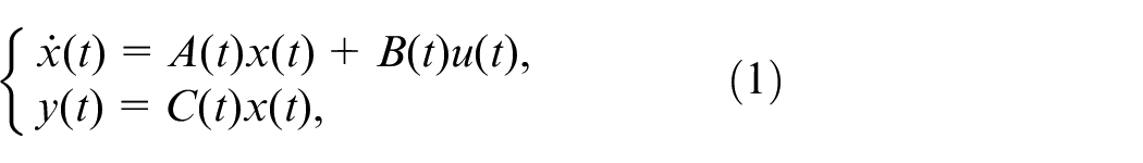
The LTV system can be described as

$$\{\begin{array}{c}\stackrel{·}{x}(t)=A(t)x(t)+B(t)u(t),\hfill \\ \multicolumn{1}{c}{y(t)=C(t)x(t),}\end{array}$$

(1)

where $\stackrel{·}{x}:=\frac{\mathrm{d}x}{\mathrm{d}t}$ , $x(t)$ is the $n\times 1$ state, $y(t)$ is the $m\times 1$ output and $u(t)$ is the $r\times 1$ input, respectively. $A(t)\in \mathbb{P}\mathbb{C}(J,{\mathbb{R}}^{n\times n})\cap {\mathbb{C}}^{n-2}(J,{\mathbb{R}}^{n\times n})$ , $B(t)\in \mathbb{P}\mathbb{C}(J,{\mathbb{R}}^{n\times r})$ and $C(t)\in \mathbb{P}\mathbb{C}(J,{\mathbb{R}}^{m\times n})\cap {\mathbb{C}}^{n-1}(J,{\mathbb{R}}^{m\times n})$ are the coefficient matrices.

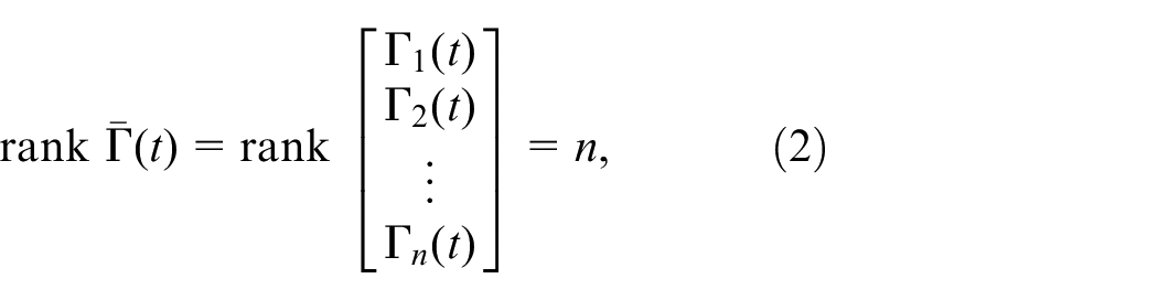
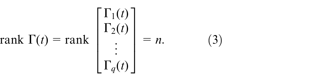
• Lemma 1. Observability Criterion. ³⁸ The matrix pair $\{A(t),C(t)\}$ of LTV system (1) is observable if there is a finite $t\in J$ such that

$$\mathrm{rank}\overline{\mathrm{\Gamma }}(t)=\mathrm{rank}\left[\begin{array}{c}{\mathrm{\Gamma }}_1(t)\hfill \\ \multicolumn{1}{c}{{\mathrm{\Gamma }}_2(t)}\\ \multicolumn{1}{c}{⋮}\\ \multicolumn{1}{c}{{\mathrm{\Gamma }}_n(t)}\end{array}\right]=n,$$

(2)

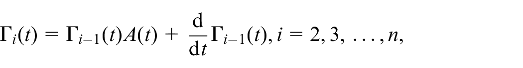
where

$${\mathrm{\Gamma }}_i(t)={\mathrm{\Gamma }}_{i-1}(t)A(t)+\frac{\mathrm{d}}{\mathrm{d}t}{\mathrm{\Gamma }}_{i-1}(t),i=2,3,\dots ,n,$$

with

$${\mathrm{\Gamma }}_1(t)=C(t).$$

Assume that $\{A(t),C(t)\}$ is observable, and define observability index $q$ as the least integer such that equation (2) holds, that is,

$$\mathrm{rank}\mathrm{\Gamma }(t)=\mathrm{rank}\left[\begin{array}{c}{\mathrm{\Gamma }}_1(t)\hfill \\ \multicolumn{1}{c}{{\mathrm{\Gamma }}_2(t)}\\ \multicolumn{1}{c}{⋮}\\ \multicolumn{1}{c}{{\mathrm{\Gamma }}_q(t)}\end{array}\right]=n.$$

(3)

Let $h(t)$ be the $k\times 1$ estimated vector in the following form

$$h(t)=K(t)x(t),$$

(4)

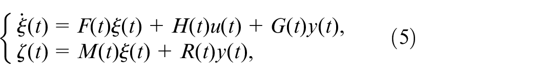
where matrix $K(t)\in \mathbb{P}\mathbb{C}(J,{\mathbb{R}}^{k\times n})$ is given. Following observer system is presented to estimate the estimated vector $h(t)$

$$\{\begin{array}{c}\stackrel{·}{\xi }(t)=F(t)\xi (t)+H(t)u(t)+G(t)y(t),\hfill \\ \multicolumn{1}{c}{\zeta (t)=M(t)\xi (t)+R(t)y(t),}\end{array}$$

(5)

where $\xi (t)$ is the $\mu \times 1$ observer state, $M(t)$ , $H(t)$ , $R(t)$ , $G(t)$ and $F(t)$ are real matrices of proper order.

• Assumption 1. The $\{A(t),C(t)\}$ of LTV system (1) is observable.

• Assumption 2. $C(t)$ and $K(t)$ are row full rank.

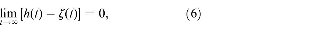
• Problem 1. Given system (1) satisfying Assumptions 1 and 2, find the set of system coefficient matrices $M(t)$ , $H(t)$ , $R(t)$ , $G(t)$ , and $F(t)$ that makes

$$\underset{t\to \infty }{lim}[h(t)-\zeta (t)]=0,$$

(6)

for arbitrarily given $x(0)$ , $\xi (0)$ and $u(t)$ .

Preliminaries

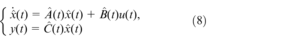
Introduce a time-varying transformation

$$x(t)=S(t)\hat{x}(t),$$

(7)

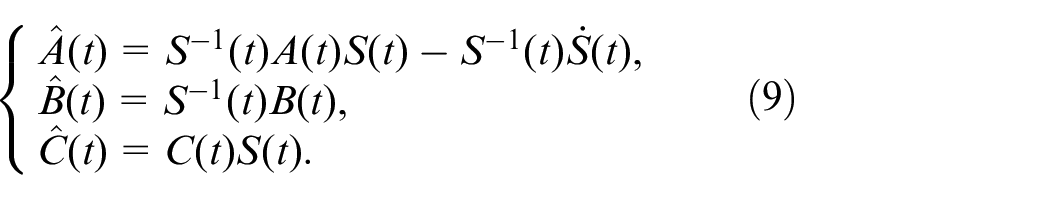
with $S(t)\in \mathbb{P}\mathbb{C}(J,{\mathbb{R}}^{n\times n})\cap {\mathbb{C}}^1(J,{\mathbb{R}}^{n\times n})$ and $S(t)$ , $S^{-1}(t)$ , $\stackrel{·}{S}(t)$ are bounded for $t\in J$ . This transformation transforms system (1) into

$$\{\begin{array}{c}\stackrel{·}{\hat{x}}(t)=\hat{A}(t)\hat{x}(t)+\hat{B}(t)u(t),\hfill \\ \multicolumn{1}{c}{y(t)=\hat{C}(t)\hat{x}(t)}\end{array}$$

(8)

where

$$\{\begin{array}{c}\hat{A}(t)=S^{-1}(t)A(t)S(t)-S^{-1}(t)\stackrel{·}{S}(t),\hfill \\ \multicolumn{1}{c}{\hat{B}(t)=S^{-1}(t)B(t),}\\ \multicolumn{1}{c}{\hat{C}(t)=C(t)S(t).}\end{array}$$

(9)

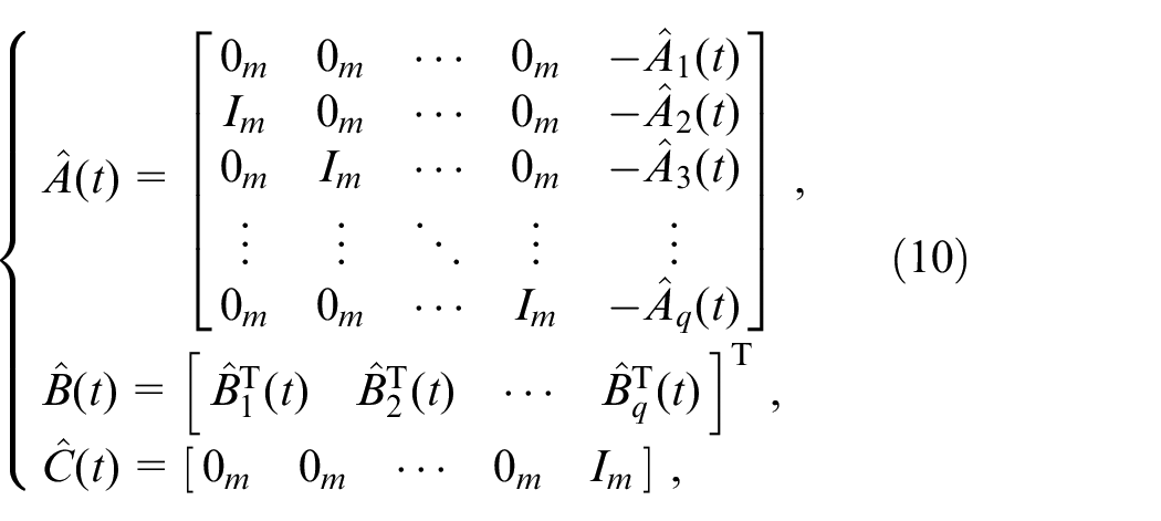
• Lemma 2. Shieh et al. ³⁹ The observable LTV system (1) can be converted to an observable canonical form (8) with the following coefficient matrices

$$\{\begin{array}{c}\hat{A}(t)=\left[\begin{array}{ccccc}{0}_m\hfill & 0_m\hfill & \cdots \hfill & 0_m\hfill & -{\hat{A}}_1(t)\hfill \\ \multicolumn{1}{c}{I_m}& 0_m\hfill & \cdots \hfill & 0_m\hfill & -{\hat{A}}_2(t)\hfill \\ \multicolumn{1}{c}{0_m}& I_m\hfill & \cdots \hfill & 0_m\hfill & -{\hat{A}}_3(t)\hfill \\ \multicolumn{1}{c}{⋮}& ⋮\hfill & \ddots \hfill & ⋮\hfill & ⋮\hfill \\ \multicolumn{1}{c}{0_m}& 0_m\hfill & \cdots \hfill & I_m\hfill & -{\hat{A}}_q(t)\hfill \end{array}\right],\hfill \\ \multicolumn{1}{c}{\hat{B}(t)={\left[\begin{array}{cccc}{\hat{B}}_1^{\mathrm{T}}(t)\hfill & {\hat{B}}_2^{\mathrm{T}}(t)\hfill & \cdots \hfill & {\hat{B}}_q^{\mathrm{T}}(t)\hfill \end{array}\right]}^{\mathrm{T}},}\\ \multicolumn{1}{c}{\hat{C}(t)=\left[\begin{array}{ccccc}{0}_m\hfill & 0_m\hfill & \cdots \hfill & 0_m\hfill & I_m\hfill \end{array}\right],}\end{array}$$

(10)

by the time-varying transformation (7) with

$$S(t)=\left[\begin{array}{cccc}{S}_1(t)\hfill & S_2(t)\hfill & \cdots \hfill & S_q(t)\hfill \end{array}\right],$$

(11)

where

$$\{\begin{array}{c}{S}_1(t)=(\hat{C}(t){\mathrm{\Gamma }}^{-1}(t){)}^{\mathrm{T}},\hfill \\ \multicolumn{1}{c}{S_i(t)=A(t)S_{i-1}(t)-{\stackrel{·}{S}}_{i-1}(t),i=2,\dots ,q,}\end{array}$$

(12)

with $\mathrm{\Gamma }(t)$ in equation (3) and $q$ is observability index.

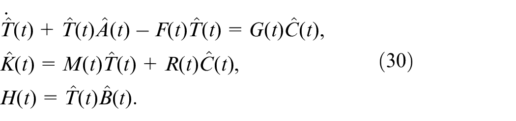
• Lemma 3. Trumpf ⁴⁰ and Rotella and Zambettakis ⁴¹ Assume that the LTV system (1) is observable. For arbitrarily given $x(0)$ , $\xi (0)$ , and $u(t)$ , equation (6) holds if and only if $F(t)$ is a Hurwitz matrix and there is a matrix $T(t)\in \mathbb{P}\mathbb{C}(J,{\mathbb{R}}^{\mu \times n})\cap {\mathbb{C}}^1(J,{\mathbb{R}}^{\mu \times n})$ satisfying

$$\stackrel{·}{T}(t)+T(t)A(t)-G(t)C(t)=F(t)T(t),$$

(13)

$$K(t)-R(t)C(t)=M(t)T(t),$$

(14)

$$H(t)=T(t)B(t).$$

(15)

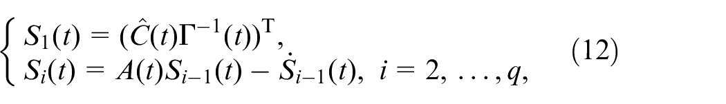
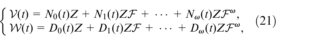
Let us introduce the solution to the first-order homogeneous GSE with time-varying coefficients

$$\mathcal{V}(t)\mathcal{F}=\mathcal{A}(t)\mathcal{V}(t)+\mathcal{B}(t)\mathcal{W}(t),$$

(16)

where $\mathcal{A}(t)\in \mathbb{P}\mathbb{C}(J,{\mathbb{R}}^{n\times q})$ , $\mathcal{B}(t)\in \mathbb{P}\mathbb{C}(J,{\mathbb{R}}^{n\times r})$ , $q+r>n$ , and $\mathcal{F}\in {\mathbb{C}}^{p\times p}$ are coefficient matrices, and $\mathcal{V}(t)\in \mathbb{P}\mathbb{C}(J,{\mathbb{C}}^{q\times p})$ , $\mathcal{W}(t)\in \mathbb{P}\mathbb{C}(J,{\mathbb{C}}^{r\times p})$ are parameter matrices to be solved.

• Definition 1. Duan ³³ The pair $\{\mathrm{sI}-\mathcal{A}(t),\mathcal{B}(t)\}$ are called to be left coprime with rank $\alpha$ over $J$ if the pair $\{\mathrm{sI}-\mathcal{A}(t),\mathcal{B}(t)\}$ are $\mathcal{F}$ -left coprime with rank $\alpha$ for arbitrary $\mathcal{F}\in {\mathbb{C}}^{p\times p}$ , namely,

$$\mathrm{rank}\left[\begin{array}{cc}\mathrm{sI}-\mathcal{A}(t)\hfill & \mathcal{B}(t)\hfill \end{array}\right]=\alpha ,\forall t\in J,s\in \mathrm{eig}(\mathcal{F}).$$

(17)

According to Definition 1, when the rank condition (17) is met, there are unimodular matrices $P(t,s)$ and $Q(t,s)$ satisfying

$$P(t,s)\left[\begin{array}{cc}\mathrm{sI}-\mathcal{A}(t)\hfill & -B(t)\hfill \end{array}\right]Q(t,s)=\left[\begin{array}{cc}\Sigma (t,s)\hfill & 0\hfill \end{array}\right],$$

(18)

where $\Sigma (t,s)\in \mathbb{P}\mathbb{C}(J,{\mathbb{R}}^{n\times n})[s]$ is generally in a diagonal form, meeting

$$\det \Sigma (t,s)\ne 0,\forall t\in J,s\in \mathrm{eig}(\mathcal{F}),$$

and $Q(t,s)$ can be partitioned as

$$Q(t,s)=\left[\begin{array}{cc}*\hfill & N(t,s)\hfill \\ \multicolumn{1}{c}{*}& D(t,s)\hfill \end{array}\right],$$

where $N(t,s)\in \mathbb{P}\mathbb{C}(J,{\mathbb{R}}^{q\times {\beta }_0})$ and $D(t,s)\in \mathbb{P}\mathbb{C}(J,{\mathbb{R}}^{r\times {\beta }_0})$ , ${\beta }_0=q+r-n$ , then equation (18) leads to

$${(\mathrm{sI}-\mathcal{A}(t))}^{-1}\mathcal{B}(t)-N(t,s)D^{-1}(t,s)=0.$$

(19)

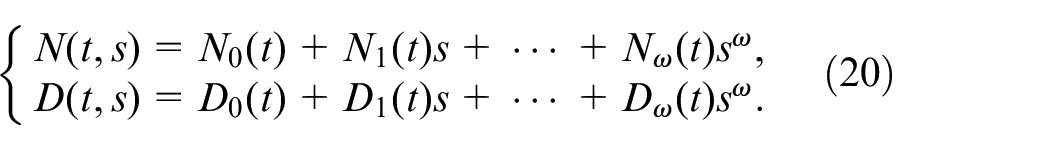
This is well-known right coprime factorization (RCF) of $\{\mathcal{A}(t),\mathcal{B}(t)\}$ . Further, use $\omega$ to denote the maximum degree of $N(t,s)$ and $D(t,s)$ , then we have

$$\{\begin{array}{c}N(t,s)=N_0(t)+N_1(t)s+\cdots +N_{\omega }(t)s^{\omega },\hfill \\ \multicolumn{1}{c}{D(t,s)=D_0(t)+D_1(t)s+\cdots +D_{\omega }(t)s^{\omega }.}\end{array}$$

(20)

To solve the GSE (16), we present following result.

• Theorem 1. Duan ³³ Let $\mathcal{F}\in {\mathbb{C}}^{p\times p}$ , and the pair $\{\mathrm{sI}-\mathcal{A}(t),\mathcal{B}(t)\}$ be $\mathcal{F}$ -left coprime over $J$ . Set $N(t,s)$ and $D(t,s)$ , a pair of right coprime polynomial matrices satisfying (19) and having the form of (20), then for $t\in J$ , a general solution to the GSE (16) is

$$\{\begin{array}{c}\mathcal{V}(t)=N_0(t)Z+N_1(t)Z\mathcal{F}+\cdots +N_{\omega }(t)Z{\mathcal{F}}^{\omega },\hfill \\ \multicolumn{1}{c}{\mathcal{W}(t)=D_0(t)Z+D_1(t)Z\mathcal{F}+\cdots +D_{\omega }(t)Z{\mathcal{F}}^{\omega },}\end{array}$$

(21)

with $Z\in {\mathbb{C}}^{{\beta }_0\times p}$ an arbitrary parameter matrix.

Main results

It is well-known that the full-order observer possesses a certain degree of redundancy. Instead of having to recreate a full-dimensional observer, the output variables can provide $m$ state variables. Therefore, according to Lemma 2, we introduce the time-varying transformation (7), convert system (1) into the partition form (8) with coefficients

$$\{\begin{array}{c}\hat{A}(t)=\left[\begin{array}{cc}{\hat{A}}_{11}(t)\hfill & {\hat{A}}_{12}(t)\hfill \\ \multicolumn{1}{c}{{\hat{A}}_{21}(t)}& {\hat{A}}_{22}(t)\hfill \end{array}\right],\hat{B}(t)=\left[\begin{array}{c}{\hat{B}}_1(t)\hfill \\ \multicolumn{1}{c}{{\hat{B}}_2(t)}\end{array}\right],\hfill \\ \multicolumn{1}{c}{\hat{C}(t)=\left[\begin{array}{cc}{\hat{C}}_1\hfill & {\hat{C}}_2\hfill \end{array}\right]=\left[\begin{array}{cc}{0}_{m\times (n-m)}\hfill & I_m\hfill \end{array}\right]}\end{array}$$

(22)

where ${\hat{A}}_{11}(t)\in \mathbb{P}\mathbb{C}(J,{\mathbb{R}}^{(n-m)\times (n-m)})\cap {\mathbb{C}}^{n-2}(J,{\mathbb{R}}^{(n-m)\times (n-m)})$ , ${\hat{A}}_{12}(t)\in \mathbb{P}\mathbb{C}(J,{\mathbb{R}}^{(n-m)\times m})\cap {\mathbb{C}}^{n-2}(J,{\mathbb{R}}^{(n-m)\times m})$ , ${\hat{A}}_{21}(t)\in \mathbb{P}\mathbb{C}(J,{\mathbb{R}}^{m\times (n-m)})\cap {\mathbb{C}}^{n-2}(J,{\mathbb{R}}^{m\times (n-m)})$ , ${\hat{A}}_{22}(t)\in \mathbb{P}\mathbb{C}(J,{\mathbb{R}}^{m\times m})\cap {\mathbb{C}}^{n-2}(J,{\mathbb{R}}^{m\times m})$ , ${\hat{B}}_1(t)\in \mathbb{P}\mathbb{C}(J,{\mathbb{R}}^{(n-m)\times r})$ , ${\hat{B}}_2(t)\in \mathbb{P}\mathbb{C}(J,{\mathbb{R}}^{m\times r})$ , ${\hat{C}}_1\in {\mathbb{R}}^{m\times (n-m)}$ , ${\hat{C}}_2\in {\mathbb{R}}^{m\times m}$ . 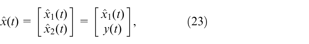The new state $\hat{x}(t)$ can be divided into

$$\hat{x}(t)=\left[\begin{array}{c}{\hat{x}}_1(t)\hfill \\ \multicolumn{1}{c}{{\hat{x}}_2(t)}\end{array}\right]=\left[\begin{array}{c}{\hat{x}}_1(t)\hfill \\ \multicolumn{1}{c}{y(t)}\end{array}\right],$$

(23)

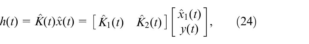
with the $(n-m)$ -dimensional ${\hat{x}}_1(t)$ and $m$ -dimensional output $y(t)$ . This implies that ${\hat{x}}_2(t)$ can be obtained directly without reconstruction. We only need to design the $(n-m)$ -dimensional ROFO for the LTV system (1). Furthermore, the estimated vector (4) also can be partitioned into the following form

$$h(t)=\hat{K}(t)\hat{x}(t)=\left[\begin{array}{cc}{\hat{K}}_1(t)\hfill & {\hat{K}}_2(t)\hfill \end{array}\right]\left[\begin{array}{c}{\hat{x}}_1(t)\hfill \\ \multicolumn{1}{c}{y(t)}\end{array}\right],$$

(24)

where $\hat{K}(t)=K(t)S(t)$ , ${\hat{K}}_1(t)\in \mathbb{P}\mathbb{C}(J,{\mathbb{R}}^{k\times (n-m)})$ , and ${\hat{K}}_2(t)\in \mathbb{P}\mathbb{C}(J,{\mathbb{R}}^{k\times m})$ .

• Remark 1. Observing the scalar linear functional of states may be much simpler than that of the whole. Therefore, Luenberger ⁴² firstly proposed a primary result, the upper bound on the order of scalar functional observer is $q-1$ . Correspondingly, when the linear function to be estimated has the dimension of $k$ , the order of the multi-functional observer is $\mu =({\mu }_1+\cdots +{\mu }_k)$ , and as a result of the above discussion, it will be less than $k(q-1)$ , where ${\mu }_i$ represents order of the $i$ -th scalar FO. It is also noted that for any fully observable system, there is $q-1\le n-m$ holds, and in most cases $q-1$ is much smaller than $n-m$ , then $k(q-1)\le (n-m)$ is possible, otherwise, $\mu =(n-m)$ will be the order of the minimum-order observer. In other words, the upper bound of the order of multi-functional observer is equal to the smaller of $k(q-1)$ and $(n-m)$ , but in either case, it will constitute a ROFO of LTV system (1) and have the unified form as shown in (5).

Existence conditions for ROFO system

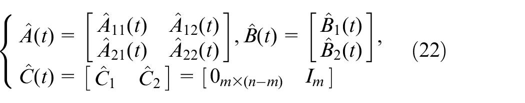
For the transformed system (22), sufficient conditions for the existence of ROFO can be deduced in the following theorem with block forms.

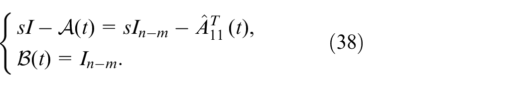
• Theorem 2. Assume that system (1) satisfy Assumptions 1 and 2. Then, the system (5) is a ROFO with $\mu$ -order for the transformed system (22) if $F(t)$ is a Hurwitz matrix, and there exits a block matrix $\hat{T}(t)=\left[\begin{array}{cc}{\hat{T}}_1(t)\hfill & {\hat{T}}_2(t)\hfill \end{array}\right]$ with ${\hat{T}}_1(t)\in {\mathbb{C}}^1(J,{\mathbb{R}}^{\mu \times (n-m)})$ and ${\hat{T}}_2(t)\in {\mathbb{C}}^1(J,{\mathbb{R}}^{\mu \times m})$ satisfying

$${\hat{T}}_1(t){\hat{A}}_{12}(t)+{\hat{T}}_2(t){\hat{A}}_{22}(t)+{\stackrel{·}{\hat{T}}}_2(t)-F(t){\hat{T}}_2(t)=G(t),$$

(25)

$${\hat{T}}_1(t){\hat{A}}_{11}(t)+{\hat{T}}_2(t){\hat{A}}_{21}(t)+{\stackrel{·}{\hat{T}}}_1(t)-F(t){\hat{T}}_1(t)=0,$$

(26)

and

$$H(t)={\hat{T}}_1(t){\hat{B}}_1(t)+{\hat{T}}_2(t){\hat{B}}_2(t),$$

(27)

$${\hat{K}}_2(t)=M(t){\hat{T}}_2(t)+R(t),$$

(28)

$${\hat{K}}_1(t)=M(t){\hat{T}}_1(t).$$

(29)

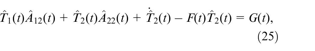
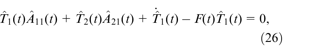
Proof. By deducing Lemma 3, the observer (5) of system (22) exists when the following conditions are met

$$\begin{array}{c}\stackrel{·}{\hat{T}}(t)+\hat{T}(t)\hat{A}(t)-F(t)\hat{T}(t)=G(t)\hat{C}(t),\hfill \\ \hat{K}(t)=M(t)\hat{T}(t)+R(t)\hat{C}(t),\hfill \\ H(t)=\hat{T}(t)\hat{B}(t).\hfill \end{array}$$

(30)

Then substitute corresponding matrices with the ones defined in system (22), and we can get equations (25)–(29). The proof is completed.

Parametric form of observer gain

Based on Theorem 2, we propose existence conditions of ROFO for LTV systems. In this subsection, completely parameterized expressions of the gain matrices of the ROFO are established by using the parametric solutions of the GSE proposed above, and the following theorem is given.

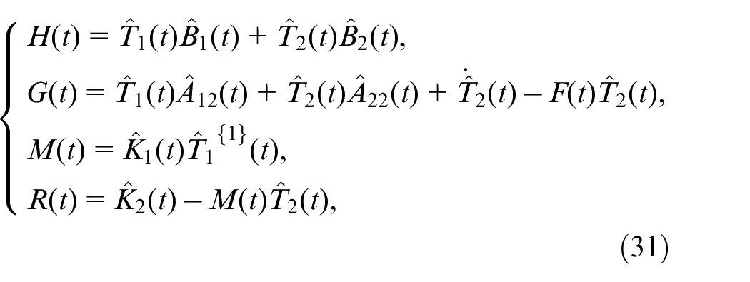
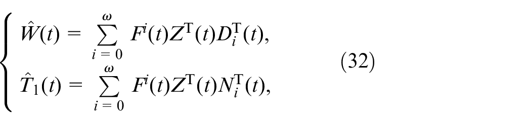
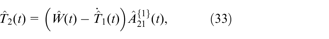
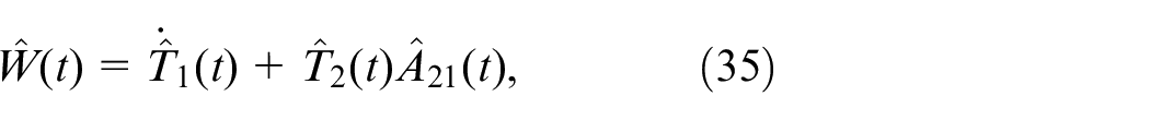
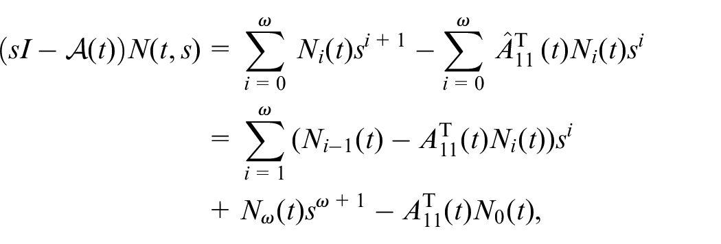
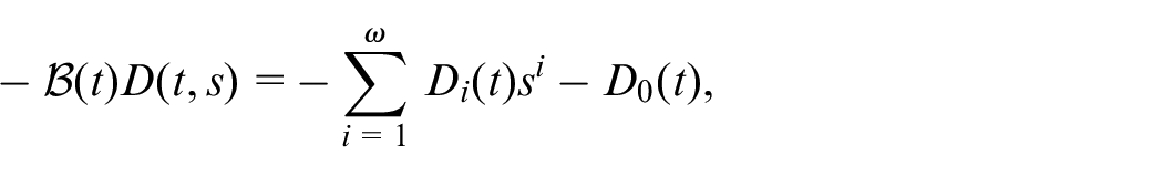
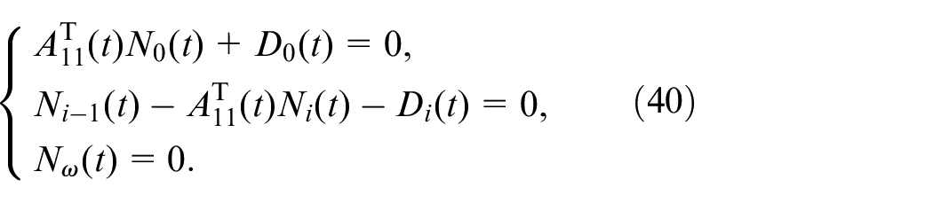
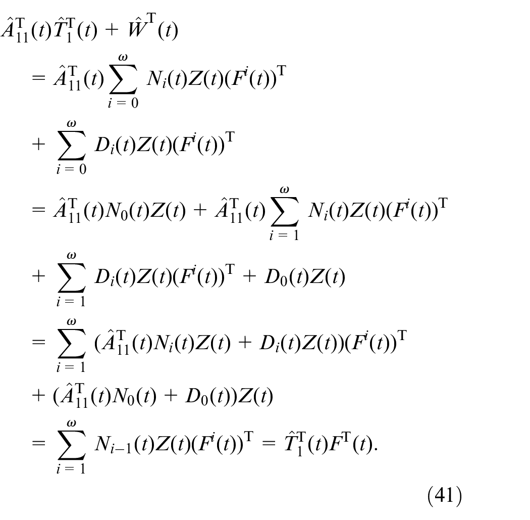
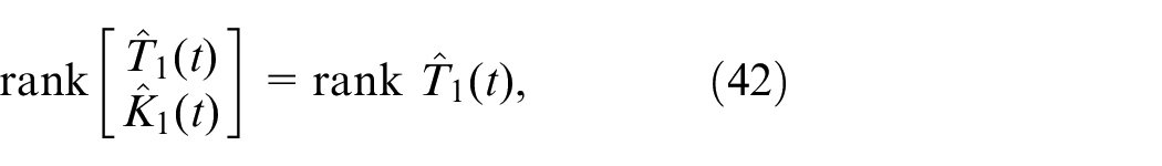
• Theorem 3. Assume that system (1) satisfy Assumptions 1 and 2, $F(t)\in {\mathbb{R}}^{\mu \times \mu }$ is an arbitrary Hurwitz matrix. Further, preset right coprime matrices $D(t,s)$ and $N(t,s)$ in the form of (20) and satisfying (19), with $\mathcal{A}(t)={\hat{A}}_{11}^{\mathrm{T}}(t)$ , $\mathcal{B}(t)=I_{n-m}$ . Then, coefficient matrices of the ROFO (5) with $\mu$ -order can be parametrized as

$$\{\begin{array}{c}H(t)={\hat{T}}_1(t){\hat{B}}_1(t)+{\hat{T}}_2(t){\hat{B}}_2(t),\hfill \\ G(t)={\hat{T}}_1(t){\hat{A}}_{12}(t)+{\hat{T}}_2(t){\hat{A}}_{22}(t)+{\stackrel{·}{\hat{T}}}_2(t)-F(t){\hat{T}}_2(t),\hfill \\ M(t)={\hat{K}}_1(t){{\hat{T}}_1}^{\left\{1\right\}}(t),\hfill \\ R(t)={\hat{K}}_2(t)-M(t){\hat{T}}_2(t),\hfill \end{array}$$

(31)

with

$$\{\begin{array}{c}\hat{W}(t)=\sum _{i=0}^{\omega }{F}^i(t)Z^{\mathrm{T}}(t)D_i^{\mathrm{T}}(t),\hfill \\ \multicolumn{1}{c}{{\hat{T}}_1(t)=\sum _{i=0}^{\omega }{F}^i(t)Z^{\mathrm{T}}(t)N_i^{\mathrm{T}}(t),}\end{array}$$

(32)

and

$${\hat{T}}_2(t)=(\hat{W}(t)-{\stackrel{·}{\hat{T}}}_1(t)){\hat{A}}_{21}^{\left\{1\right\}}(t),$$

(33)

if there is an arbitrary matrix $Z(t)\in \mathbb{P}\mathbb{C}(J,{\mathbb{R}}^{(n-m)\times \mu })$ satisfying

$$\mathrm{rank}\left[\begin{array}{c}{\hat{T}}_1(t)\hfill \\ \multicolumn{1}{c}{{\hat{K}}_1(t)}\end{array}\right]=\mathrm{rank}{\hat{T}}_1(t),$$

(34)

and $[•{]}^{\left\{1\right\}}$ denotes the generalized inverse of [•].

Proof. Denote

$$\hat{W}(t)={\stackrel{·}{\hat{T}}}_1(t)+{\hat{T}}_2(t){\hat{A}}_{21}(t),$$

(35)

then equation (26) yields

$${\hat{T}}_1(t){\hat{A}}_{11}(t)+\hat{W}(t)=F(t){\hat{T}}_1(t).$$

(36)

Taking a transpose of equation (36), then we have the following GSE form

$${\hat{T}}_1^{\mathrm{T}}(t)F^{\mathrm{T}}(t)={\hat{A}}_{11}^{\mathrm{T}}(t){\hat{T}}_1^{\mathrm{T}}(t)+{\hat{W}}^{\mathrm{T}}(t),$$

(37)

and corresponding polynomials in equation (19) are

$$\{\begin{array}{c}\mathrm{sI}-\mathcal{A}(t)=s{I}_{n-m}-{\hat{A}}_{11}^T(t),\hfill \\ \mathcal{B}(t)=I_{n-m}.\hfill \end{array}$$

(38)

Equation (19) can be written as

$$(\mathrm{sI}-\mathcal{A}(t))N(t,s)-\mathcal{B}(t)D(t,s)=0,$$

(39)

then using (20) and (38), we have

$$\begin{array}{c}\multicolumn{1}{c}{(\mathrm{sI}-\mathcal{A}(t))N(t,s)=\sum _{i=0}^{\omega }{N}_i(t)s^{i+1}-\sum _{i=0}^{\omega }{\hat{A}}_{11}^{\mathrm{T}}(t)N_i(t)s^i}\\ =\sum _{i=1}^{\omega }(N_{i-1}(t)-A_{11}^{\mathrm{T}}(t)N_i(t))s^i\hfill \\ +N_{\omega }(t)s^{\omega +1}-A_{11}^{\mathrm{T}}(t)N_0(t),\hfill \end{array}$$

and

$$-\mathcal{B}(t)D(t,s)=-\sum _{i=1}^{\omega }{D}_i(t)s^i-D_0(t),$$

substituting the above two relations into (39) to get

$$\{\begin{array}{c}{A}_{11}^{\mathrm{T}}(t)N_0(t)+D_0(t)=0,\hfill \\ N_{i-1}(t)-A_{11}^{\mathrm{T}}(t)N_i(t)-D_i(t)=0,\hfill \\ N_{\omega }(t)=0.\hfill \end{array}$$

(40)

Using the expressions in (32) and (37), we obtain

$$\begin{array}{c}{\hat{A}}_{11}^{\mathrm{T}}(t){\hat{T}}_1^{\mathrm{T}}(t)+{\hat{W}}^{\mathrm{T}}(t)\hfill \\ ={\hat{A}}_{11}^{\mathrm{T}}(t)\sum _{i=0}^{\omega }{N}_i(t)Z(t)(F^i(t){)}^{\mathrm{T}}\hfill \\ +\sum _{i=0}^{\omega }{D}_i(t)Z(t)(F^i(t){)}^{\mathrm{T}}\hfill \\ ={\hat{A}}_{11}^{\mathrm{T}}(t)N_0(t)Z(t)+{\hat{A}}_{11}^{\mathrm{T}}(t)\sum _{i=1}^{\omega }{N}_i(t)Z(t)(F^i(t){)}^{\mathrm{T}}\hfill \\ +\sum _{i=1}^{\omega }{D}_i(t)Z(t)(F^i(t){)}^{\mathrm{T}}+D_0(t)Z(t)\hfill \\ =\sum _{i=1}^{\omega }({\hat{A}}_{11}^{\mathrm{T}}(t)N_i(t)Z(t)+D_i(t)Z(t))(F^i(t){)}^{\mathrm{T}}\hfill \\ +({\hat{A}}_{11}^{\mathrm{T}}(t)N_0(t)+D_0(t))Z(t)\hfill \\ =\sum _{i=1}^{\omega }{N}_{i-1}(t)Z(t)(F^i(t){)}^{\mathrm{T}}={\hat{T}}_1^{\mathrm{T}}(t)F^{\mathrm{T}}(t).\hfill \end{array}$$

(41)

This indicates that the parametric solutions of ${\hat{T}}_1(t)$ and $\hat{W}(t)$ represented by (32) satisfying (37). Then, equation (33) indicates (35). Combining equations (25)–(29) yields (31). Particular, the matrix $M(t)$ is determined by (29), and it is solvable if and only if

$$\mathrm{rank}\left[\begin{array}{c}{\hat{T}}_1(t)\hfill \\ \multicolumn{1}{c}{{\hat{K}}_1(t)}\end{array}\right]=\mathrm{rank}{\hat{T}}_1(t),$$

(42)

which can be guaranteed by the free parameter $Z(t)$ . This completes the proof.

• Remark 2. In the framework of LTV systems, Theorem 3 gives all the observer gains that meet the most basic requirements, where there exists the free parameter $Z(t)$ , and because of its existence, the above condition (42) is easily satisfied.

• Remark 3. It is easy to infer that the performance of the observer is determined by the matrices $F(t)$ and $M(t)$ , and the Hurwitz matrix $F(t)$ can be arbitrarily selected from Theorem 3 to determine the observer error system. In the design process, if the degrees of freedom still exist, the matrix $M(t)$ can be designed to determine the observer.

• Remark 4. Although there are many matrices involved in the design process, the only ones that can be selected arbitrarily are the Hurwitz matrix $F(t)$ and the parameter matrix $Z(t)$ that makes (42) true. Once these two matrices are determined, others can be represented by related parameters to construct the observer.

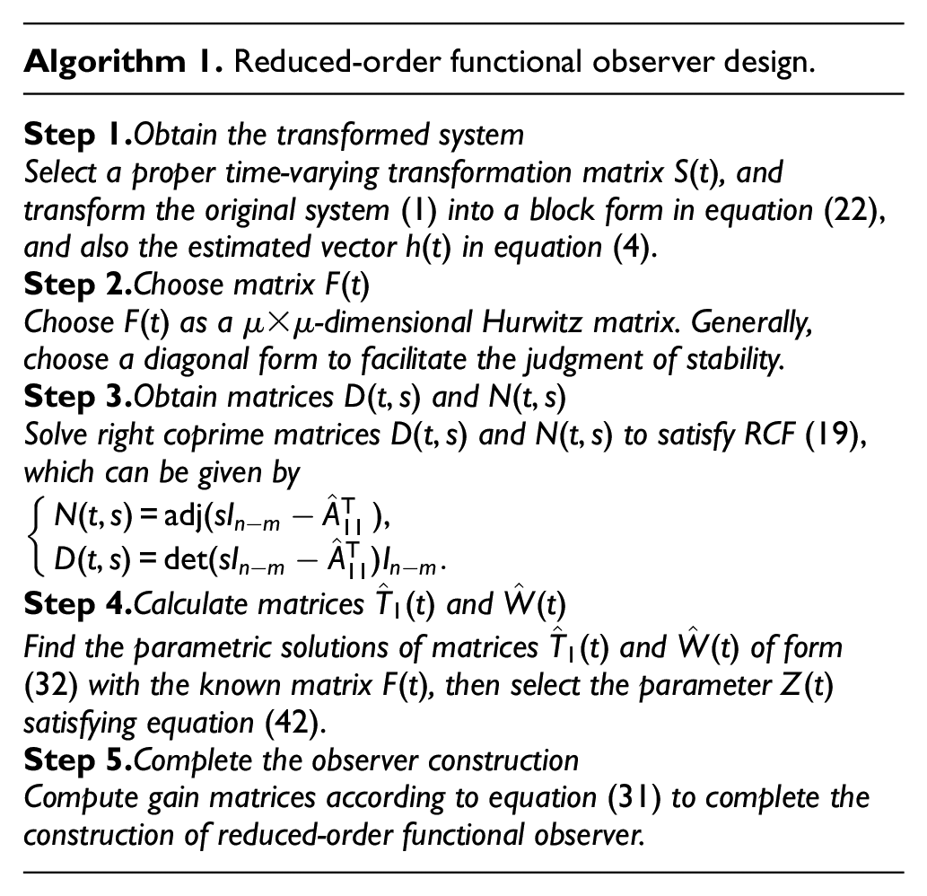
Design algorithm

Based on the above derivation, we propose the following algorithm for parameterized design of a ROFO of LTV system (1) in the form of system (5).

• Remark 5. By selecting the matrix $F(t)$ , the convergence rate of the observation error can be controlled, so that the error dynamic system can be transformed into a linear one with the desired characteristic structure.

• Remark 6. The main advantages of the proposed approach are all degrees of freedom are provided by $Z(t)$ . When $Z(t)$ satisfying the condition (34) does not exist, we can add the order of observer to offer more sufficient degrees of freedom to ensure the existence of the solution.

Algorithm 1. Reduced-order functional observer design.

Step 1. Obtain the transformed system Select a proper time-varying transformation matrix $S(t)$ , and transform the original system (1) into a block form in equation (22), and also the estimated vector $h(t)$ in equation (4).Step 2.Choose matrix $F(t)$ Choose $F(t)$ as a $\mu \times \mu$ -dimensional Hurwitz matrix. Generally, choose a diagonal form to facilitate the judgment of stability.Step 3.Obtain matrices $D(t,s)$ and $N(t,s)$ Solve right coprime matrices $D(t,s)$ and $N(t,s)$ to satisfy RCF (19), which can be given by $\{\begin{array}{c}N(t,s)=\mathrm{adj}(s{I}_{n-m}-{\hat{A}}_{11}^{\mathrm{T}}),\hfill \\ \multicolumn{1}{c}{D(t,s)=\det (s{I}_{n-m}-{\hat{A}}_{11}^{\mathrm{T}})I_{n-m}.}\end{array}$ Step 4.Calculate matrices ${\hat{T}}_1(t)$ and $\hat{W}(t)$ Find the parametric solutions of matrices ${\hat{T}}_1(t)$ and $\hat{W}(t)$ of form (32) with the known matrix $F(t)$ , then select the parameter $Z(t)$ satisfying equation (42).Step 5.Complete the observer constructionCompute gain matrices according to equation (31) to complete the construction of reduced-order functional observer.

Examples

Numerical simulation

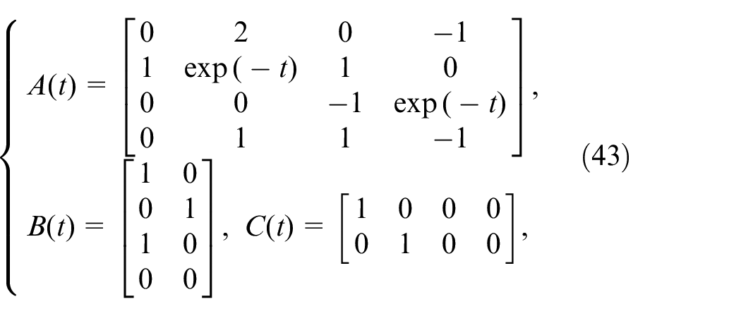
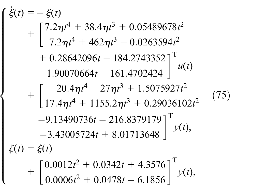
Consider the following 4th-order observable LTV system

$$\{\begin{array}{c}A(t)=\left[\begin{array}{cccc}0\hfill & 2\hfill & 0\hfill & -1\hfill \\ \multicolumn{1}{c}{1}& \exp (-t)\hfill & 1\hfill & 0\hfill \\ \multicolumn{1}{c}{0}& 0\hfill & -1\hfill & \exp (-t)\hfill \\ \multicolumn{1}{c}{0}& 1\hfill & 1\hfill & -1\hfill \end{array}\right],\hfill \\ \multicolumn{1}{c}{B(t)=\left[\begin{array}{cc}1\hfill & 0\hfill \\ \multicolumn{1}{c}{0}& 1\hfill \\ \multicolumn{1}{c}{1}& 0\hfill \\ \multicolumn{1}{c}{0}& 0\hfill \end{array}\right],C(t)=\left[\begin{array}{cccc}1\hfill & 0\hfill & 0\hfill & 0\hfill \\ \multicolumn{1}{c}{0}& 1\hfill & 0\hfill & 0\hfill \end{array}\right],}\end{array}$$

(43)

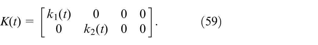
and we will design the ROFO which can asymptotically tracks the functional signal (4) with

$$K(t)=\left[\begin{array}{cccc}0\hfill & 2\cos t\hfill & 1\hfill & 1\hfill \end{array}\right].$$

(44)

According to Lemma 2, the transformation matrix $S(t)$ can be selected as

$$S(t)=\left[\begin{array}{cccc}0\hfill & 0\hfill & 1\hfill & 0\hfill \\ \multicolumn{1}{c}{0}& 0\hfill & 0\hfill & 1\hfill \\ \multicolumn{1}{c}{0}& 1\hfill & \exp (-t)\hfill & -1\hfill \\ \multicolumn{1}{c}{1}& 0\hfill & -1\hfill & 1\hfill \end{array}\right],$$

(45)

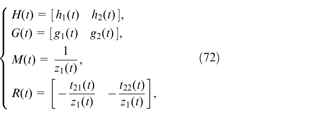
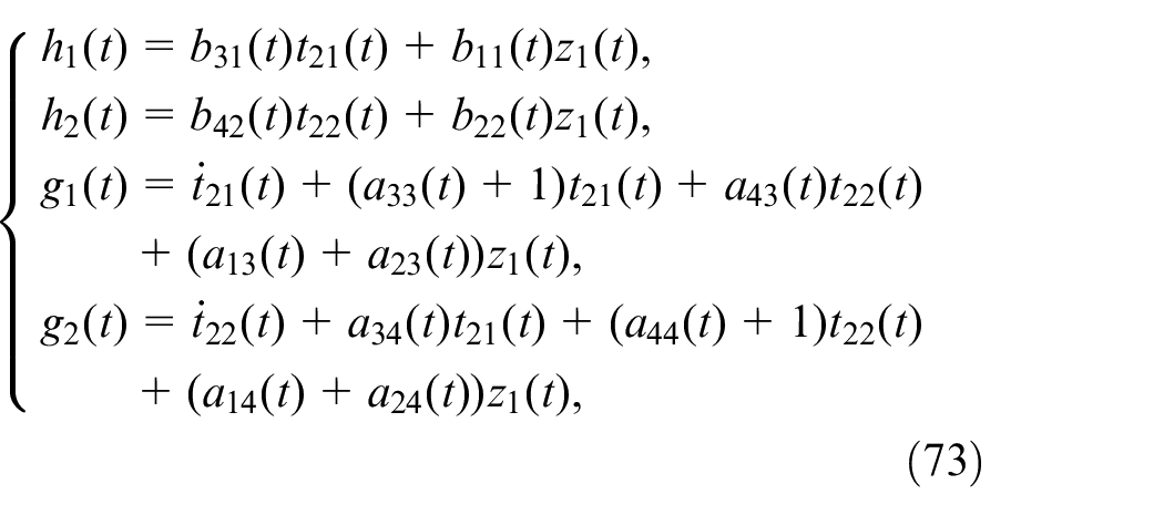
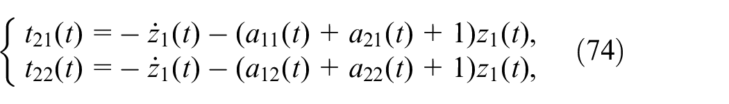
then we can obtain the block transformed system as

$$\{\begin{array}{c}\stackrel{·}{\hat{x}}(t)=\left[\begin{array}{cccc}0\hfill & 0\hfill & -1\hfill & -\exp (-t)-1\hfill \\ \multicolumn{1}{c}{0}& 0\hfill & \exp (-t)+1\hfill & 3\exp (-t)\hfill \\ \multicolumn{1}{c}{1}& 0\hfill & -1\hfill & -1\hfill \\ \multicolumn{1}{c}{0}& 1\hfill & \exp (-t)+1\hfill & \exp (-t)-1\hfill \end{array}\right]\hat{x}(t)\hfill \\ \multicolumn{1}{c}{+\left[\begin{array}{cc}1\hfill & -1\hfill \\ \multicolumn{1}{c}{1-\exp (-t)}& 1\hfill \\ \multicolumn{1}{c}{1}& 0\hfill \\ \multicolumn{1}{c}{0}& 1\hfill \end{array}\right]u(t),}\\ \multicolumn{1}{c}{y(t)=\left[\begin{array}{cccc}0\hfill & 0\hfill & 1\hfill & 0\hfill \\ \multicolumn{1}{c}{0}& 0\hfill & 0\hfill & 1\hfill \end{array}\right]\hat{x}(t),}\end{array}$$

(46)

and also the functional

$$\begin{array}{c}\hat{K}(t)=\left[\begin{array}{cc}{\hat{K}}_1(t)\hfill & {\hat{K}}_2(t)\hfill \end{array}\right]\hfill \\ =\left[\begin{array}{cccc}1\hfill & 1\hfill & \exp (-t)-1\hfill & 2\cos t\hfill \end{array}\right].\hfill \end{array}$$

(47)

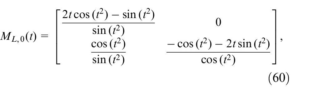
Further, matrices $N(t,s)$ and $D(t,s)$ satisfying (19) can be obtained as

$$\{\begin{array}{c}N(t,s)=\left[\begin{array}{cc}1\hfill & 0\hfill \\ \multicolumn{1}{c}{0}& 1\hfill \end{array}\right],\hfill \\ \multicolumn{1}{c}{D(t,s)=\left[\begin{array}{cc}s\hfill & 0\hfill \\ \multicolumn{1}{c}{0}& s\hfill \end{array}\right].}\end{array}$$

(48)

Choose the Hurwitz matrix $F(t)=-1$ , denote $M(t)=m(t)$ and

$$Z^{\mathrm{T}}(t)=\left[\begin{array}{cc}{z}_1(t)\hfill & z_2(t)\hfill \end{array}\right].$$

(49)

Then, we have matrices ${\hat{T}}_1(t)$ , $\hat{W}(t)$ , and ${\hat{T}}_2(t)$ according to equations (32) and (33)

$$\{\begin{array}{c}{\hat{T}}_1(t)=\left[\begin{array}{cc}{z}_1(t)\hfill & z_2(t)\hfill \end{array}\right],\hfill \\ \multicolumn{1}{c}{\hat{W}(t)=\left[\begin{array}{cc}-z_1(t)\hfill & -z_2(t)\hfill \end{array}\right],}\end{array}$$

(50)

and

$${\hat{T}}_2(t)=\left[\begin{array}{cc}{t}_{21}(t)\hfill & t_{22}(t)\hfill \end{array}\right],$$

(51)

where

$$\{\begin{array}{c}{t}_{21}(t)=-{\stackrel{·}{z}}_1(t)-z_1(t),\hfill \\ \multicolumn{1}{c}{t_{22}(t)=-{\stackrel{·}{z}}_2(t)-z_2(t).}\end{array}$$

(52)

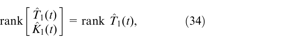
Further, the rank condition (34) should be satisfied, that is, the following equation holds

$$\{\begin{array}{c}m(t)z_1(t)=1,\hfill \\ \multicolumn{1}{c}{m(t)z_2(t)=1,}\end{array}$$

(53)

which indicates $z_1(t)=z_2(t)$ , $m(t)=\frac{1}{z_1(t)}$ .

Substituting the above formula into equation (31), yields the following parametric forms of the ROFO as

$$\{\begin{array}{c}H(t)=\left[\begin{array}{cc}{t}_{21}(t)+(2-\exp (-t))z_1(t)\hfill & t_{21}(t)\hfill \end{array}\right],\hfill \\ G(t)=\left[\begin{array}{cc}{g}_1(t)\hfill & g_2(t)\hfill \end{array}\right],\hfill \\ M(t)=\frac{1}{z_1(t)},\hfill \\ R(t)=\left[\begin{array}{cc}\exp (-t)-1-\frac{t_{21}(t)}{z_1(t)}\hfill & 2\cos t-\frac{t_{21}(t)}{z_1(t)}\hfill \end{array}\right],\hfill \end{array}$$

(54)

with

$$\{\begin{array}{c}{g}_1(t)={\stackrel{·}{t}}_{21}(t)+(\exp (-t)+1)t_{21}(t)+\exp (-t)z_1(t),\hfill \\ \multicolumn{1}{c}{g_2(t)}\\ \multicolumn{1}{c}{={\stackrel{·}{t}}_{21}(t)+(\exp (-t)-1)t_{21}(t)+(2\exp (-t)-1)z_1(t),}\end{array}$$

(55)

and

$$t_{21}(t)=t_{22}(t)=-{\stackrel{·}{z}}_1(t)-z_1(t),$$

(56)

with parameter $z_1(t)=z_2(t)$ are selected arbitrarily.

Consider the initial values as $x_1(0)=x_2(0)=x_3(0)=1$ , $x_4(0)=-1$ , $\xi (0)=0$ , and the control input as $u_1(t)=\sin t$ , $u_2(t)=-3\sin t$ , 0 ≤ t ≤ 30. Meanwhile, without loss of generality, choose $z_1(t)=1$ to have the observer as shown below

$$\{\begin{array}{c}\stackrel{·}{\xi }(t)=-\xi (t)+\left[\begin{array}{cc}1-\exp (-t)\hfill & -1\hfill \end{array}\right]u(t)\hfill \\ \multicolumn{1}{c}{+\left[\begin{array}{cc}-1\hfill & \exp (-t)\hfill \end{array}\right]y(t),}\\ \multicolumn{1}{c}{\zeta (t)=\xi (t)+\left[\begin{array}{cc}\exp (-t)\hfill & 2\cos t+1\hfill \end{array}\right]y(t),}\end{array}$$

(57)

and the simulation results are shown in Figures 1 and 2.

Figure 1.

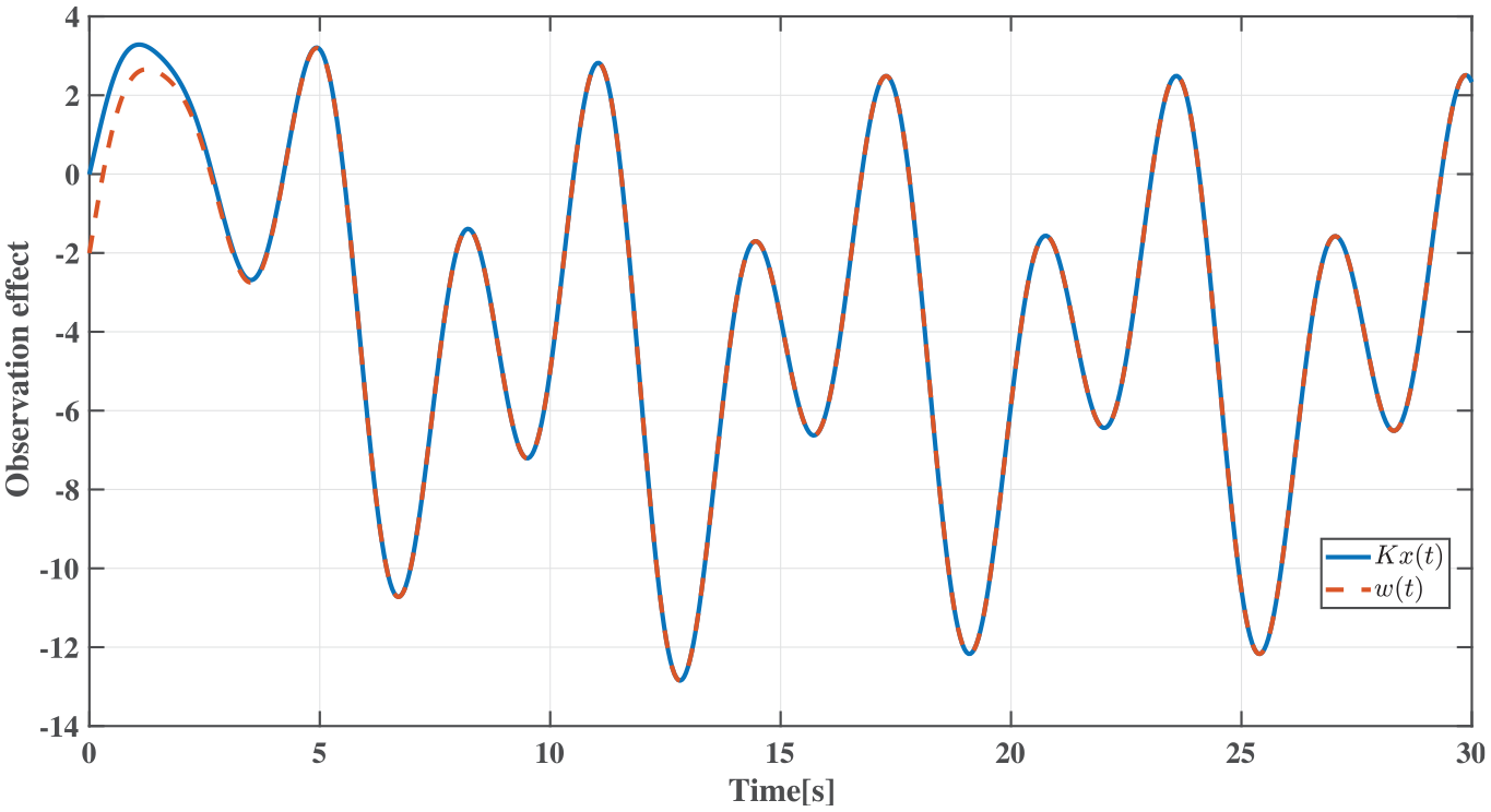
Observation effect of the designed observer.

Figure 2.

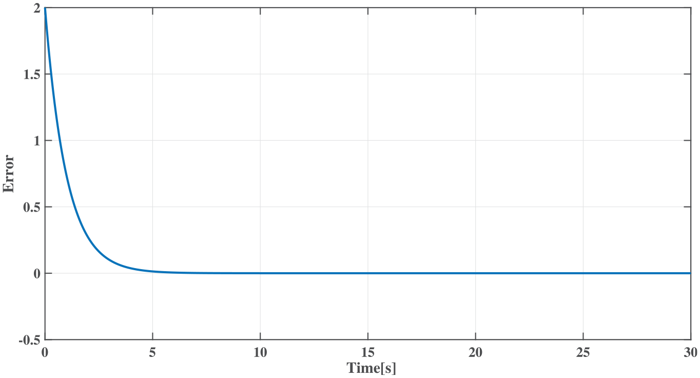
Estimated error.

Figure 1 shows the functional signal to be observed and the output of the designed observer, while Figure 2 shows the observed error defined as $e(t)=h(t)-\zeta (t)$ . From above figures, we can see that the designed observer achieves signal tracking in a short time, which verifies the effectiveness of the proposed method in this paper.

Comparative simulation

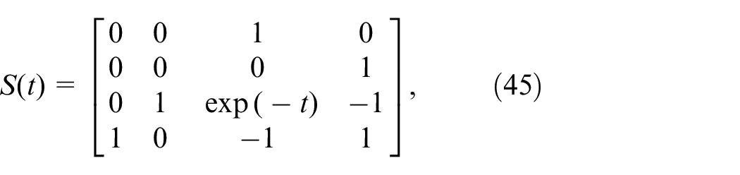
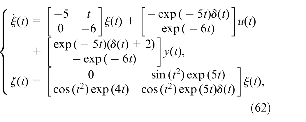
Let us consider the system described in Rotella and Zambettakis ⁴¹ with

$\{\begin{array}{c}A(t)=\left[\begin{array}{cccc}0\hfill & 0\hfill & 0\hfill & -a_1(t)\hfill \\ \multicolumn{1}{c}{1}& 0\hfill & 0\hfill & -a_2(t)\hfill \\ \multicolumn{1}{c}{0}& 1\hfill & 0\hfill & -a_3(t)\hfill \\ \multicolumn{1}{c}{0}& 0\hfill & 1\hfill & -a_4(t)\hfill \end{array}\right],\hfill \\ \multicolumn{1}{c}{B(t)=\left[\begin{array}{c}{b}_1(t)\hfill \\ \multicolumn{1}{c}{b_2(t)}\\ \multicolumn{1}{c}{b_3(t)}\\ \multicolumn{1}{c}{b_4(t)}\end{array}\right],C(t)=\left[\begin{array}{cccc}0\hfill & 0\hfill & 0\hfill & 1\hfill \end{array}\right],}\end{array}$

and the estimated vector (4) are defined by

$$K(t)=\left[\begin{array}{cccc}{k}_1(t)\hfill & 0\hfill & 0\hfill & 0\hfill \\ \multicolumn{1}{c}{0}& k_2(t)\hfill & 0\hfill & 0\hfill \end{array}\right].$$

(59)

In particular, when $k_1(t)=\exp (-t)\sin (t^2)$ and $k_2(t)=\exp (-t)\cos (t^2)$ , using the method in Rotella and Zambettakis ⁴¹ we have

$$M_{L,0}(t)=\left[\begin{array}{cc}\frac{2t\cos (t^2)-\sin (t^2)}{\sin (t^2)}\hfill & 0\hfill \\ \multicolumn{1}{c}{\frac{\cos (t^2)}{\sin (t^2)}}& \frac{-\cos (t^2)-2t\sin (t^2)}{\cos (t^2)}\hfill \end{array}\right],$$

(60)

it is easy to get that system $\stackrel{·}{z}(t)=M_{L,0}(t)z(t)$ is not satisfied with uniform asymptotic stability, which means that the method in Rotella and Zambettakis ⁴¹ is invalid at this time, directly illustrates the effectiveness of this proposed method.

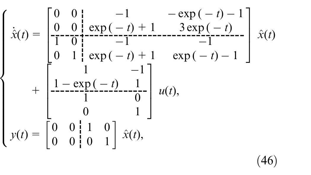
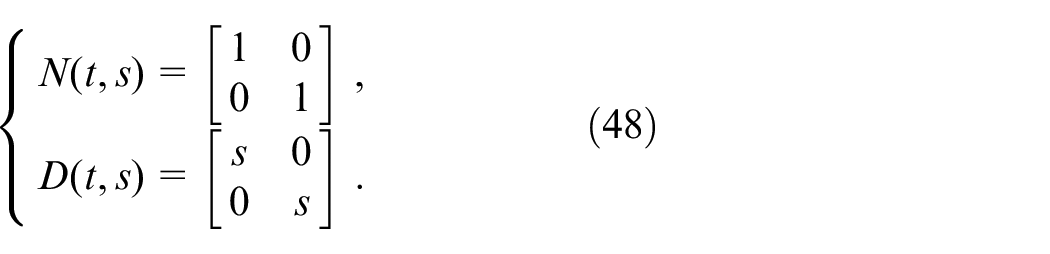
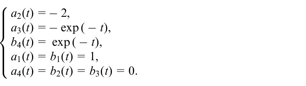
The coefficient matrix $C(t)$ is drawn in the desired form, so the system does not need time-varying transformation. Further, select the system parameters as follows

$$\{\begin{array}{c}{a}_2(t)=-2,\hfill \\ \multicolumn{1}{c}{a_3(t)=-\exp (-t),}\\ \multicolumn{1}{c}{b_4(t)=\exp (-t),}\\ \multicolumn{1}{c}{a_1(t)=b_1(t)=1,}\\ \multicolumn{1}{c}{a_4(t)=b_2(t)=b_3(t)=0.}\end{array}$$

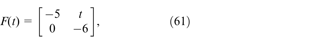
Choose the Hurwitz matrix

$$F(t)=\left[\begin{array}{cc}-5\hfill & t\hfill \\ \multicolumn{1}{c}{0}& -6\hfill \end{array}\right],$$

(61)

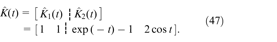
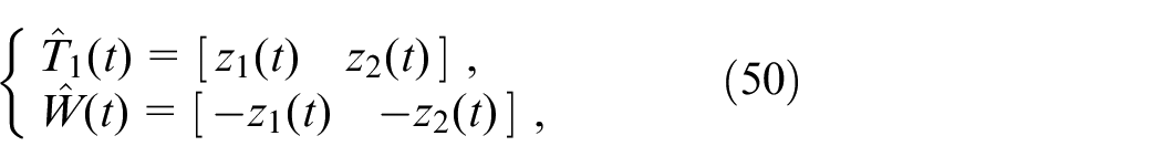
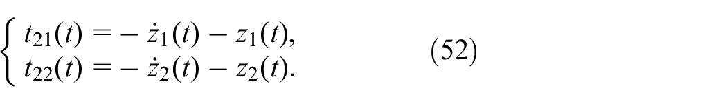
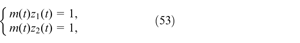
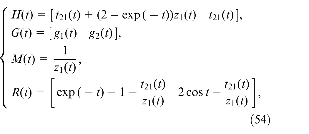
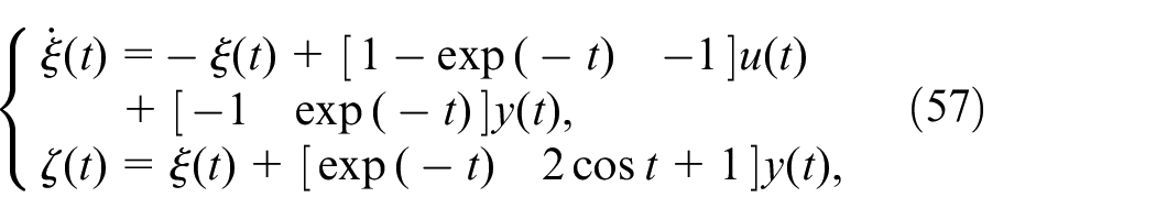
then according to Theorem 3, we obtain the following observer

$$\{\begin{array}{c}\stackrel{·}{\xi }(t)=\left[\begin{array}{cc}-5\hfill & t\hfill \\ \multicolumn{1}{c}{0}& -6\hfill \end{array}\right]\xi (t)+\left[\begin{array}{c}-\exp (-5t)\delta (t)\hfill \\ \multicolumn{1}{c}{\exp (-6t)}\end{array}\right]u(t)\hfill \\ \multicolumn{1}{c}{+\left[\begin{array}{c}\exp (-5t)(\delta (t)+2)\hfill \\ \multicolumn{1}{c}{-\exp (-6t)}\end{array}\right]y(t),}\\ \multicolumn{1}{c}{\zeta (t)=\left[\begin{array}{cc}0\hfill & \sin (t^2)\exp (5t)\hfill \\ \multicolumn{1}{c}{\cos (t^2)\exp (4t)}& \cos (t^2)\exp (5t)\delta (t)\hfill \end{array}\right]\xi (t),}\end{array}$$

(62)

with $\delta (t)=t+\exp (-t)+t\exp (-t)$ .

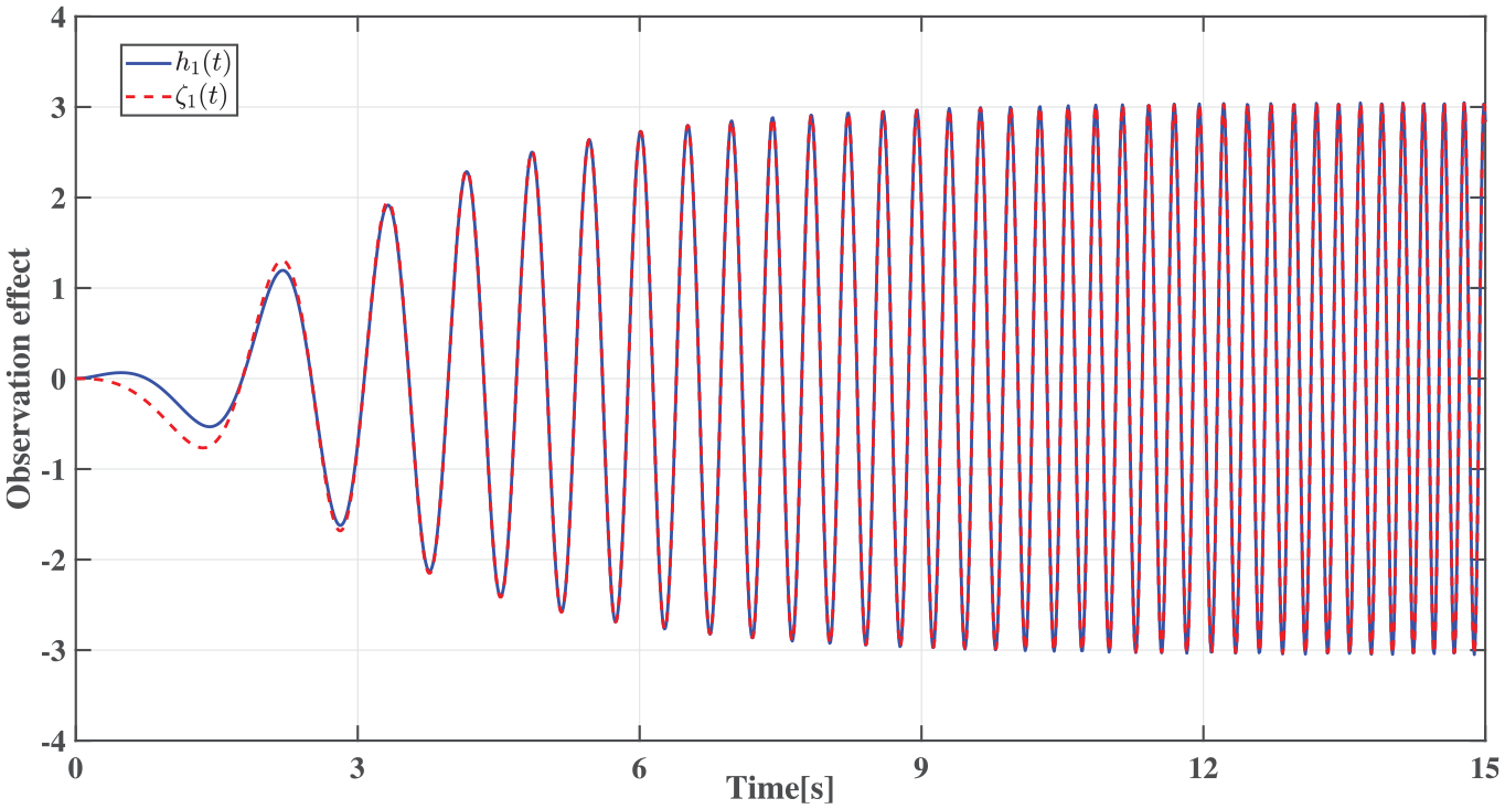
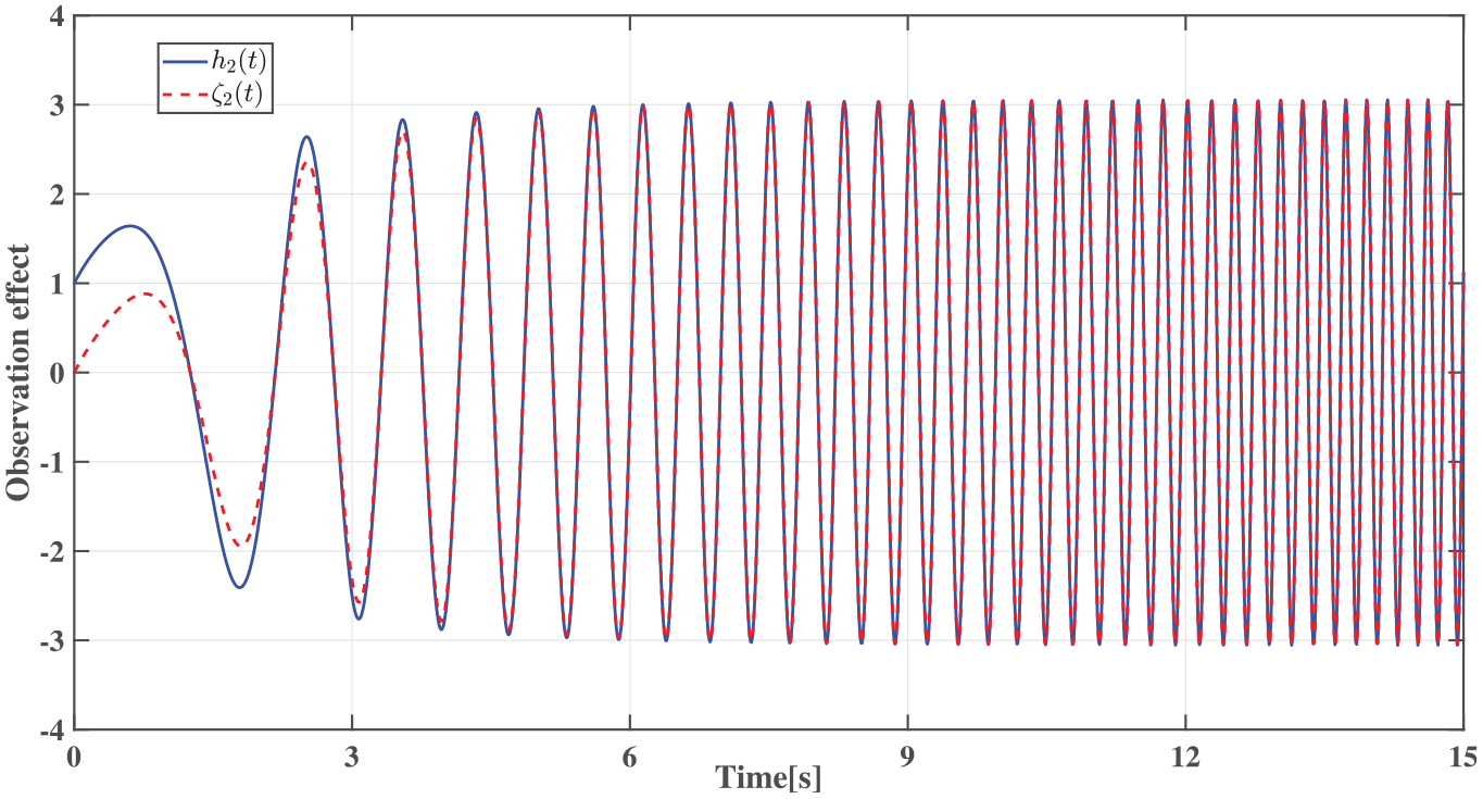
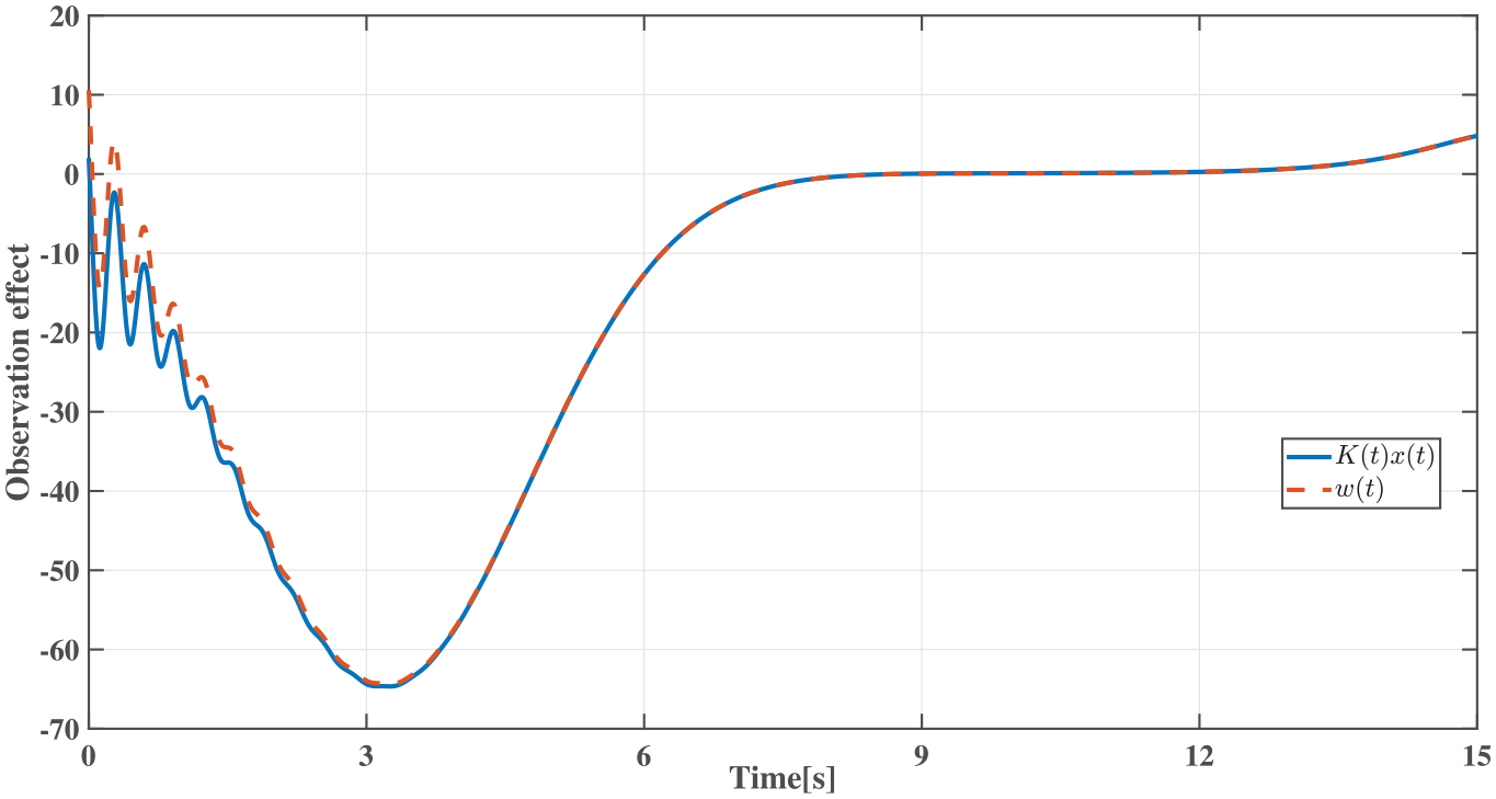
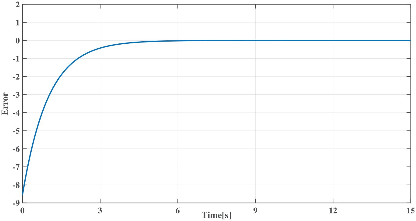
Consider the initial values as $x_1(0)=x_2(0)=x_3(0)=x_4(0)=1$ and ${\xi }_1(0)={\xi }_2(0)=0$ , choose the control input as $u(t)=\sin (t)$ , 0 ≤ t ≤ 15. Then the simulation results are shown in Figures 3 to 5.

Figure 3.

Observation effect of the designed observer.

Figure 4.

Observation effect of the designed observer.

Figure 5.

Estimated error.

Figures 3 to 5 respectively show the observation effect and observed error of the observer. It can be seen from these images that the designed observer can achieve signal tracking well. Compared with the method in Rotella and Zambettakis, ⁴¹ this parametric design avoids the discussion of different cases and reduces the complexity of calculation. Meanwhile, because it does not involve the assumption about stability, the method has a wider applicability and can be applied to any situation.

Aircraft control system

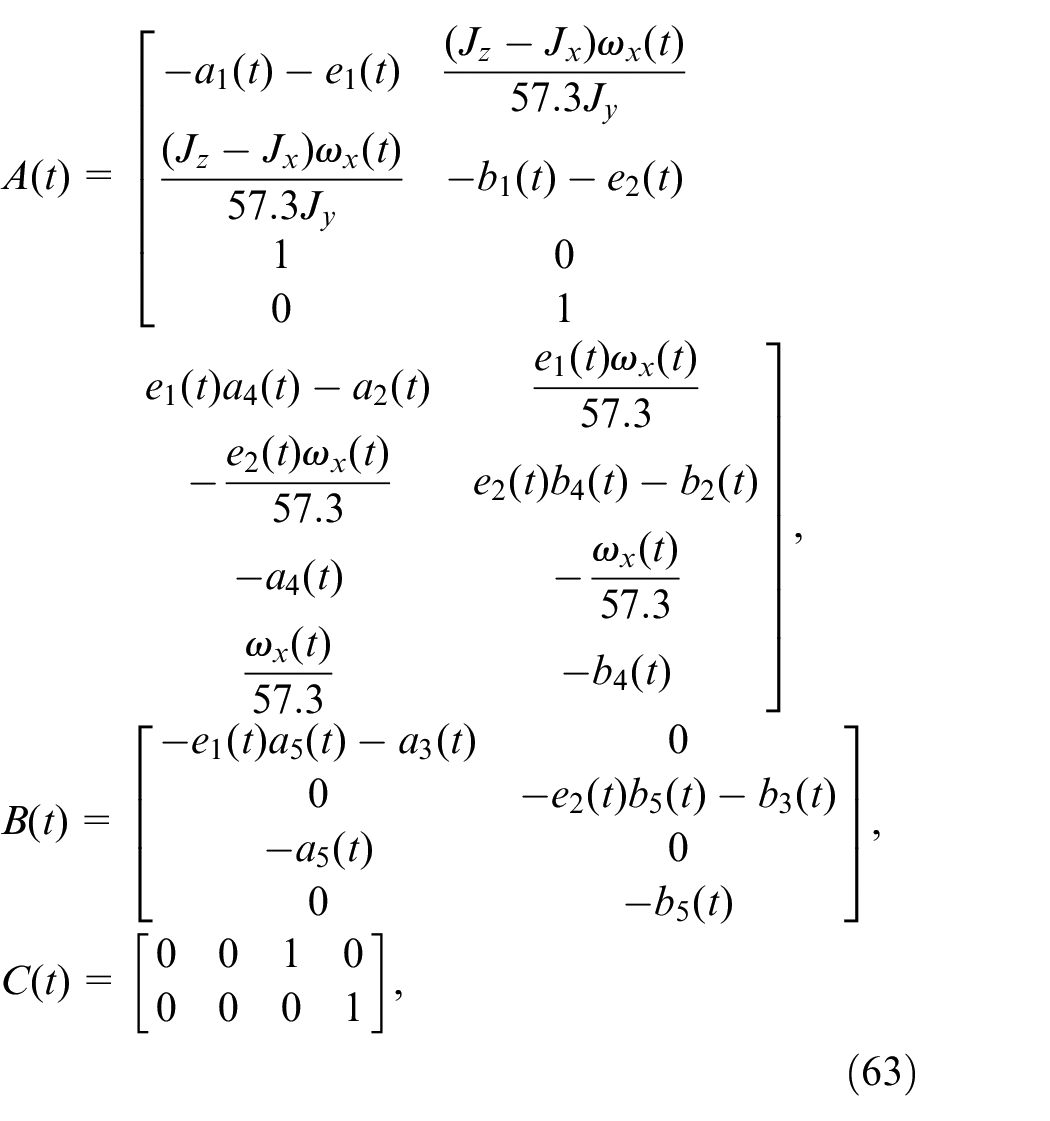
This section takes the ROFO design for BTT aircraft control system as an example to verify the proposed method. Tan et al. ¹¹ presented the mathematical model of BTT missile pitch/yaw channel autopilot as

$$\begin{array}{c}A(t)=[\begin{array}{cc}-a_1(t)-e_1(t)\hfill & \frac{(J_z-J_x){\omega }_x(t)}{57.3J_y}\hfill \\ \multicolumn{1}{c}{\frac{(J_z-J_x){\omega }_x(t)}{57.3J_y}}& -b_1(t)-e_2(t)\hfill \\ \multicolumn{1}{c}{1}& 0\hfill \\ \multicolumn{1}{c}{0}& 1\hfill \end{array}\hfill \\ \begin{array}{cc}{e}_1(t)a_4(t)-a_2(t)\hfill & \frac{e_1(t){\omega }_x(t)}{57.3}\hfill \\ \multicolumn{1}{c}{-\frac{e_2(t){\omega }_x(t)}{57.3}}& e_2(t)b_4(t)-b_2(t)\hfill \\ \multicolumn{1}{c}{-a_4(t)}& -\frac{{\omega }_x(t)}{57.3}\hfill \\ \multicolumn{1}{c}{\frac{{\omega }_x(t)}{57.3}}& -b_4(t)\hfill \end{array}],\hfill \\ B(t)=\left[\begin{array}{cc}-e_1(t)a_5(t)-a_3(t)\hfill & 0\hfill \\ \multicolumn{1}{c}{0}& -e_2(t)b_5(t)-b_3(t)\hfill \\ \multicolumn{1}{c}{-a_5(t)}& 0\hfill \\ \multicolumn{1}{c}{0}& -b_5(t)\hfill \end{array}\right],\hfill \\ C(t)=\left[\begin{array}{cccc}0\hfill & 0\hfill & 1\hfill & 0\hfill \\ \multicolumn{1}{c}{0}& 0\hfill & 0\hfill & 1\hfill \end{array}\right],\hfill \end{array}$$

(63)

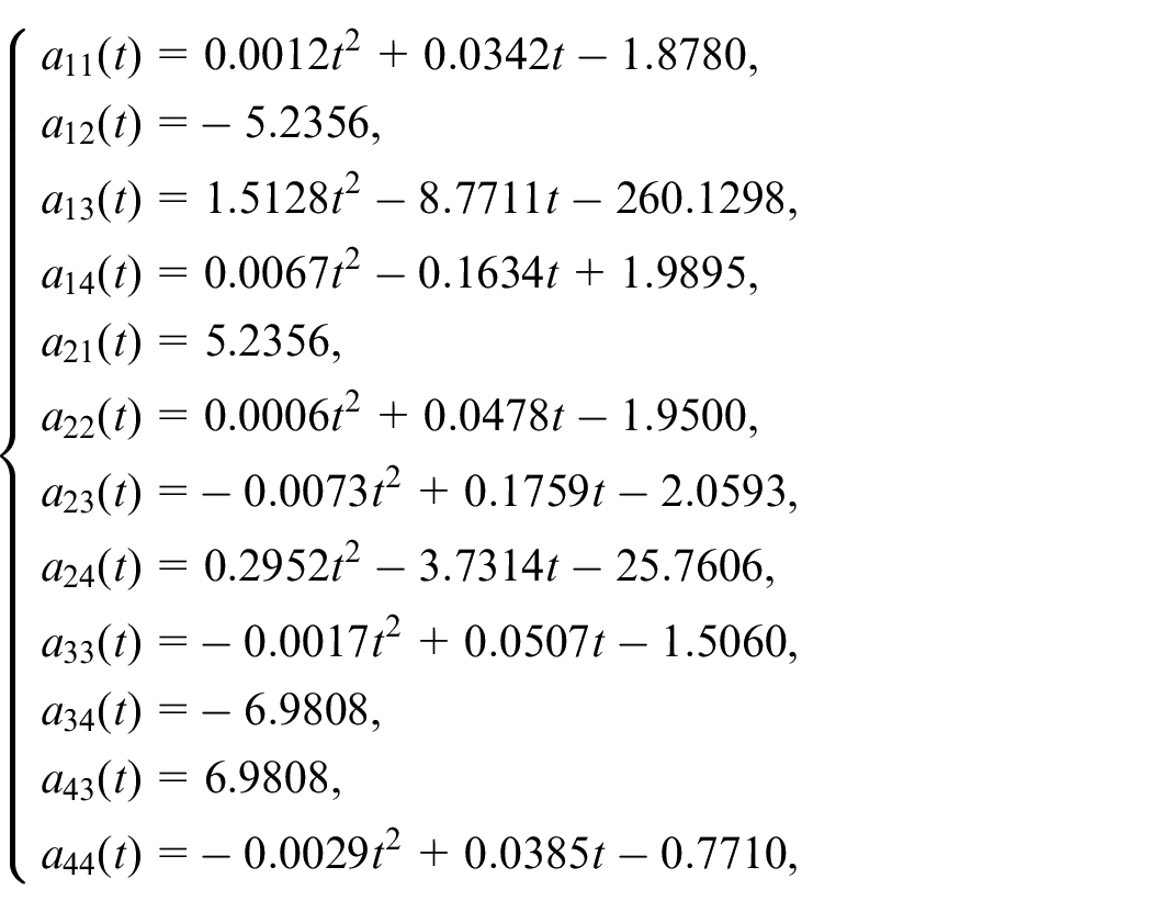
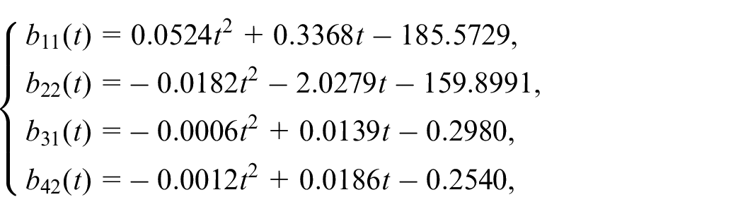
where state $x={[{\omega }_z,{\omega }_y,\alpha ,\beta ]}^{\mathrm{T}}$ , input $u={[{\delta }_z,{\delta }_y]}^{\mathrm{T}}$ , and output $y={[\alpha ,\beta ]}^{\mathrm{T}}$ . The parameters $a_i(t)$ , $b_i(t)$ , $e_i(t)\in \mathbb{P}\mathbb{C}(J,\mathbb{R})$ , which vary with altitude and speed of the missile. ${\omega }_x$ , ${\omega }_y$ , ${\omega }_z$ are the components of angular velocity on the three axes of the projectile coordinate system; $\alpha$ , $\beta$ are the angle of attack and sideslip; ${\delta }_z$ , ${\delta }_y$ represent the yaw angle of the pitch rudder surface and the yaw rudder surface; $J_x$ , $J_y$ , $J_z$ are the moments of inertia of the missile relative to the three axes of projectile coordinate system. The data fitted to matrices $A(t)=[a_{\mathrm{ij}}(t)]$ and $B(t)=[b_{\mathrm{ij}}(t)]$ are given as follows

$$\{\begin{array}{c}{a}_{11}(t)=0.0012t^2+0.0342t-1.8780,\hfill \\ a_{12}(t)=-5.2356,\hfill \\ a_{13}(t)=1.5128t^2-8.7711t-260.1298,\hfill \\ a_{14}(t)=0.0067t^2-0.1634t+1.9895,\hfill \\ a_{21}(t)=5.2356,\hfill \\ a_{22}(t)=0.0006t^2+0.0478t-1.9500,\hfill \\ a_{23}(t)=-0.0073t^2+0.1759t-2.0593,\hfill \\ a_{24}(t)=0.2952t^2-3.7314t-25.7606,\hfill \\ a_{33}(t)=-0.0017t^2+0.0507t-1.5060,\hfill \\ a_{34}(t)=-6.9808,\hfill \\ a_{43}(t)=6.9808,\hfill \\ a_{44}(t)=-0.0029t^2+0.0385t-0.7710,\hfill \end{array}$$

and

$$\{\begin{array}{c}{b}_{11}(t)=0.0524t^2+0.3368t-185.5729,\hfill \\ b_{22}(t)=-0.0182t^2-2.0279t-159.8991,\hfill \\ b_{31}(t)=-0.0006t^2+0.0139t-0.2980,\hfill \\ b_{42}(t)=-0.0012t^2+0.0186t-0.2540,\hfill \end{array}$$

where $a_{31}(t)=a_{42}(t)=1$ and $a_{32}(t)=a_{41}(t)=b_{12}(t)=b_{21}(t)=b_{32}(t)=b_{41}(t)=0$ .

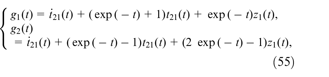
Let the functional

$$K(t)=\left[\begin{array}{cccc}1\hfill & 1\hfill & 0\hfill & 0\hfill \end{array}\right].$$

(64)

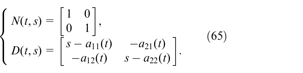
The coefficient matrix $C(t)$ draws in the desired form, thus, the model of BTT aircraft control system is standard form (22) without time-varying transformation. Further, the matrices $N(t,s)$ and $D(t,s)$ satisfying RCF (19) can be obtained as

$$\{\begin{array}{c}N(t,s)=\left[\begin{array}{cc}1\hfill & 0\hfill \\ \multicolumn{1}{c}{0}& 1\hfill \end{array}\right],\hfill \\ \multicolumn{1}{c}{D(t,s)=\left[\begin{array}{cc}s-a_{11}(t)\hfill & -a_{21}(t)\hfill \\ \multicolumn{1}{c}{-a_{12}(t)}& s-a_{22}(t)\hfill \end{array}\right].}\end{array}$$

(65)

Choose the Hurwitz matrix $F(t)=-1$ , denote $M(t)=m(t)$ and

$$Z^{\mathrm{T}}(t)=\left[\begin{array}{cc}{z}_1(t)\hfill & z_2(t)\hfill \end{array}\right].$$

(66)

Then, we have the parametric forms of matrices ${\hat{T}}_1(t)$ , $\hat{W}(t)$ , and ${\hat{T}}_2(t)$ according to equations (32) and (33)

$$\{\begin{array}{c}{\hat{T}}_1(t)=\left[\begin{array}{cc}{z}_1(t)\hfill & z_2(t)\hfill \end{array}\right],\hfill \\ \multicolumn{1}{c}{\hat{W}(t)=\left[\begin{array}{cc}{w}_1(t)\hfill & w_2(t)\hfill \end{array}\right],}\end{array}$$

(67)

where

$$\{\begin{array}{c}{w}_1(t)=-(a_{11}(t)+1)z_1(t)-a_{21}(t)z_2(t),\hfill \\ \multicolumn{1}{c}{w_2(t)=-a_{12}(t)z_1(t)-(a_{22}(t)+1)z_2(t),}\end{array}$$

(68)

and

$${\hat{T}}_2(t)=\left[\begin{array}{cc}{t}_{21}(t)\hfill & t_{22}(t)\hfill \end{array}\right],$$

(69)

where

$$\{\begin{array}{c}{t}_{21}(t)=-(a_{11}(t)+1)z_1(t)-a_{21}(t)z_2(t)-{\stackrel{·}{z}}_1(t),\hfill \\ \multicolumn{1}{c}{t_{22}(t)=-a_{12}(t)z_1(t)-(a_{22}(t)+1)z_2(t)-{\stackrel{·}{z}}_2(t).}\end{array}$$

(70)

Further, the rank condition (34) should be satisfied, that is, the following equation holds

$$\{\begin{array}{c}m(t)z_1(t)=1,\hfill \\ \multicolumn{1}{c}{m(t)z_2(t)=1,}\end{array}$$

(71)

which indicates $z_1(t)=z_2(t)$ , $m(t)=\frac{1}{z_1(t)}$ .

Substituting the above formula into equation (31), yields the following parametric forms of the ROFO as

$$\{\begin{array}{c}H(t)=\left[\begin{array}{cc}{h}_1(t)\hfill & h_2(t)\hfill \end{array}\right],\hfill \\ G(t)=\left[\begin{array}{cc}{g}_1(t)\hfill & g_2(t)\hfill \end{array}\right],\hfill \\ M(t)=\frac{1}{z_1(t)},\hfill \\ R(t)=\left[\begin{array}{cc}-\frac{t_{21}(t)}{z_1(t)}\hfill & -\frac{t_{22}(t)}{z_1(t)}\hfill \end{array}\right],\hfill \end{array}$$

(72)

with

$$\{\begin{array}{c}{h}_1(t)=b_{31}(t)t_{21}(t)+b_{11}(t)z_1(t),\hfill \\ \multicolumn{1}{c}{h_2(t)=b_{42}(t)t_{22}(t)+b_{22}(t)z_1(t),}\\ \multicolumn{1}{c}{g_1(t)={\stackrel{·}{t}}_{21}(t)+(a_{33}(t)+1)t_{21}(t)+a_{43}(t)t_{22}(t)}\\ \multicolumn{1}{c}{+(a_{13}(t)+a_{23}(t))z_1(t),}\\ \multicolumn{1}{c}{g_2(t)={\stackrel{·}{t}}_{22}(t)+a_{34}(t)t_{21}(t)+(a_{44}(t)+1)t_{22}(t)}\\ \multicolumn{1}{c}{+(a_{14}(t)+a_{24}(t))z_1(t),}\end{array}$$

(73)

and

$$\{\begin{array}{c}{t}_{21}(t)=-{\stackrel{·}{z}}_1(t)-(a_{11}(t)+a_{21}(t)+1)z_1(t),\hfill \\ \multicolumn{1}{c}{t_{22}(t)=-{\stackrel{·}{z}}_1(t)-(a_{12}(t)+a_{22}(t)+1)z_1(t),}\end{array}$$

(74)

where $z_1(t)=z_2(t)$ is the parameter can be selected arbitrarily.

Consider the initial values as $x_1(0)=x_2(0)=x_3(0)=1$ , $x_4(0)=-1$ , and $\xi (0)=0$ , without loss of generality, choose the control input as $u_1(t)=u_2(t)=0$ , 0 ≤ t ≤ 15. Let $z_1(t)=1$ , construct the following observer

$$\{\begin{array}{c}\stackrel{·}{\xi }(t)=-\xi (t)\hfill \\ \multicolumn{1}{c}{+[\begin{array}{c}7.2\eta t^4+38.4\eta t^3+0.05489678t^2\hfill \\ \multicolumn{1}{c}{7.2\eta t^4+462\eta t^3-0.0263594t^2}\end{array}}\\ \multicolumn{1}{c}{{\begin{array}{c}+0.28642096t-184.2743352\hfill \\ \multicolumn{1}{c}{-1.90070664t-161.4702424}\end{array}]}^{\mathrm{T}}u(t)}\\ \multicolumn{1}{c}{+[\begin{array}{c}20.4\eta t^4-27\eta t^3+1.5075927t^2\hfill \\ \multicolumn{1}{c}{17.4\eta t^4+1155.2\eta t^3+0.29036102t^2}\end{array}}\\ \multicolumn{1}{c}{{\begin{array}{c}-9.13490736t-216.8379179\hfill \\ \multicolumn{1}{c}{-3.43005724t+8.01713648}\end{array}]}^{\mathrm{T}}y(t),}\\ \multicolumn{1}{c}{\zeta (t)=\xi (t)}\\ \multicolumn{1}{c}{+{\left[\begin{array}{c}0.0012t^2+0.0342t+4.3576\hfill \\ \multicolumn{1}{c}{0.0006t^2+0.0478t-6.1856}\end{array}\right]}^{\mathrm{T}}y(t),}\end{array}$$

(75)

with $\eta ={10}^{-7}$ and the simulation results are plotted in Figures 6 and 7.

Figure 6.

Observation effect of the designed observer.

Figure 7.

Estimated error.

Figures 6 and 7 respectively show the observation effect and observed error of the ROFO. From these two images, we can see that the designed observer can quickly and accurately realize signal tracking, which verifies the effectiveness of this design method in BTT aircraft control system.

Conclusions

Aiming at the ROFO of LTV systems, this paper proposes the existing conditions of the observer and a parameterized design method. Since the gain matrices are given in the form of parameters, when the design requirements change, only the free parameters need to be modified, and other design requirements can be met by using the free parameters. In addition, the designed observer has a lower dimensionality, so it can save costs and is more suitable for engineering practice. Examples including a numerical one, a comparison one and an actual aircraft control one demonstrate the validity of this method.

The future work can be carried out in the following two aspects:

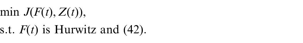
• 1. Optimize the performance of the observer to meet other control requirements. For example, according to the demand, establish an index

$$J=J(F(t),Z(t)),$$

which is a scalar function with respect to the design parameters $F(t)$ and $Z(t)$ , then form an optimization problem of the following form

$$\begin{array}{c}\min J(F(t),Z(t)),\hfill \\ \mathrm{s}.\mathrm{t}.F(t)\mathrm{is}\mathrm{Hurwitz}\mathrm{and}(42).\hfill \end{array}$$

Depending on the specific problem, there may be other constraints added to the above optimization.

• 2. Extend the results to systems with complex characteristics. For instance, time-delay systems, enriching the observer theory.