Sage Journals: Discover world-class research

Abstract

This study considers the visual stabilization problem of nonholonomic mobile robots and proposes a novel optimization stabilization method for visual servo control of nonholonomic mobile robots with monocular cameras fixed onboard. The main idea of the method is to utilize control Lyapunov functions of discrete-time nonlinear systems to design a family of explicit stabilization control laws of the visual servo error system. The parameters of the control laws can indirectly reflect the performance of the visual servo controllers. Then taking account of visibility constraints and actuator limitations, a set of optimal parameters of the control laws is calculated by offline solving a constrained finite horizon optimal control problem. Moreover, the stabilization results on the optimal visual servo controller are established based on the properties of control Lyapunov functions. Finally, some simulation experiments are used to illustrate and evaluate the performance of the visual servo control scheme proposed here.

Keywords

Nonholonomic mobile robots visual servo control control Lyapunov functions nonlinear constrained optimal control

Introduction

Recently, there have been increasing interest in visual feedback-based servo control of mobile robots that commonly focus on nonholonomic kinematic constraints, that is, nonholonomic mobile robots (NMRs). In the study on the visual feedback-based servo control of NMRs, there exist two basic visual servo control problems: visual servo tracking control and visual servo stabilization control of NMRs.^1,2 These visual servo control problems can be formulated as the Cartesian motion control problems of NMRs in the framework of position-based visual servoing of NMRs. This paper works on the visual servo stabilization control of NMRs with monocular vision systems.

Visual stabilization control of NMRs is to use a visual information feedback to drive an NMR from an initial position and pose to a desired position and pose.^1,3 Due to the nonholonomic constraints of NMRs,^3,4 the visual servo stabilization problem of NMRs is more difficult than the visual servo tracking problem of NMRs. Namely, from the viewpoints of control, any time-invariant continuous state feedback control law cannot stabilize a nonholonomic system asymptotically.⁴ To this end, several efforts have been made for the visual servo stabilization control of NMRs.

In early studies, visual servo stabilization of NMRs need position information of the feature points relative to the camera-robot platform.^5–7 Image-based visual servo methods can obtain a priori knowledge from the feature points of a three-dimensional (3D) scene which can directly describe the control objective.¹ In general, the early image-based visual servo controllers calculate the inverse of the image Jacobian of an NMR, which will suffer from the singular in some desired poses of NMRs.^8,9

Lately, several advanced control approaches have been used to design visual servo controllers for stabilization of NMRs. For example, the epipolar geometry technique was exploited to design the two-step visual servo control strategies for stabilization of NMRs.^10,11 Based on the state estimation technique, Lopez-Nicolas et al.¹² presented a hybrid visual servo control strategy for stabilization of NMRs in planar and nonplanar scenes. Without having accurate visual parameters and depth information, Lopez-Nicolas et al.¹³ proposed a two-phase visual servo stabilization controller to stabilize NMRs to the origin. Moreover, a self-adaptive sliding mode controller was considered for stabilization of NMRs¹⁴ and a position-based backstepping visual servo controller was presented for steering control of NMRs.¹⁵ Due to the object occlusion and actuator limitations, visual data obtained from cameras may be lost, which leads to the failure of servoing of NMRs¹⁶ if visual verso control strategies do not take these constraints into account during the controller design. Hence, model predictive control (MPC) has been used to develop the visual servo control schemes of NMRs in recent years, as MPC has advantages to explicitly deal with constraints and optimization control problems.^17–19 For instance, Cao et al.²⁰ proposed an image-based MPC for visual servo stabilization of NMRs with the constraints on visibility and actuators. In order to improve the computational efficiency of visual servo MPC of nonlinear NMRs, Li et al.²¹ employed the neurodynamic optimization technique and He et al.²² adopted the linear matrix inequality technique to design the visual servo MPC of nonlinear NMRs. Nevertheless, the recursive solution of the nonlinear optimization problem of the visual servo MPC generally leads to a heavy computational load for the control system of an NMR and hence, may limit the response speed of the NMR.

In this paper, we propose a novel optimization stabilization method for visual servo stabilization control of NMRs with monocular cameras fixed onboard. First, using control Lyapunov functions (CLF) of discrete-time nonlinear systems,^23,24 a family of explicit feedback control laws is designed to stabilize the visual servo error system of the NMR, where the parameters of the control laws can indirectly reflect the performance of the visual servo controllers. Then in order to take account of the visibility constraints and actuator limitations, the parameters of the control laws are optimized by offline solving a constrained optimal control problem. By the properties of CLFs,^23,24 the stabilization results on the optimal visual servo controller of the NMR are established. With respect to the available visual servoing stabilization strategies, the main contribution of the work is to present an optimal control scheme for visual servo stabilization and constraint satisfaction of the NMR. Note that the nonlinear constrained optimization problem is solved offline and hence will increase the online computational burden of the proposed visual servo controller. Finally, the simulation results evaluate the performance of the visual servo control scheme proposed here.

The rest of the paper is organized as follows. Section “Modeling and problem formulation” presents the visual servoing system of the NMR model and the visual servo control problem. In Section “Visual servo controller design,” the visual servo stabilization controllers of the mobile robot are first designed via CLFs and then the optimal visual servo controller is redesigned by taking the system constraints into account. Some simulation results are given and discussed in Section “Numerical simulations” and Section “Conclusion” concludes the paper.

Modeling and problem formulation

Consider the NMR shown in Figure 1, which is driven independently by two wheels. In the visual servo system of the robot, a monocular camera is used and fixed onboard. Let O-XYZ be the world coordinate system, R-X_rY_r be the coordinate system fixed on the robot and C-X_cY_cZ_c be the camera frame. C is the mass center of the robot. The camera is fixed along the Y_r axis, and the distance between C and the middle of the drive wheels is l. r is the radius of the back wheel and the distance between the back wheels is 2L.

Figure 1.

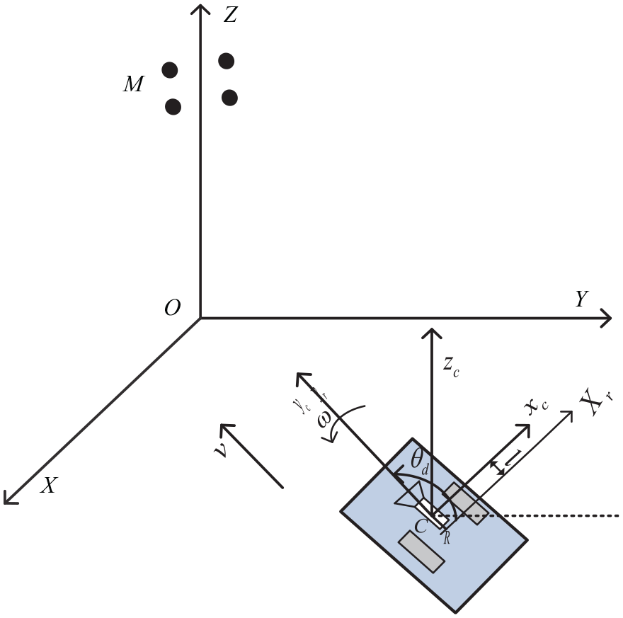
Schematic of a mobile robot with a monocular camera.

Consider the mobile robot with a monocular camera as shown in Figure 1. It is assumed that there is no lateral slip for the mobile robot. Then, the kinematic model of the mobile robot can be expressed as

\frac{dq (t)}{dt} = [\begin{matrix} dx (t) / dt \\ dy (t) / dt \\ d θ (t) / dt \end{matrix}] = [\begin{matrix} - \sin θ (t) & 0 \\ \cos θ (t) & 0 \\ 0 & 1 \end{matrix}] [\begin{matrix} v (t) \\ ω (t) \end{matrix}]

(1)

where q = [x, y, θ]^T is the status of the robot with x and y being the coordinates of the center of the robot and θ being the orientation angle of the mobile robot, and the linear and angular velocities of the mobile robot are represented by v and ω, respectively. Here, v and ω are selected to be the control inputs of the mobile robot.

Assume that the four static feature points shown in Figure 1 are selected to be the target. According to the perspective model,²⁰ the two-dimensional (2D) image coordinate p =[P_x, P_y]^T is derived as

P_{x} = f x_{c} / y_{c}, P_{y} = f z_{c} / y_{c}

(2)

where f is the camera focal length and invariant. Using equation (2), the target point in the 3D Euclidean space is projected to its corresponding point in the image plane.

In visual servo stabilization, visual information is used to drive the mobile robot to a desired image target. When the mobile robot is stabilized to the desired target, the errors of the current and desired images converge to zero. Define the target feature point P as (P_xd, P_yd) and θ_d as the angle at which the mobile robot reaches the target position. Then, the new coordinate is denoted by the image coordinate (s₁, s₂, s₃) as

s = [\begin{matrix} s_{1} \\ s_{2} \\ s_{3} \end{matrix}] = [\begin{matrix} P_{x} / P_{y} \\ - f / P_{y} \\ θ \end{matrix}]

(3)

and the desired coordinates s_d=[P_xd/P_yd − f/P_ydθ_d]^T. Define the visual servo stabilization errors of image coordinate and attitude angle as

e = [\begin{matrix} e_{1} \\ e_{2} \\ e_{3} \end{matrix}] = [\begin{matrix} s_{1} \\ s_{2} \\ s_{3} \end{matrix}] - T_{e} [\begin{matrix} s_{1 d} \\ s_{2 d} \\ s_{3 d} \end{matrix}]

(4)

with the transformation matrix

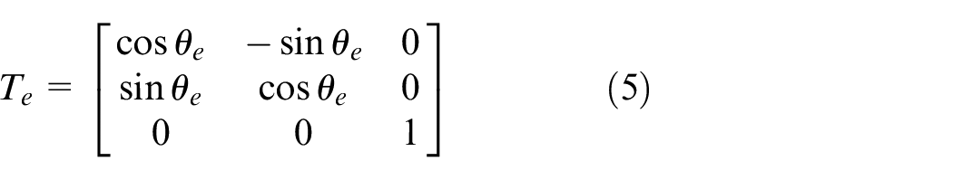
T_{e} = [\begin{matrix} \cos θ_{e} & - \sin θ_{e} & 0 \\ \sin θ_{e} & \cos θ_{e} & 0 \\ 0 & 0 & 1 \end{matrix}]

(5)

where θ_e =θ−θ_d is the angle error of visual servo stabilization for the mobile robot.

Now consider that the relationship between the robot with camera and target point is shown as in Figure 1. Due to the orthogonal transformation between the error vector e and the correlation coordinate system, the differential equation of the error system is obtained by combining equation (1) as²⁰

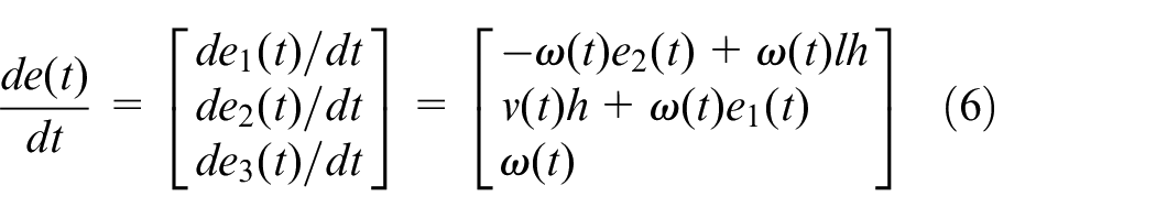
\frac{de (t)}{dt} = [\begin{matrix} d e_{1} (t) / dt \\ d e_{2} (t) / dt \\ d e_{3} (t) / dt \end{matrix}] = [\begin{matrix} - ω (t) e_{2} (t) + ω (t) lh \\ v (t) h + ω (t) e_{1} (t) \\ ω (t) \end{matrix}]

(6)

where h = 1/z_c is a nonzero constant as the height of camera is not zero, that is, z_c ≠ 0. According to equations (4) and (5), the mobile robot will arrive at the target states shown as equation (7) when the error e → 0

s_{1} \to s_{1 d}, s_{2} \to s_{2 d}, θ \to θ_{d}

(7)

Moreover, it is observed from equations (3) and (7) that the image coordinate P_x → P_xd, P_y → P_yd, and θ_e → 0. Hence, the goal of the paper is to design a visual servo stabilizing controller u(t) = u(e(t)) of the mobile robot such that lim_{t → ∞}e(t) = 0 and lim_{t → ∞}u(t) = 0. Here, the tool of CLFs of discrete-time version of equation (6) will be used to find the stabilization controller.

Visual servo controller design

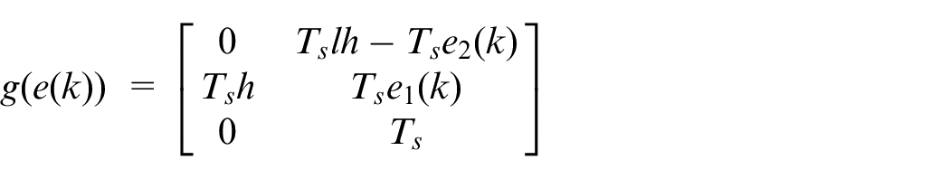
Since visual servo controllers are generally implemented in digital-computer control systems, this paper designs the visual servo stabilizing controller of the NMR based on the discrete-time analog of continuous-time visual servo system (6). By the Euler approximation to equation (6), the discrete-time nonlinear visual servo error model of the NMR can be obtained as the following equation

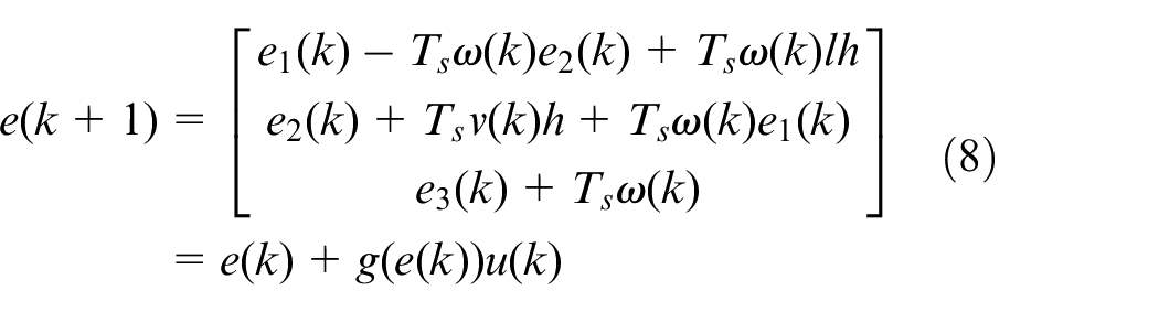
\begin{matrix} e (k + 1) = [\begin{matrix} e_{1} (k) - T_{s} ω (k) e_{2} (k) + T_{s} ω (k) lh \\ e_{2} (k) + T_{s} v (k) h + T_{s} ω (k) e_{1} (k) \\ e_{3} (k) + T_{s} ω (k) \end{matrix}] \\ = e (k) + g (e (k)) u (k) \end{matrix}

(8)

where T_s > 0 is a sufficiently small sampling interval, the control input u =[v ω]^T, and the input matrix

g (e (k)) = [\begin{matrix} 0 & T_{s} lh - T_{s} e_{2} (k) \\ T_{s} h & T_{s} e_{1} (k) \\ 0 & T_{s} \end{matrix}]

Definition 1

Consider the system x⁺ = f(x) + g(x)u, where x⁺ is the successor of x. If there exists a feedback control law K(x) such that the resulting system x⁺ = f(x) + g(x)K(x) is asymptotically stable at the origin, then the system is said to be asymptotically stabilized at the origin by the controller u = K(x).²³

Definition 2

Consider a smooth, proper, and definite positive function V: Rⁿ→R₊, and the system x⁺ = f(x) + g(x)u, where x⁺ is the successor of x.^23,24 If the function V(x) satisfies that

inf_{u} (Δ V (x) = V (x^{+}) - V (x)) < 0, \forall x \in R^{n} \ {0}

(9)

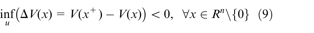
then V(x) is a CLF of the system.

Note that Definition 2 is an extension of Sontag’s result of continuous-time systems to the corresponding discrete-time systems. According to Sontag’s result of continuous-time systems, the control law for the continuous-time system can be obtained.^25,26 Similarly, under some assumptions, there exists a discrete-time feedback control law to stabilize the discrete-time system x⁺ = f(x) + g(x)u if a CLF of the system can be found in prior.²³ However, it is not easy to find a generic, systematic method to construct a CLF of the nonlinear system x⁺ = f(x) + g(x)u. In general, it is assumed that there exists a positive definite matrix P such that V(x) = x^TPx, namely, there exists a quadratic CLF for the nonlinear system.

Consider the discrete-time visual servoing system (8) and define a candidate of CLFs of the system as

V (e) = λ_{1} {e_{1}}^{2} + λ_{2} {e_{2}}^{2} + λ_{3} {e_{3}}^{2} = e^{T} Pe

(10)

where diagonal matrix P = diag{λ₁,λ₂, λ₃} with λ₁, λ₂, λ₃ > 0. For simplicity, let e⁺ is the successor of the current error e, that is, e⁺ = e(k + 1) = e(k) + g(k)u(k). Then, we have the stability result on the discrete-time visual servoing system (8) as follows.

Theorem 1

Consider the discrete-time visual servoing system (8) and the function V(e) in equation (10). There exists a nonempty, invariant set Ŝ and the feedback control law u = [u₁, u₂]^T with

u_{1} = \frac{e_{2}}{h T_{s}} (- 1 + \sqrt{1 - μ_{1}})

(11a)

u_{2} = \frac{λ_{1} lh e_{1} + (λ_{2} - λ_{1}) e_{1} e_{2} + λ_{3} e_{3}}{[λ_{1} {(lh - e_{2})}^{2} + λ_{2} e_{1}^{2} + λ_{3}] T_{s}} (- 1 + \sqrt{1 - μ_{2}})

(11b)

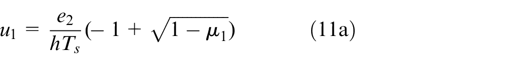
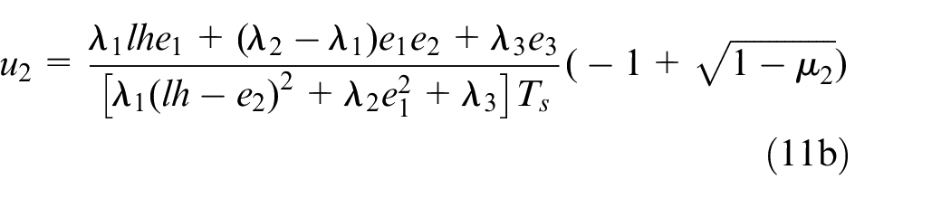
such that V(e) is the local CLF of the system in Ŝ and the system (8) is asymptotically stabilized by equation (11) to the origin for any 0 <µ₁, µ₂ < 1.

Proof

Consider the discrete-time visual servoing system (8) and the function V(e) in equation (10). Taking differential operation of V(e) along the closed-loop trajectories of equation (8), it is derived that

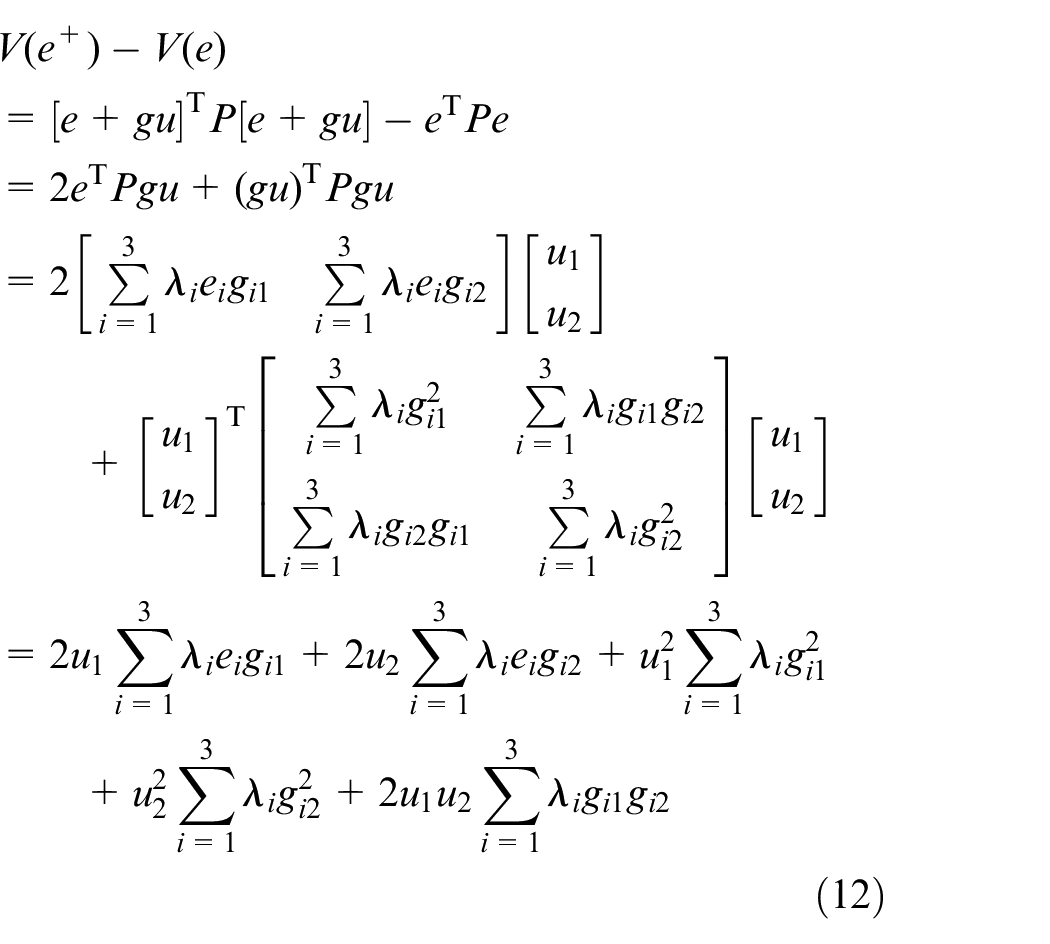
\begin{matrix} V (e^{+}) - V (e) \\ = [e + gu]^{T} P [e + gu] - e^{T} Pe \\ = 2 e^{T} Pgu + (gu)^{T} Pgu \\ = 2 [\begin{matrix} \sum_{i = 1}^{3} λ_{i} e_{i} g_{i 1} & \sum_{i = 1}^{3} λ_{i} e_{i} g_{i 2} \end{matrix}] [\begin{matrix} u_{1} \\ u_{2} \end{matrix}] \\ + {[\begin{matrix} u_{1} \\ u_{2} \end{matrix}]}^{T} [\begin{matrix} \sum_{i = 1}^{3} λ_{i} g_{i 1}^{2} & \sum_{i = 1}^{3} λ_{i} g_{i 1} g_{i 2} \\ \sum_{i = 1}^{3} λ_{i} g_{i 2} g_{i 1} & \sum_{i = 1}^{3} λ_{i} g_{i 2}^{2} \end{matrix}] [\begin{matrix} u_{1} \\ u_{2} \end{matrix}] \\ = 2 u_{1} \sum_{i = 1}^{3} λ_{i} e_{i} g_{i 1} + 2 u_{2} \sum_{i = 1}^{3} λ_{i} e_{i} g_{i 2} + u_{1}^{2} \sum_{i = 1}^{3} λ_{i} g_{i 1}^{2} \\ + u_{2}^{2} \sum_{i = 1}^{3} λ_{i} g_{i 2}^{2} + 2 u_{1} u_{2} \sum_{i = 1}^{3} λ_{i} g_{i 1} g_{i 2} \end{matrix}

(12)

where g_ij is the element in row i and column j of matrix g for i, j = 1, 2, 3. To clarify, let

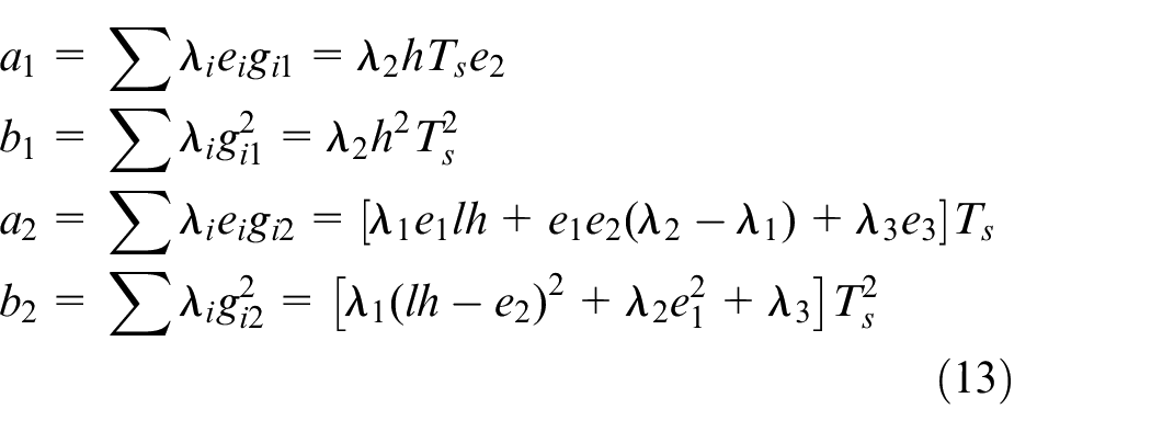
\begin{matrix} a_{1} = \sum λ_{i} e_{i} g_{i 1} = λ_{2} h T_{s} e_{2} \\ b_{1} = \sum λ_{i} g_{i 1}^{2} = λ_{2} h^{2} T_{s}^{2} \\ a_{2} = \sum λ_{i} e_{i} g_{i 2} = [λ_{1} e_{1} lh + e_{1} e_{2} (λ_{2} - λ_{1}) + λ_{3} e_{3}] T_{s} \\ b_{2} = \sum λ_{i} g_{i 2}^{2} = [λ_{1} {(lh - e_{2})}^{2} + λ_{2} e_{1}^{2} + λ_{3}] T_{s}^{2} \end{matrix}

(13)

Substituting equation (13) into equation (12), it is obtained that

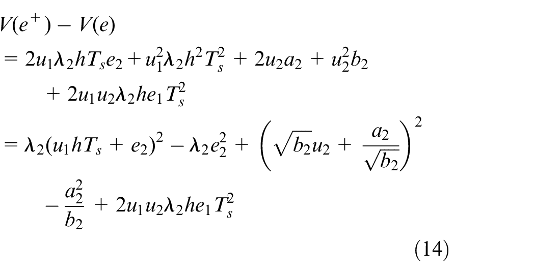
\begin{matrix} V (e^{+}) - V (e) \\ = 2 u_{1} λ_{2} h T_{s} e_{2} + u_{1}^{2} λ_{2} h^{2} T_{s}^{2} + 2 u_{2} a_{2} + u_{2}^{2} b_{2} \\ + 2 u_{1} u_{2} λ_{2} h e_{1} T_{s}^{2} \\ = λ_{2} (u_{1} h T_{s} + e_{2})^{2} - λ_{2} e_{2}^{2} + {(\sqrt{b_{2}} u_{2} + \frac{a_{2}}{\sqrt{b_{2}}})}^{2} \\ - \frac{a_{2}^{2}}{b_{2}} + 2 u_{1} u_{2} λ_{2} h e_{1} T_{s}^{2} \end{matrix}

(14)

Now let us substitute equation (11) into equation (14) and obtain that

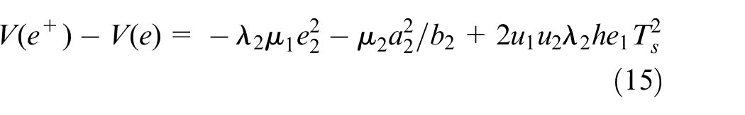
V (e^{+}) - V (e) = - λ_{2} μ_{1} e_{2}^{2} - μ_{2} a_{2}^{2} / b_{2} + 2 u_{1} u_{2} λ_{2} h e_{1} T_{s}^{2}

(15)

For the discrete-time visual servoing system (8), define a set

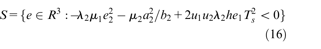
S = {e \in R^{3} : - λ_{2} μ_{1} e_{2}^{2} - μ_{2} a_{2}^{2} / b_{2} + 2 u_{1} u_{2} λ_{2} h e_{1} T_{s}^{2} < 0}

(16)

Note that the origin is the interior of set S and hence, S is nonempty. Pick a number r > 0 such that the set Ŝ ={e∈R³: V(e)≤r}⊆S approaches to the set S as close as possible. Then for any e(k)∈Ŝ at time k≥0, we have that e(k + 1)∈Ŝ since V(e(k + 1))−V(e(k)) < 0. Hence, Ŝ is an invariant set of the discrete-time visual servoing system (8) in closed-loop with equation (11). Moreover, since V(e) is a quadratic CLF of equation (8), the closed-loop system (8) with equation (11) is asymptotically stable to the origin for any 0 <µ₁, µ₂ < 1. This competes the proof of Theorem 1.

Note that from equations (15) and (13), it is observed that the decreasing speed of V(e) in Ŝ relies on the values of λ = (λ₁, λ₂, λ₃) and µ = (µ₁, µ₂). If V(e) is regarded as the energy function of the visual servo system (8) of the mobile robot, then its decreasing speed can reflect the convergence rate of the stabilization error signal e(k). Hence, in principle we can find a set of the optimal parameters λ and µ such that the stabilization error signal e(k) converges in the sense of maximal satisfaction. However, the interplay between these parameter values and the decreasing speed of V(e) is too complex to derive an explicit condition due to strong nonlinearity among them. Moreover, to ensure the target feature points within the camera range and that the mobile robot drives safely and quickly during the servoing process, some constraints must be considered during the design of the controller.

One constraint is the visibility constraint, which keeps the visual features always to be visible. Here the limitations in the errors of e₁ and e₂ are used to formulate the visibility constraint, that is

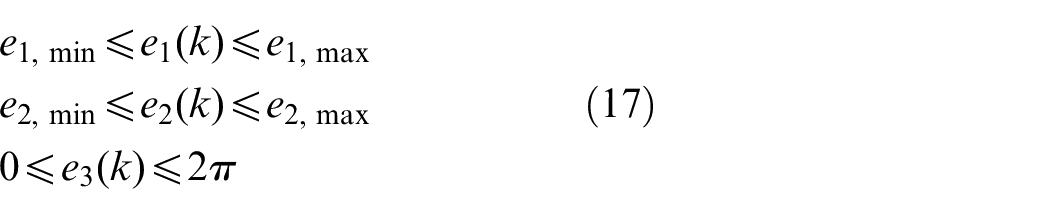
\begin{matrix} e_{1, min} \leq e_{1} (k) \leq e_{1, max} \\ e_{2, min} \leq e_{2} (k) \leq e_{2, max} \\ 0 \leq e_{3} (k) \leq 2 π \end{matrix}

(17)

where e_1,min and e_2,min are the lower limits of e₁ and e₂, respectively, and e_1,max and e_2,max are the upper limits of e₁ and e₂, respectively. The other important constraint is the constraint on the actuator limitations in the velocity and torque variables

\begin{matrix} v_{min} \leq v (k) \leq v_{max} \\ w_{min} \leq w (k) \leq w_{max} \end{matrix}

(18)

where v_min and w_min are the lower limits of velocity v and torque w, respectively, and v_max and w_max are the upper limits of v and w, respectively.

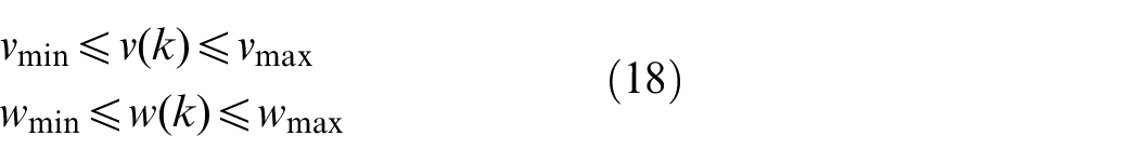
In order to find a set of the optimal parameters λ and µ and to satisfy the constraints (17) and (18), one efficient way is to optimize these parameters according to a predefined cost function.²⁷ To this end, consider the discrete-time visual servoing system (8) and define the cost function over a sufficient large time horizon window N as

J (e (k)) = \sum_{j = k}^{k + N} [e {(j)}^{T} Pe (j) + u {(j)}^{T} Ru (j)]

(19)

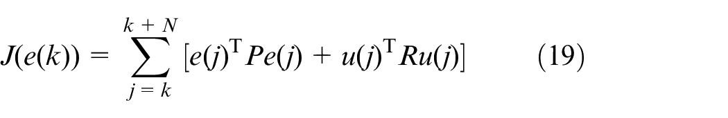
where R > 0 is a weighted matrix on the control input and P = diag{λ₁, λ₂, λ₃} that can be viewed as a weighted matrix on the error. Then for any e(0), define the following optimal control problem to determine the parameters µ

\begin{matrix} min_{μ \in D} J (e (0)) \\ s . t . e (j + 1) = e (j) + g (j) u (e (j), λ, μ) \\ e (j) \in [e_{1, min}, e_{1, max}] \times [e_{2, min}, e_{2, max}] \times [0, 2 π] \\ e (j) \in \hat{S}, u (e (j), λ, μ) \in U, \\ e (j) |_{j = 0} = e (0), \forall j \in [0, N] \end{matrix}

(20)

where function u(e, λ, µ) is given by equation (11), set U is identified by equation (18), and set D = (0.1) × (0.1). From Theorem 1, it is known that there exists at least a set of µ satisfying the constraints in problem (20), that is, the problem is always feasible for any initial state e(0) ∈ Ŝ. Using numerical algorithms, for example, sequence quadratic program (SQP), mesh segmentation, we can derive some optimal solutions to the problem (20).

Let μ^* be the optimal solution to equation (20). Then, the visual feedback-based servo optimal control law of the mobile robot is defined as

\begin{matrix} u (k) = u (e (k), λ, μ^{*} (k)), k \geq 0 \\ = [\begin{matrix} \frac{e_{2} (k)}{h T_{s}} {\bar{μ}}_{1}^{*} \\ \frac{λ_{1} lh e_{1} (k) + (λ_{2} - λ_{1}) e_{1} (k) e_{2} (k) + λ_{3} e_{3} (k)}{[λ_{1} {(lh - e_{2} (k))}^{2} + λ_{2} e_{1}^{2} (k) + λ_{3}] T_{s}} {\bar{μ}}_{2}^{*} \end{matrix}] \end{matrix}

(21)

where ${\bar{μ}}_{i}^{*} = - 1 + \sqrt{1 - μ_{i}^{*}}$ for i = 1 and 2. Note that the optimal controller (21) is a closed-loop feedback control system since it is a function on the current state e(k). Moreover, the computational burden of solving equation (20) may be expensive if the horizon window N is selected to be a large value in order to enhance the performance of the visual servo controller (21). However, the computational burden of online calculating of the control action (21) is not increased during this computing process as it is operated offline.

In what follows, the optimization stabilization result of the visual servoing system (8) with the optimal controller (21) is summarized as Theorem 2.

Theorem 2

Consider the discrete-time visual servoing system (8) and the function V(e) in equation (10). Then, the closed-loop system (8) with the optimal controller (21) is asymptotically stable in the domain of attraction Ŝ.

Proof

The conclusion of Theorem 2 is obtained by directly applying Theorem 1 and the proof of Theorem 2 is omitted here.▪

Numerical simulations

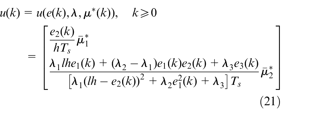
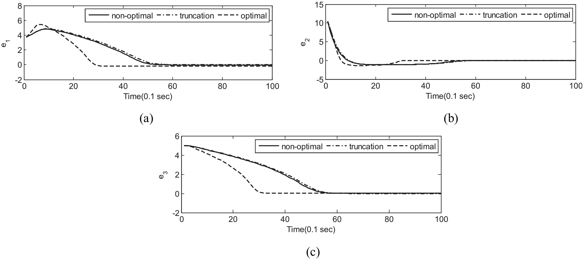
In order to demonstrate the effectiveness of the control scheme, in this section the simulations are executed in MATLAB7.1V. In this study, the physical parameters of the visual servoing system (8) are selected as l = 0.1 m, Z_c = 0.5 m, and T_s = 0.1 s. The constraints (17) and (18) are considered as the following: e_1,min = e_2,min =−5.0, e_1,max = 5.5, e_2,max = 12.5, v_1,max =−v_1,min = 10.0 m/s, and w_1,max = −w_1,min = 3.0 rad/s. In simulation, the initial pose of the mobile robot in O-XYZ is (−1.5, 5.0, 5.0) and the initial error e(k) at time k = 0 is (3.75, 10.5, 5.0). Three simulation experiments are adopted, where the first experiment demonstrates the conclusion of Theorem 1, the second experiment is operated by truncating the controller in the first experiment in order to satisfy the constraints, and the third experiment demonstrates the conclusion of Theorem 2 by comparison of the three experiments.

In the first simulation experiment, the CLF, V(e) of the visual servoing system (8) is selected as V(e) = e₁² + e₂² + e₃², that is, P = diag{1, 1, 1}. The simulation is implemented for the controller in equation (11) without optimizing the parameters (λ,µ) and considering the constraints (17) and (18). The solid lines in Figures 2 and 3 show the simulation results in this experiment. From the solid lines in Figures 2 and 3, one can see that the visual servoing system (8) can converge to the origin, namely, the controller in equation (11) can asymptotically stabilize the visual servoing system. This result shows the feasibility of the proposed approach. Although the convergence velocity of the stabilization errors is slow, the control actions do not satisfy the constraints for all times. In the real application, once some target feature points move out of the camera range during the servoing process, the visual servo controller will be interrupted. Therefore, some constraints must be considered during the controller design.

Figure 2.

Time evolutions of the stabilization errors. (a) Time evolutions of stabilization error e₁. (b) Time evolutions of stabilization error e₂. (c) Time evolutions of stabilization error e_3.

Figure 3.

Time evolutions of the control actions. (a) Time evolutions of linear velocity v. (b) Time evolutions of angular velocity w.

To this end, in the second simulation experiment, the truncation method is used to truncate the violence of the control actions computed from Theorem 1. The dash-dotted lines in Figures 2 and 3 show the simulation results in this experiment. From the dashed–dotted lines in Figures 2 and 3, one can see that although the visual servoing system (8) can converge to the origin, the convergence velocity of the stabilization errors is slower than that of stabilization errors in the first experiment. The main reason is that the truncation of the control actions in this experiment decrease the overall control input of the visual servoing system by comparison with the control input in the first experiment.

In order to optimize the visual servo controller (11) and demonstrate the capability of handling constraints (17) and (18), the nonlinear constrained optimization problem (20) is initialized with the parameters N = 20, P = diag{1, 0.1, 1} and R = diag{0.1, 0.1}. Solving the problem (20), it is derived to be one local optimal solution µ^*= (0.697, 0.897). In order to improve the computational efficiency of solving (20), the Lagrange multiplier method is employed in the MATLAB function “fmincon” as well as the truncation method. Then implementing the optimal visual servo controller (21), we have the simulation results shown as the dashed lines in Figures 2 and 3. It is shown from Figures 2 and 3 that both the stability goal and the visibility constraints are satisfied using this optimal controller. Moreover, the stabilization errors also can be corrected more quickly and tend to zero asymptotically than those obtained by applying the other controllers. These results further illustrate the validity of the proposed control method.

Conclusion

Based on the notion of CLFs of discrete-time nonlinear systems, a novel optimization stabilization method was proposed for visual servo control of NMRs with onboard monocular cameras. By adopting discrete-time CLF of the visual servoing system, a family of explicit stabilization control laws was first designed and then a set of optimal parameters of the control laws was computed by offline solving an optimal control problem by taking account of visibility constraints and actuator limitations. From the simulation results, it was verified that the proposed algorithm was feasible and effective for visual servo control with the NMR. The issues of robust visual servo control and receding horizon optimization visual servo control of constrained NMRs will be pursued along this work in the future work.

Footnotes

Declaration of conflicting interests

The author(s) declared no potential conflicts of interest with respect to the research, authorship, and/or publication of this article.

Funding

The author(s) received no financial support for the research, authorship, and/or publication of this article.

ORCID iD

Kexin Xing

References

Hutchinson

Hager

Corke

. A tutorial on visual servo control. IEEE Trans Robot Autom 1996; 12(5): 651–670.

Liang

Wang

Liu

, et al. Image-based position control of mobile robots with a completely unknown fixed camera. IEEE Trans Automat Contr 2018; 63(9): 3016–3023.

Chen

Wang

, et al. Practical stabilization of uncertain nonholonomic mobile robots based on visual servoing model with uncalibrated camera parameters. In: Proceedings of the 31st Chinese control conference, 25 December 2012, pp. 4406–4411. New York: IEEE.

Goodwine

Zefran

. Feedback stabilization of a class of unstable nonholonomic systems. J Dyn Syst Meas Control 2002; 124: 221–230.

Hashimoto

Noritsugu

. Visual servoing of nonholonomic cart. In: Proceedings of the international conference on robotics and automation, Albuquerque, NM, 25 April 1997, pp. 1719–1724. New York: IEEE.

Masutani

Mikawa

Maru

, et al. Visual servoing for non-holonomic mobile robots. In: Proceedings of international conference on intelligent robots and systems, Munich, 12–16 September 1994, vol. 2, pp. 1133–1140. New York: IEEE.

Pissard-Gibollet

Rives

Applying visual servoing techniques to control a mobile hand-eye system. In: Proceedings of IEEE international conference on robotics and automation, Nagoya, Japan, 21–27 May 1995, pp. 166–171. New York: IEEE.

Conticelli

Allotta

Khosla

. Image-based visual servoing of nonholonomic mobile robots. In: Proceedings of the 38th IEEE conference on decision and control, Phoenix, AZ, 7–10 December 1999, pp. 3496–3501. New York: IEEE.

Burschka

Hager

. Vision-based control of mobile robots. In: Proceedings of the IEEE international conference on robotics and automation, Seoul, South Korea, 21–26 May 2001, pp. 1707–1713. New York: IEEE.

10.

Mariottini

Oriolo

Prattichizzo

. Image-based visual servoing for nonholonomic mobile robots using epipolar geometry. IEEE Trans Robot 2007; 23(1): 87–100.

11.

Cao

Yin

, et al. Visual servo stabilization of nonholonomic mobile robot based on epipolar geometry and 1D trifocal tensor. Chinese J Electron 2013; 22(4): 729–734.

12.

Lopez-Nicolas

Sagues

Guerrero

. Homography-based visual control of nonholonomic vehicles. In: Proceedings of the international conference on robotics and automation, Roma, 10–14 April 2007, pp. 1703–1708. New York: IEEE.

13.

Lopez-Nicolas

Guerrero

Sagues

. Visual control of vehicles using two-view geometry. Mechatronics 2010; 20(2): 315–325.

14.

Lopez-Nicolas

Guerrero

Sagues

. Visual control through the trifocal tensor for nonholonomic robots. Robot Auton Syst 2010; 58(2): 216–226.

15.

Zhang

Fang

Liu

. Motion-estimation-based visual servoing of nonholonomic mobile robots. IEEE Trans ROBOT 2011; 27(6): 1167–1175.

16.

Allibert

Courtial

Chaumette

. Predictive control for constrained image-based visual servoing. IEEE Trans Robot 2010; 26(5): 933–939.

17.

Lucia

Kogel

Zometa

, et al. Predictive control, embedded cyberphysical systems and systems of systems–A perspective. Annu Rev Control 2016; 41: 193–207.

18.

Wang

Sun

. On stability of multiobjective NMPC with objective prioritization. Automatica 2015; 57: 189–198.

19.

Qiu

Luo

. Fuel efficiency-oriented platooning control of connected nonlinear vehicles: a distributed economic MPC approach. Asian J Contr 2019; 21: 1–11.

20.

Cao

Yin

, et al. Predictive control for visual servo stabilization of nonholonomic mobile robots. Acta Automatica Sinica 2013; 39(8): 1238–1245.

21.

Yang

, et al. Vision-based model predictive control for steering of a nonholonomic mobile robot. IEEE Trans Contr Syst Tech 2016; 24(2): 553–564.

22.

. Quasi-min-max predictive control for visual servoing stabilization of mobile robots. Contr Decis. Epub ahead of print July 2019. DOI: 101319; 5/jkzyjc20180743.

23.

Iggidr

Oumoun

Vivalda

. Feedback stabilization of discrete-time nonlinear systems via the control Lyapunov functions. In: Proceedings of the 38th conference on decision & control, Phoenix, AZ, 7–10 December 1999, pp. 2051–2052. New York: IEEE.

24.

Nguyen

Olaru

. A family of piecewise affine control Lyapunov functions. Automatica 2018; 90: 212–219.

25.

Sontag

. A universal construction of Artstein’s theorem on nonlinear stabilization. Syst Control Lett 1989; 13(2): 117–123.

26.

Khalil

. Nonlinear systems. 3rd ed. Upper Saddle River, NJ: Prentice Hall, 2002.

27.

Song

. Optimized-based stabilization of constrained nonlinear systems: a receding horizon approach. Asian J Control 2014; 16(6): 1693–1701.

Visual servo optimization stabilization of nonholonomic mobile robots based on control Lyapunov functions

Abstract

Keywords

Introduction

Modeling and problem formulation

Visual servo controller design

Definition 1

Definition 2

Theorem 1

Proof

Theorem 2

Proof

Numerical simulations

Conclusion

Footnotes

Declaration of conflicting interests

Funding

ORCID iD

References