
Abstract
Exploratory graph analysis (EGA) is a commonly applied technique intended to help social scientists discover latent variables. Yet, the results can be influenced by the methodological decisions the researcher makes along the way. In this article, we focus on the choice regarding the number of factors to retain: We compare the performance of the recently developed EGA with various traditional factor retention criteria. We use both continuous and binary data, as evidence regarding the accuracy of such criteria in the latter case is scarce. Simulation results, based on scenarios resulting from varying sample size, communalities from major factors, interfactor correlations, skewness, and correlation measure, show that EGA outperforms the traditional factor retention criteria considered in most cases in terms of bias and accuracy. In addition, we show that factor retention decisions for binary data are preferably made using Pearson, instead of tetrachoric, correlations, which is contradictory to popular belief.
Introduction
Social scientists often aim to explain behavioral phenomena using both observable and unobservable variables. To this aim, they frequently employ exploratory factor analysis (EFA), a technique that is used to discover and understand latent variables. With the goal of generating theory, researchers aim to explain a good portion of the variance among the originally measured
An important choice in the factor analytic process is the number of factors to retain. Extracting too few factors compresses variables into a smaller factor space leading to loss of information, neglect of important factors, distorted results, and increased error in the loadings. Extracting too many diffuses variables across a larger space. This results in splitting of factors, limiting interpretation, or trivial factors (Auerswald & Moshagen, 2019; Hayton et al., 2004).
Multiple studies have reviewed the use of EFA in psychological research (e.g., Conway & Huffcutt, 2003; Fabrigar et al., 1999; Ford et al., 1986; Goretzko et al., 2019; Henson & Roberts, 2006; Norris & Lecavalier, 2010). Almost all of these studies conclude that the choice regarding the number of factors to retain has been dominated by the standard options in statistical software. Goretzko et al. (2019), for example, find that 55% of studies still employ the Kaiser criterion and 46% the scree test. While it is important to choose a criterion that performs well in all circumstances, other methods, such as parallel analysis, or, more recently, exploratory graph analysis (EGA; Golino & Epskamp, 2017; Golino, Shi, et al., 2020) are often overlooked by applied researchers.
Research also increasingly relies on simpler response formats, such as questionnaires with binary responses, to increase response rates and decrease the danger of response bias. Instead of providing statements accompanied by a Likert-type scale, researchers simply ask the respondents whether or not they agree with the statement by either indicating “No” or “Yes”. For example, when asking respondents to position a brand with regard to certain characteristics, a question could be “Indicate to what extent you agree with the following statement: Brand X is innovative.” Dolnicar et al. (2011) show that a binary response format saves respondent time and is perceived simpler while not influencing reliability or interpretations of results. Yet, the validity of the results following from the application of traditional factor retention criteria to binary data has not been studied widely.
Several recent articles (see Table 1) have studied how the choice of factor retention criterion influences the correctness of the results. Most of these concentrate on continuous data (Auerswald & Moshagen, 2019; Crawford et al., 2010; Goretzko & Bühner, 2020; Li et al., 2020; Ruscio & Roche, 2012) or limit their focus to the assessment of parallel analysis and its variations (Cho et al., 2009; Green et al., 2016; Lim & Jahng, 2019). Only Yang and Xia (2015) assess various criteria in the context of ordinal and binary data, yet do not take into account the performance of EGA. The studies by Golino and Epskamp (2017) and Golino, Shi, et al. (2020) resemble our current investigation most closely, yet these authors do not determine the influence of the use of regular Pearson correlations for analyzing binary data, nor do they consider the performance of revised parallel analysis (Green et al., 2012). In addition, both studies simulate their data according to the factor model and do not allow for the influence of “minor factors” which model the “lack-of-fit” commonly found when fitting the factor model to real-world data (Hong, 1999; MacCallum & Tucker, 1991; Tucker et al., 1969).
Overview of Recent Studies Reviewing Factor Retention Criteria.
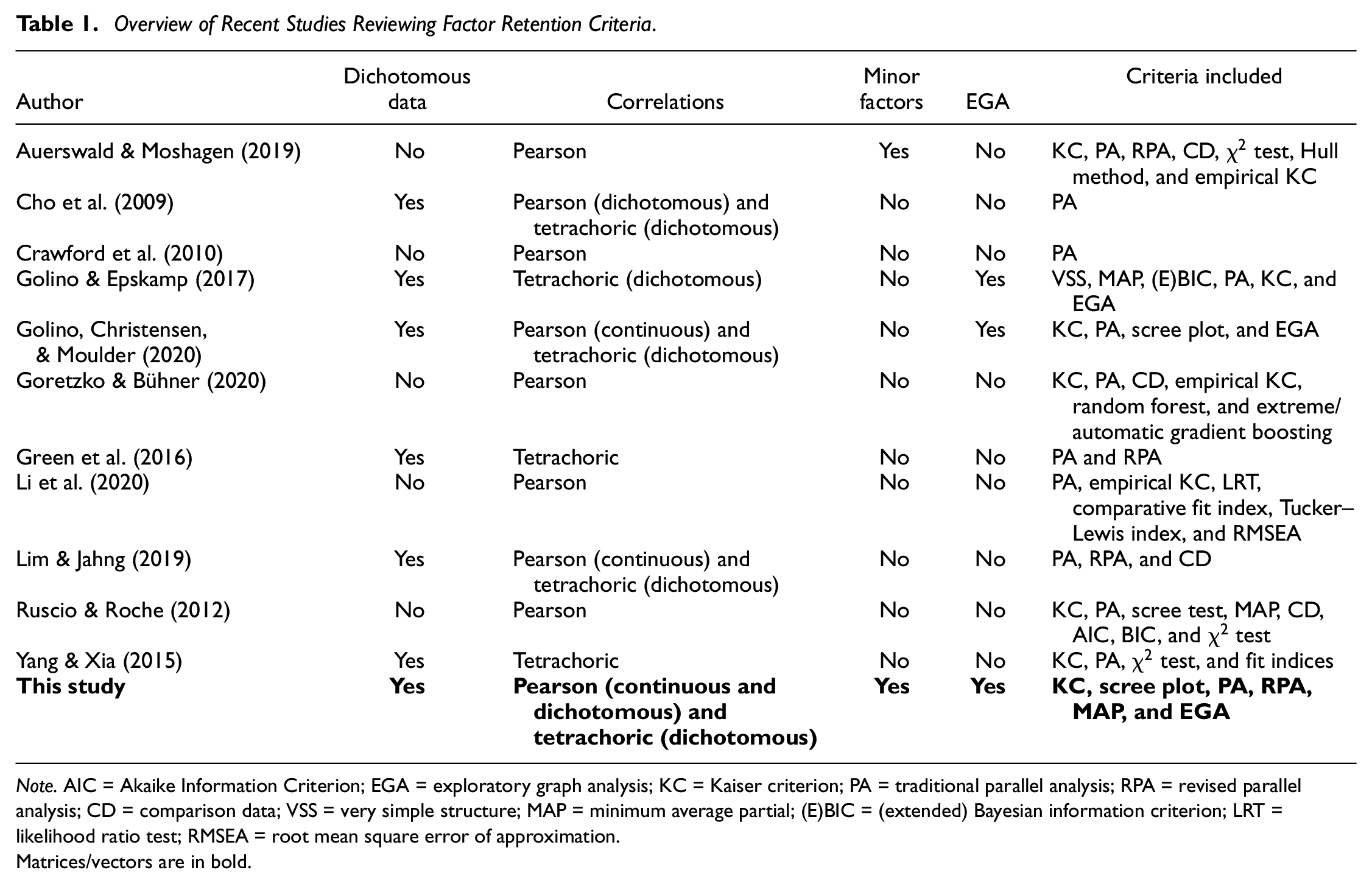
Note. AIC = Akaike Information Criterion; EGA = exploratory graph analysis; KC = Kaiser criterion; PA = traditional parallel analysis; RPA = revised parallel analysis; CD = comparison data; VSS = very simple structure; MAP = minimum average partial; (E)BIC = (extended) Bayesian information criterion; LRT = likelihood ratio test; RMSEA = root mean square error of approximation.Matrices/vectors are in bold.
In what follows, we introduce the general factor analysis model, its assumptions and extensions for binary data, and discuss the various factor retention criteria considered more elaborately. Next, we illustrate the data simulation procedure and detail the fixed and variable input parameters. We then present the results of the study and discuss their impact. Limitations and opportunities for future research are discussed last.
Factor Analysis
Fundamental Equations
Underlying factor analysis is the assumption that the same latent variables influence the observed set of manifest variables, thereby causing a correlation structure between them (Bartholomew et al., 2008; Johnson & Wichern, 2002; Mulaik, 2009). Suppose we have

Or, in matrix notation

where
Under certain assumptions, the fundamental theorem of factor analysis then states that the correlation matrix of the standardized observed variables

Given that the matrix
Factor Analysis for Binary Data
The model presented in Equation 1 is, however, not suited for binary variables. Pearson correlations are generally improper for studying dichotomous data: Given that we assume both
Factor Retention Criteria
Previous research (e.g., Conway & Huffcutt, 2003; Fabrigar et al., 1999; Ford et al., 1986; Goretzko et al., 2019; Henson & Roberts, 2006; Norris & Lecavalier, 2010) has shown that the most frequently employed methods are the eigenvalue-greater-than-one rule or Kaiser criterion (Kaiser, 1960), scree plot (Cattell, 1966), parallel analysis (Horn, 1965), and minimum average partial method (Velicer, 1976). In this section, we will introduce all of these methods, along with their extensions. In addition, we will also look at the recently developed EGA (Golino & Epskamp, 2017; Golino, Shi, et al., 2020).
Kaiser Criterion
The majority of factor extraction criteria rely on the eigenvalues of the observed correlation matrix. Starting from the factor model in Equation 1 and the corresponding decomposition of the correlation matrix

where
Scree Plot
Cattell’s scree test (Cattell, 1966) involves plotting the sequential eigenvalues from the factor analysis procedure and looking for the “elbow” in the graph. This point defines the optimal number of factors to retain.
The subjectivity involved in this criterion is, however, high as it is merely based on a visual interpretation (Hayton et al., 2004). Raîche et al. (2013) therefore devise several nongraphical solutions to this problem, among which the acceleration factor, which closely aligns with the intuition behind the scree test. More specifically, Raîche et al. (2013) state that the elbow of the plot corresponds to the point where the slope of the curve changes most abruptly. The number of factors to retain is the point preceding the number of factors where the acceleration factor is maximal.
This solution does, however, not take into account that the eigenvalues of the retained factors could be so small as to render them useless. In addition, the criterion is therefore often evaluated in combination with the Kaiser criterion discussed above. This amounts to taking the minimum of the factors indicated by either one of these rules (Raîche et al., 2013). Again the eigenvalues used for these tests come from the components analysis of the correlation matrix.
Traditional Parallel Analysis
Because of sampling error, eigenvalues can be larger than one even if no additional factor is present. This causes the Kaiser criterion to regularly overextract (Auerswald & Moshagen, 2019).
Parallel analysis, originally presented by Horn (1965), illustrates the concept of using the eigenvalues of random data with no underlying factor structure to determine the optimal number of factors to retain. The procedure starts by simulating
Given that parallel analyisis using principal components analysis has often been found to outperform its common factor counterpart, we will be using the former method (Auerswald & Moshagen, 2019; Crawford et al., 2010; Golino, Shi, et al., 2020; Ruscio & Roche, 2012).
Revised Parallel Analysis
Green et al. (2012) argue that the original approach to parallel analysis is more of a heuristic than a mathematically rigorous procedure. They reason that the method described above only yields the appropriate reference distribution for the first empirical eigenvalue: The eigenvalue for deciding upon the
As recommended by Green et al. (2012), we apply the revised parallel analysis both with and without the addition of the Kaiser criterion and based on the 95th percentile of eigenvalues. In addition, recent simulations by Auerswald and Moshagen (2019) have shown that if based on the common factor model, the method severely underperforms. Therefore, implementation in this study is based on principal components analysis.
Minimum Average Partial
Velicer (1976) proposes choosing the optimal number of factors based on the minimum average squared partial correlation. Given

which is the average of the squared partial correlations (only including the off-diagonal elements) after the first

in which case no components are extracted (Velicer, 1976). This means that factors are retained as long as the variance left in the partial (co)variance matrix is systematic in nature (Hayton et al., 2004).
EGA
Unlike most methods discussed above, EGA, developed by Golino and Epskamp (2017), does not rely on the eigenvalues of the (reduced) correlation matrix. It, therefore, is not impacted by a preliminary choice of model (common components or factor analysis) or method (principal components, principal axis factor, maximum likelihood, etc.) and any problems this might entail (such as violations of assumptions). Instead, it models the variables as a multivariate normally distributed network (i.e., a Gaussian graphical model or GGM; Golino & Epskamp, 2017). The algorithm represents the manifest variables as a network of nodes connected by weighted edges and proposes the latent variables from the factor model will cause these nodes to cluster together. Golino and Epskamp (2017) use the inverse variance–covariance matrix between manifest variables to represent the edge weights, which, after standardization, can be interpreted as a matrix of partial correlation coefficients. While the variance–covariance matrix can be inverted directly, doing so entails larger standard errors and unstable parameters in small data sets due to overfitting. Therefore, Golino and Epskamp (2017) propose the use of the LASSO to estimate this matrix. As this type of penalized maximum likelihood estimates many coefficients to be exactly zero, it guards against overfitting. The tuning parameter of this method, that controls the degree of sparsity, is estimated by minimizing the extended Bayesian information criterion (Golino & Epskamp, 2017; Golino, Shi, et al., 2020).
The Walktrap algorithm then allows detecting of the number of dimensions in the network. If we let

with

we can be further expand the previous equation to include the distance between two communities as

The algorithm starts with each node as a cluster, calculating the distances between them and joining two clusters at a time, each time recalculating the distances between the nodes and the clusters. The choice of which clusters to merge depends on the change in variation

This variation is minimized in each step.
The best number of clusters is chosen based on the number that maximizes modularity. If we have a network with two clusters

This criterion penalizes network structures with only one cluster. As a consequence, this algorithm is not expected to work well for unidimensional structures. Golino, Shi, et al. (2020) therefore start their improved version of the algorithm by simulating a unidimensional data set with four variables and loadings of 0.70 and bind these simulated data with the user-provided data. This prevents the penalization inherent to the Walktrap algorithm for single cluster solutions (Golino, Shi, et al., 2020). Implementation of this algorithm is done by means of the EGAnet package in R (Golino, Christensen, & Moulder, 2020).
Simulation Setup
Population and Data Generating Process
In this section, we describe the procedure that generates population correlation matrices from which the data for factor analysis are sampled. This procedure relies on the simulation model, proposed by Tucker et al. (1969), that shares many features with the formal model of factor analysis discussed previously. Both models assume the existence of a major domain that contains
In this study, we require the major factor loadings to have a perfect simple structure, following the applications of this method in literature (Briggs & MacCallum, 2003; De Winter & Dodou, 2012, 2016; MacCallum et al., 1999; Pearson & Mundform, 2010). This is a factor solution for which each factor only has a subset of variables with high loadings and each variable has high loadings on only some factors, but preferably only one (Fabrigar et al., 1999).
A matrix with loadings on the several other, unmodelled, minor factors is generated by drawing independent random standard normal deviates (
Given this correlation matrix

where
Scenarios
Several parameters will be varied throughout the study, their combinations constitute the different scenarios that will be analyzed. More specifically, sample size
Variable Input Parameters.
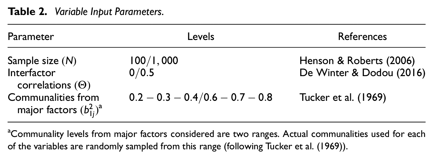
Communality levels from major factors considered are two ranges. Actual communalities used for each of the variables are randomly sampled from this range (following Tucker et al. (1969)).
Directly as continuous data using a Pearson correlation matrix;
After dichotomization resulting in a 50–50 split between zeroes and ones
After dichotomization resulting in a 75–25 split between zeroes and ones
The comparison of the results between the continuous and dichotomous analyses allows us to assess the impact of the dichotomization on the results of the factor analytic process. Academic research usually sets the cut-off for this dichotomization at
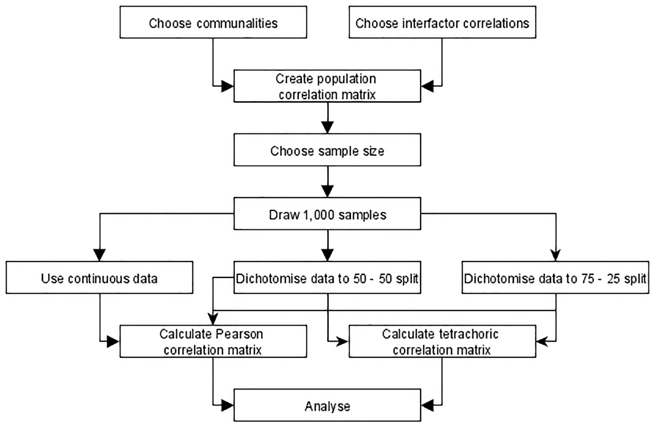
Schematic Representation of the Data Simulation Procedure.
In addition, some parameters will remain fixed throughout the study. Their values will not be changed as to assess their impact (Table 3). We keep the number of variables
Fixed Input Parameters.
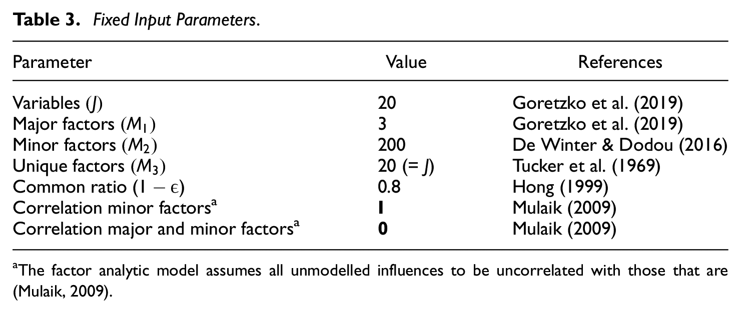
The factor analytic model assumes all unmodelled influences to be uncorrelated with those that are (Mulaik, 2009).
The communalities from the minor factors are always set to half of the square root of the variance not explained by the communalities from the major factors, following Tucker et al. (1969). The rest of the variance is taken to be explained by the unique variances. For more info on the data generation process, please refer to the Supplementary Materials.
Analysis
Data and accompanying correlation matrices are generated as described in Figure 1 and analyzed using nine different factor retention criteria. Every population correlation matrix represents a hypothetical population factor model characterized by certain conditions that applied researchers want to unravel. Yet, researchers only observe one sample from this population at a time. We draw
Hereafter, each of the criteria will be abbreviated in the following way: EV: Kaiser criterion, AF: acceleration factor alternative to the scree plot, AFEV: acceleration factor combined with the Kaiser criterion, PAM: parallel analysis based on the mean eigenvalues, PA95: parallel analysis based on the 95th percentile of eigenvalues, RPA: revised parallel analysis based on the 95th percentile of eigenvalues, RPAEV: revised parallel analysis based on the 95th percentile of eigenvalues combined with the Kaiser criterion, MAP: minimum average partial method, and EGA: exploratory graph analysis.
Results
Continuous Data
The linear and logistic regression models can be used to predict the expected bias and probability of correctly predicting the number of factors for each of the nine criteria. The results of this procedure for continuous data are displayed in Figure 2 and Table 4.
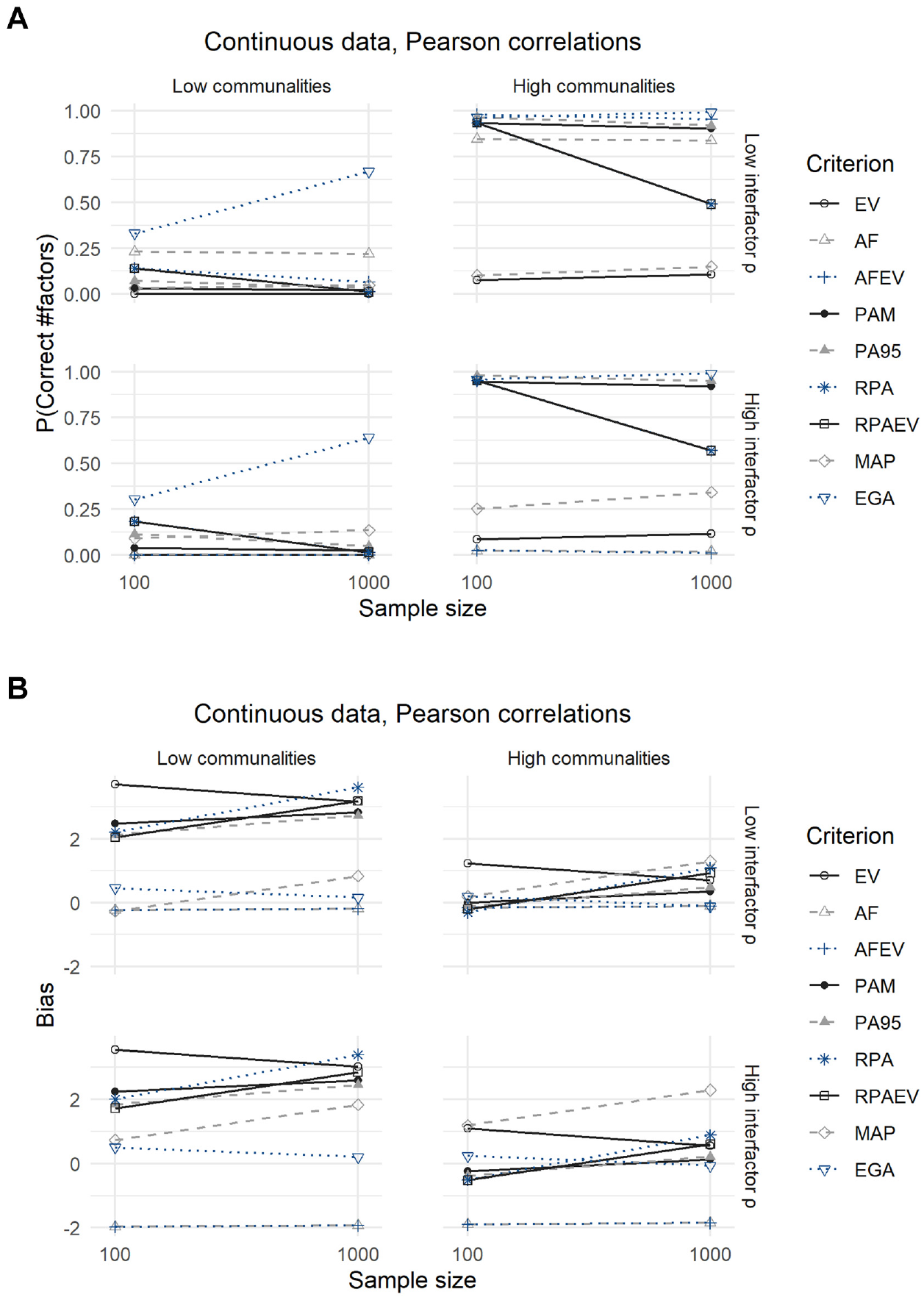
Results for Continuous Data: (A) Expected Probability of Correctly Predicting the Number of Factors and (B) Expected Bias.
Results for Continuous Data.
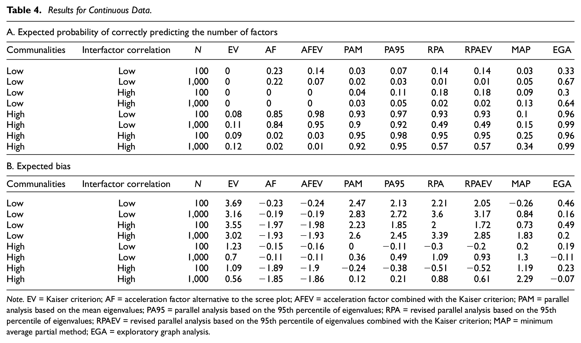
Note. EV = Kaiser criterion; AF = acceleration factor alternative to the scree plot; AFEV = acceleration factor combined with the Kaiser criterion; PAM = parallel analysis based on the mean eigenvalues; PA95 = parallel analysis based on the 95th percentile of eigenvalues; RPA = revised parallel analysis based on the 95th percentile of eigenvalues; RPAEV = revised parallel analysis based on the 95th percentile of eigenvalues combined with the Kaiser criterion; MAP = minimum average partial method; EGA = exploratory graph analysis.
The well-known EV criterion is among the worst performing in each of the scenarios as it never correctly predicts the number of factors to retain in case communalities from major factors are low. The expected probability of a correct prediction rises only slightly, to approximately 0.10, when communalities from major factors or sample sizes increase. The same can be said for the MAP, AF, and AFEV criteria, with the exception that the latter two perform seemingly well in scenarios defined by high communalities from major factors and low interfactor correlations where they reach expected probabilities of a correct prediction of 0.84 to 0.98. At the other end of the spectrum is the EGA criterion, which has the highest expected hit rates of all criteria in each of the scenarios. Even in challenging circumstances of low communalities from major factors where most other criteria fail, does the EGA method achieve a reasonable expected accuracy of around 0.65 with larger sample sizes. Results regarding other criteria are less clear-cut as their performance depends on the scenarios in which they are employed. Both PAM and PA95 perform well in situations with high communalities from major factors, approximating the same expected accuracy as the EGA criterion in the range 0.90 to 0.98. When variables are only weakly influenced by their common factors, both methods underperform and have expected accuracies similar to that of the EV criterion in the range 0.02 to 0.11. Finally, both RPA and RPAEV show patterns contrasting those of other criteria, with expected accuracies decreasing as sample sizes increase. When faced with small samples, RPA and RPAEV approach the performance of the EGA, especially when communalities from major factors are high. In larger samples their accuracy decreases significantly to 0.57 in the best case scenario of high communalities from major factors and high interfactor correlations.
The second panel of Figure 2 and Table 4 indicates to which extent the underperforming criteria favor over- or underextraction (indicated by positive and negative expected biases, respectively). The EV criterion almost always overextracts, a result also discussed Hayton et al. (2004), and at its worst predicts almost four factors more than optimal. This is in contrast to the AF and AFEV criteria, which tend to favor less factors when they underperform as their expected biases are all negative. The PAM, PA95, RPA, RPAEV, and MAP commonly overestimate the optimal number of factors when they do indicate the incorrectness of the number of factors. Again, the expected bias of the EGA criterion is small in all scenarios.
Dichotomous Data (50–50 Split)
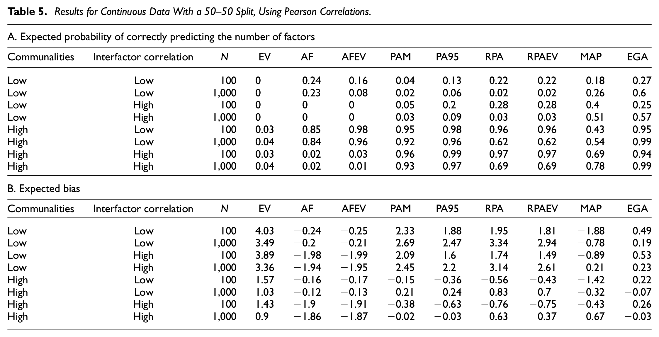
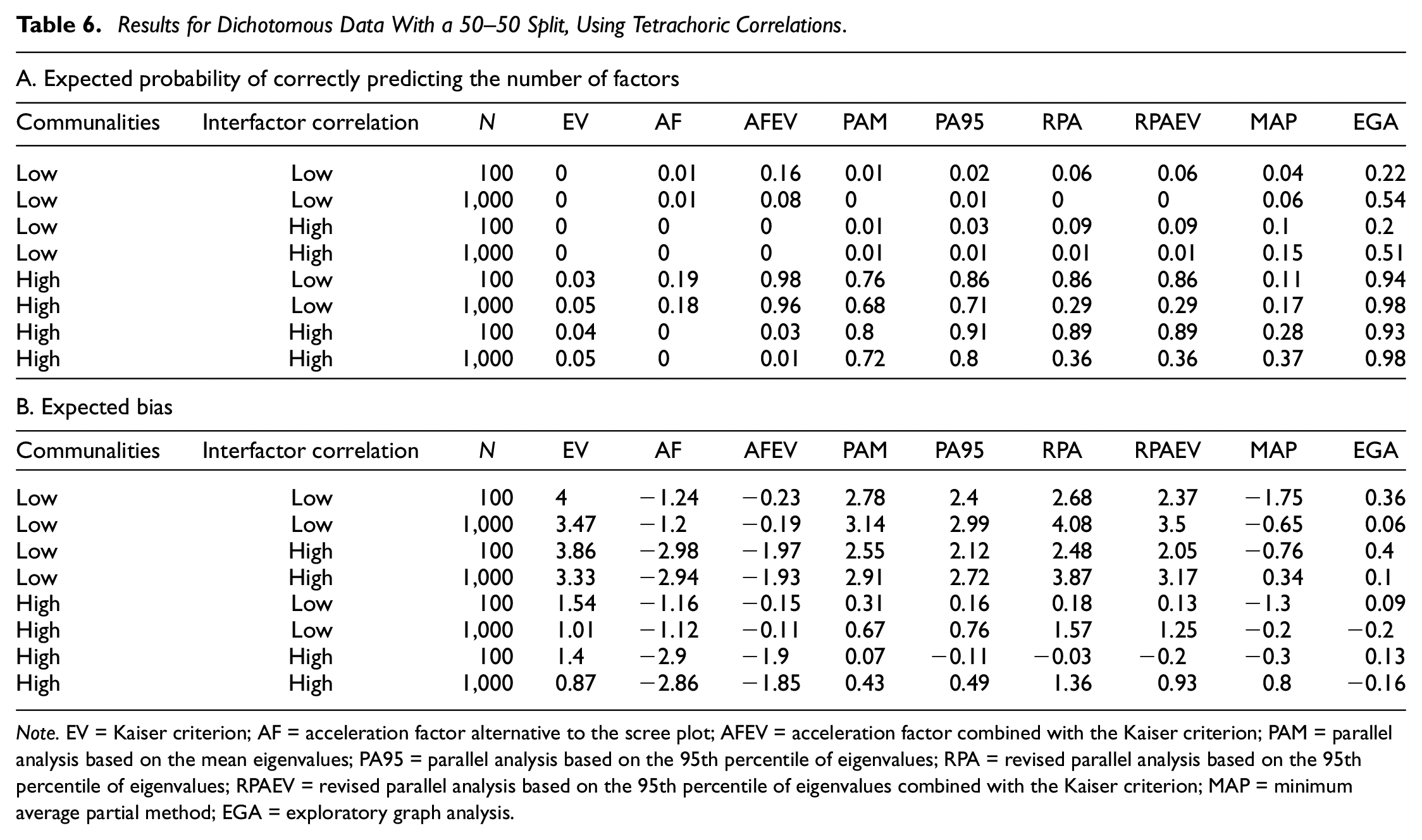
Both Figures 3 and 4 and their corresponding Tables 5 and 6 show the results for dichotomous data with a 50–50 split between zeroes and ones. The difference being that the latter displays the outcomes for the analysis using tetrachoric correlations, and the former using Pearson correlations.
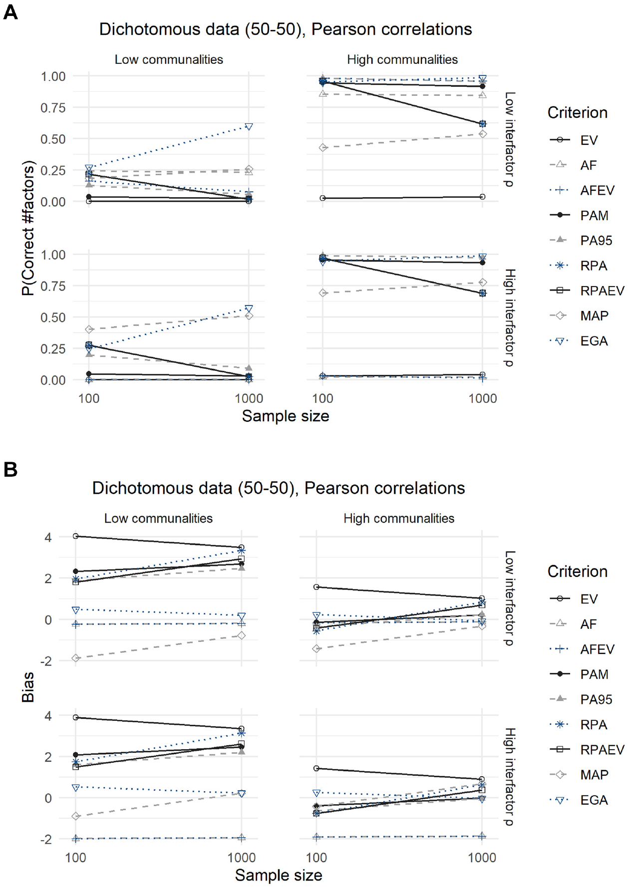
Results for Dichotomous Data With a 50–50 Split, Using Pearson Correlations: (A) Expected Probability of Correctly Predicting the Number of Factors and (B) Expected Bias.
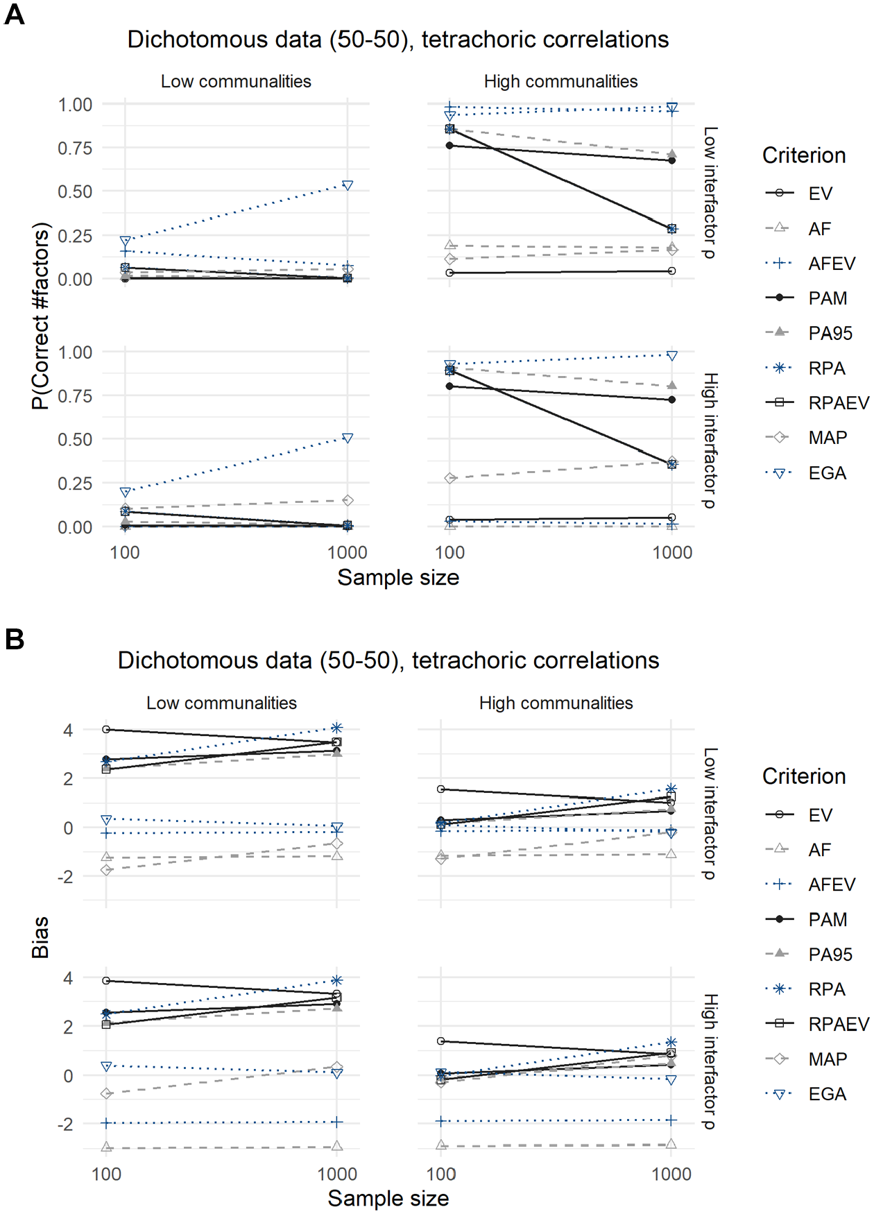
Results for Dichotomous Data With a 50–50 Split, Using Tetrachoric Correlations: (A) Expected Probability of Correctly Predicting the Number of Factors and (B) Expected Bias.
Results for Continuous Data With a 50–50 Split, Using Pearson Correlations.
Results for Dichotomous Data With a 50–50 Split, Using Tetrachoric Correlations.
Note. EV = Kaiser criterion; AF = acceleration factor alternative to the scree plot; AFEV = acceleration factor combined with the Kaiser criterion; PAM = parallel analysis based on the mean eigenvalues; PA95 = parallel analysis based on the 95th percentile of eigenvalues; RPA = revised parallel analysis based on the 95th percentile of eigenvalues; RPAEV = revised parallel analysis based on the 95th percentile of eigenvalues combined with the Kaiser criterion; MAP = minimum average partial method; EGA = exploratory graph analysis.
Using Pearson correlations, the expected probabilities of accurately predicting the number of factors are nearly identical to those obtained from the analysis of continuous data. One exception is the MAP criterion, which now performs significantly better in almost every scenario and even outperforms the EGA method when faced with small samples, low communalities from major factors and high interfactor correlations. In this case its expected accuracy rises to 0.4 compared with 0.25 for EGA. Looking at the second panel of Figure 3, the differences are again minimal. The expected biases of the EV criterion rise and those of PA95 and RPA decrease slightly. Only the MAP criterion becomes significantly less biased.
Results change when we analyze the data using tetrachoric correlations (Figure 4 and Table 6). More specifically, the expected accuracies of all criteria shift downward but the relative performances remain similar to the continuous case. Remarkably, the MAP criterion loses its edge over the other criteria when using tetrachoric correlations. In terms of expected bias, conclusions are very similar to those drawn earlier when analyzing continuous data. However, the expected bias of the MAP criterion has shifted further downward in comparison the case of binary data and an analysis with Pearson correlations. It, however, still outperforms the case of continuous data.
Dichotomous Data (75–25 Split)
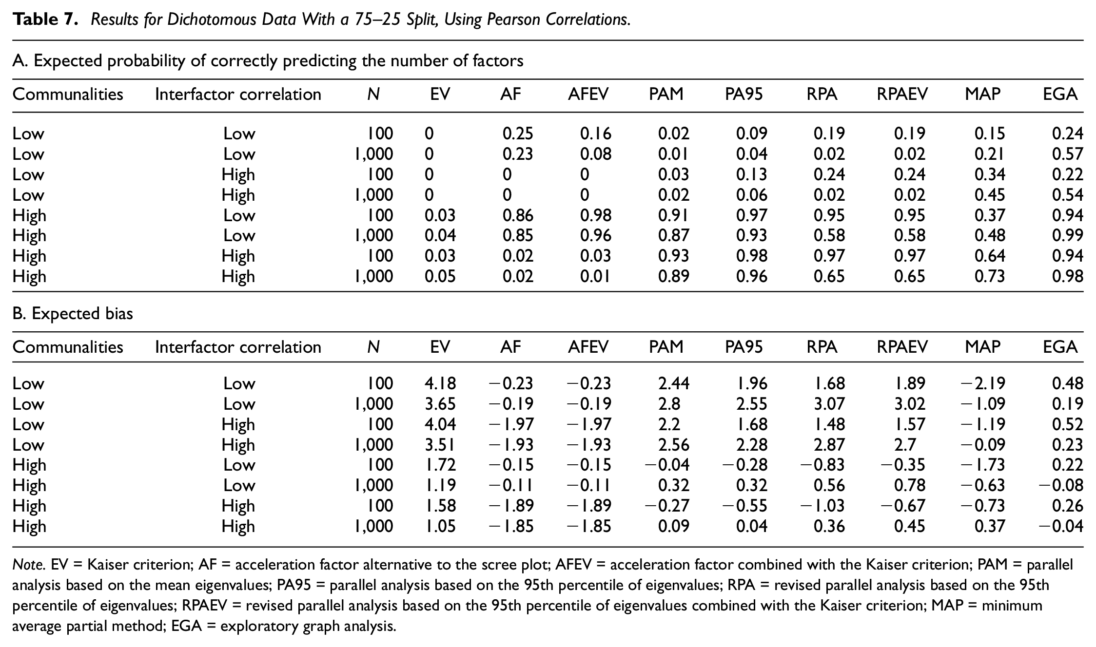
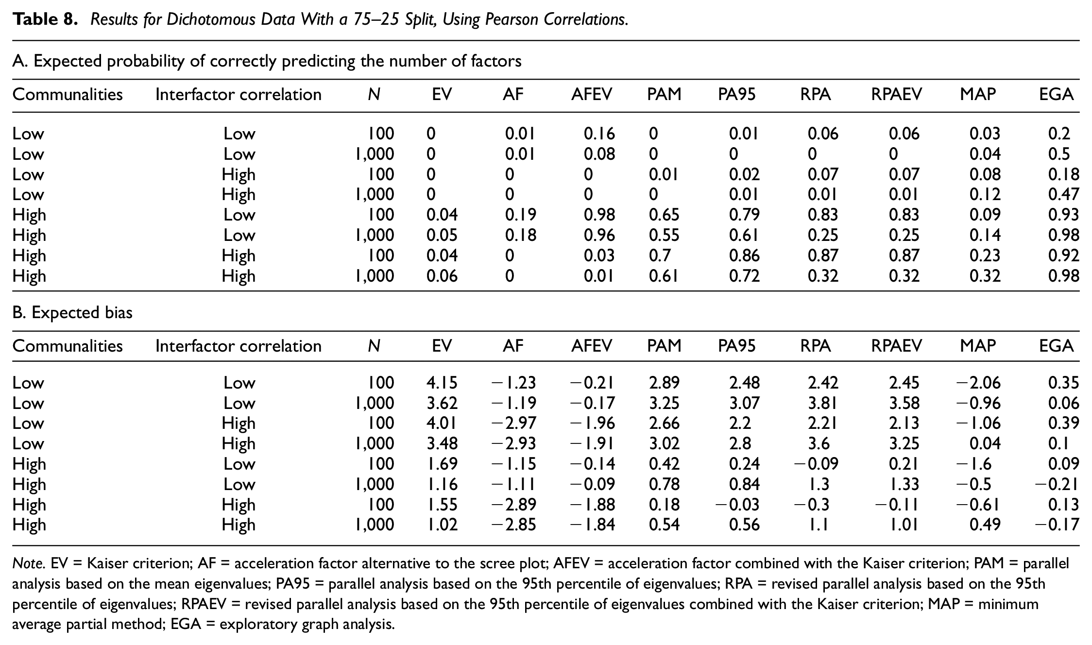
Compared with the analyses of the dichotomous data with a 50–50 split, conclusions are identical for the dichotomous data with a 75–25 split between zeroes and ones, as displayed in Figures 5 and 6 and their corresponding Tables 7 and 8.
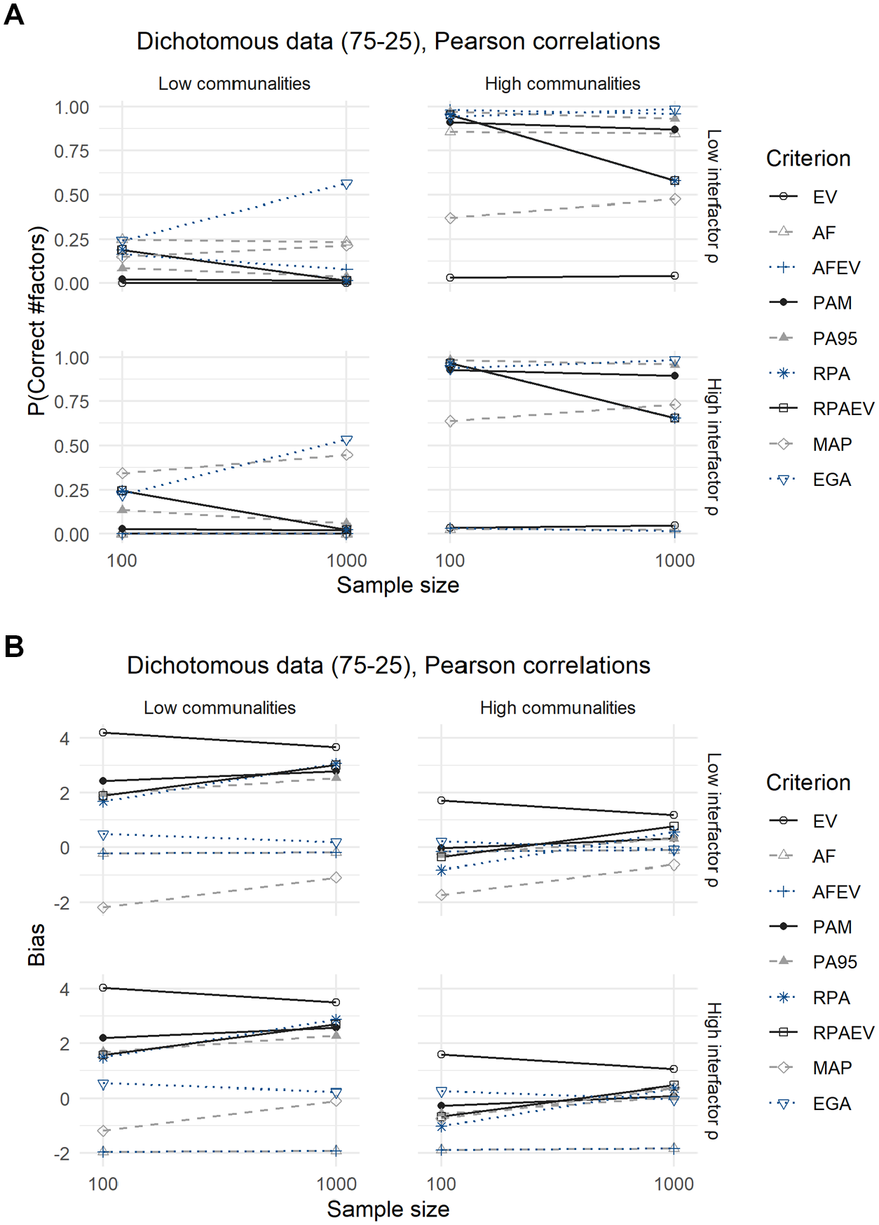
Results for Dichotomous Data With a 75–25 Split, Using Pearson Correlations: (A) Expected Probability of Correctly Predicting the Number of Factors and (B) Expected Bias.
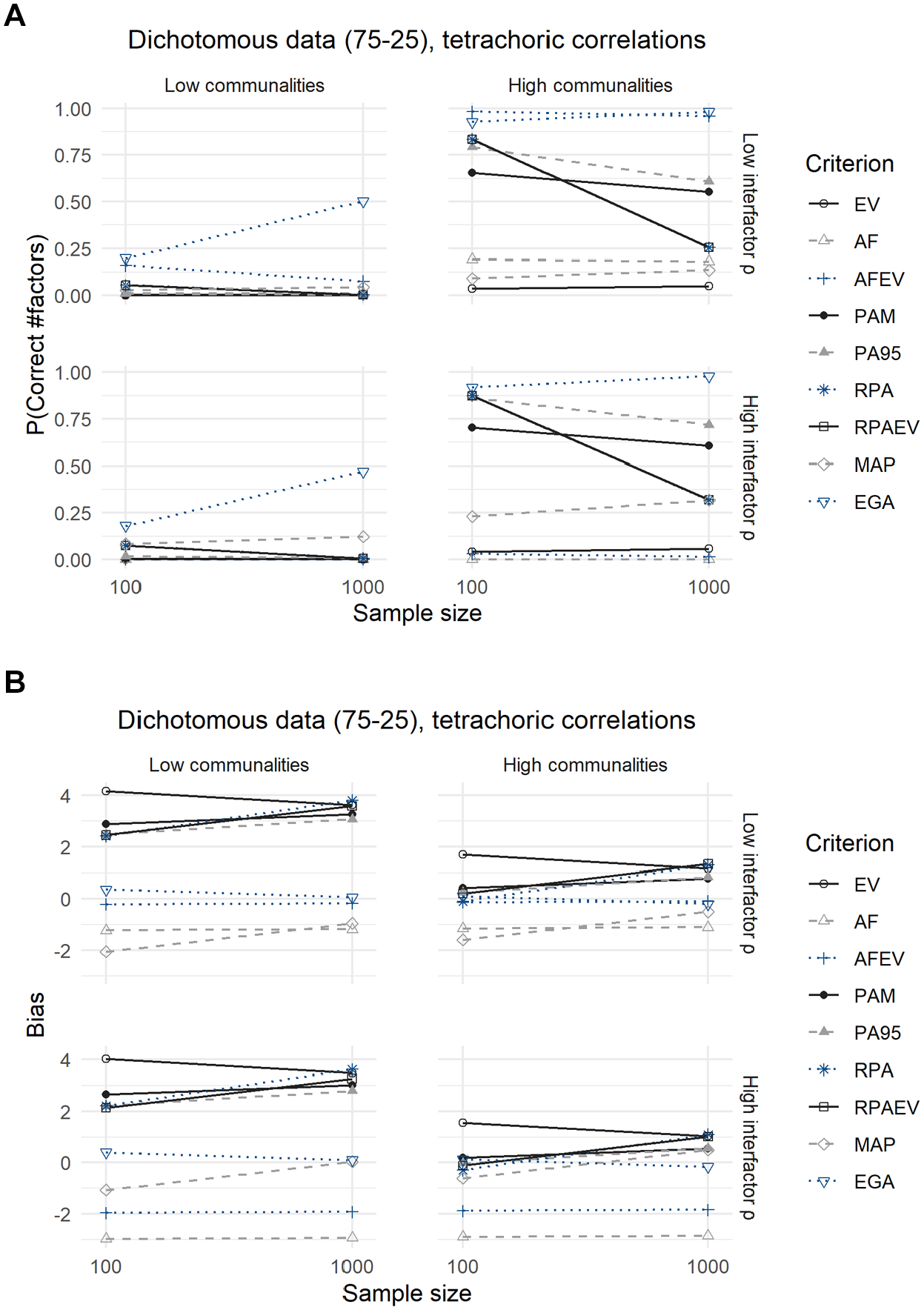
Results for Dichotomous Data With a 75–25 Split, Using Tetrachoric Correlations: (A) Expected Probability of Correctly Predicting the Number of Factors and (B) Expected Bias.
Results for Dichotomous Data With a 75–25 Split, Using Pearson Correlations.
Note. EV = Kaiser criterion; AF = acceleration factor alternative to the scree plot; AFEV = acceleration factor combined with the Kaiser criterion; PAM = parallel analysis based on the mean eigenvalues; PA95 = parallel analysis based on the 95th percentile of eigenvalues; RPA = revised parallel analysis based on the 95th percentile of eigenvalues; RPAEV = revised parallel analysis based on the 95th percentile of eigenvalues combined with the Kaiser criterion; MAP = minimum average partial method; EGA = exploratory graph analysis.
The MAP criterion performs significantly better when using Pearson correlations in terms of both the expected probability of predicting the correct number of factors to retain as well as the expected bias, but loses this advantage when employing tetrachoric correlations. In addition, using tetrachoric correlations leads to a decrease in the expected accuracies of all criteria, but relative performances remain the same. The underperformance of the MAP criterion is again due to its tendency to underextract in this case.
Discussion
While many criteria have been developed to aid the choice of the number of factors to retain, we show that the most popular ones, such as the Kaiser criterion and scree plot, underperform. Studies by both Yang and Xia (2015) and Ruscio and Roche (2012) come to the same conclusions regarding the performance of the Kaiser criterion. We do, however, notice a better performance of the scree plot in the presence of high communalities from major factors and low interfactor correlations.
Both parallel analysis based on the mean eigenvalue and on the 95th percentile perform well in situations with high communalities from major factors. Research by Auerswald and Moshagen (2019), Cho et al. (2009), Crawford et al. (2010), Golino, Shi, et al. (2020) and Ruscio and Roche (2012) also support these conclusions. Yet, none of these studies point to the severe underperformance of parallel analysis when variables are only weakly influenced by their common factors. Only in small samples can revised parallel analysis (Green et al., 2012) alleviate some of the concerns regarding the accuracy of traditional parallel analysis. The study by Green et al. (2016) that indicates the preference of this former method in almost all circumstances can therefore not be endorsed. Auerswald and Moshagen (2019) already found this result for revised parallel analysis based on the reduced correlation matrix, and our results confirm it for the variant based on the full correlation matrix. In addition, revised parallel analysis shows accuracies that decrease as sample size increases. In general, however, larger sample sizes increase the accuracy of the criteria considered, which is in line with results obtained by Li et al. (2020).
EGA performs at least equally well as the criteria considered, yet usually outperforms them. While Golino, Shi, et al. (2020) also find that this criterion can match the performance of traditional parallel analysis, our results favor the former even more: Even in circumstances where most other criteria fail, is EGA able to achieve reasonable accuracy with larger sample sizes. 1 Only in the case of binary data and analysis with Pearson correlations, can the minimum average partial method outperform EGA when faced with small samples and low communalities from major factors.
While tetrachoric correlations are usually recommended because they produce unbiased estimates of the relationships among the latent underlying continuous variables (Kirk, 1973; Olsson, 1979), we find that the use of tetrachoric correlations worsens the performance of all criteria when applied to binary data. Yet, the relative performances remain identical to the continuous case. Determining the number of factors to retain is therefore preferably done using the Pearson correlation matrix. It is important to note that the preference for Pearson correlations only applies to the determination of the optimal number of factors to retain, not to the rest of the factor analytic process. Studies (e.g., Barendse et al., 2015; Kaltenhauser & Lee, 1976; Lee et al., 2012) have shown that when extracting loadings, polychoric correlations are still preferred when working with ordinal data. In case of binary data, tetrachoric correlations are therefore still recommended when estimating loadings. In addition, this result was not previously discussed by other factor retention simulation studies, given that most of these studies apply tetrachoric correlations directly and do not compare it with the performances under Pearson correlations (see Table 1). Only Cho et al. (2009) find a similar conclusion when studying the accuracy of parallel analysis and reason that this results from the fact that tetrachoric correlations tend to be higher. This causes the eigenvalues of these correlation matrices to be higher for the first components and smaller for the subsequent ones. Finally, we find that the split between zeroes and ones does not affect the accuracy of the factor retention criteria for binary data.
Conclusion and Directions for Future Research
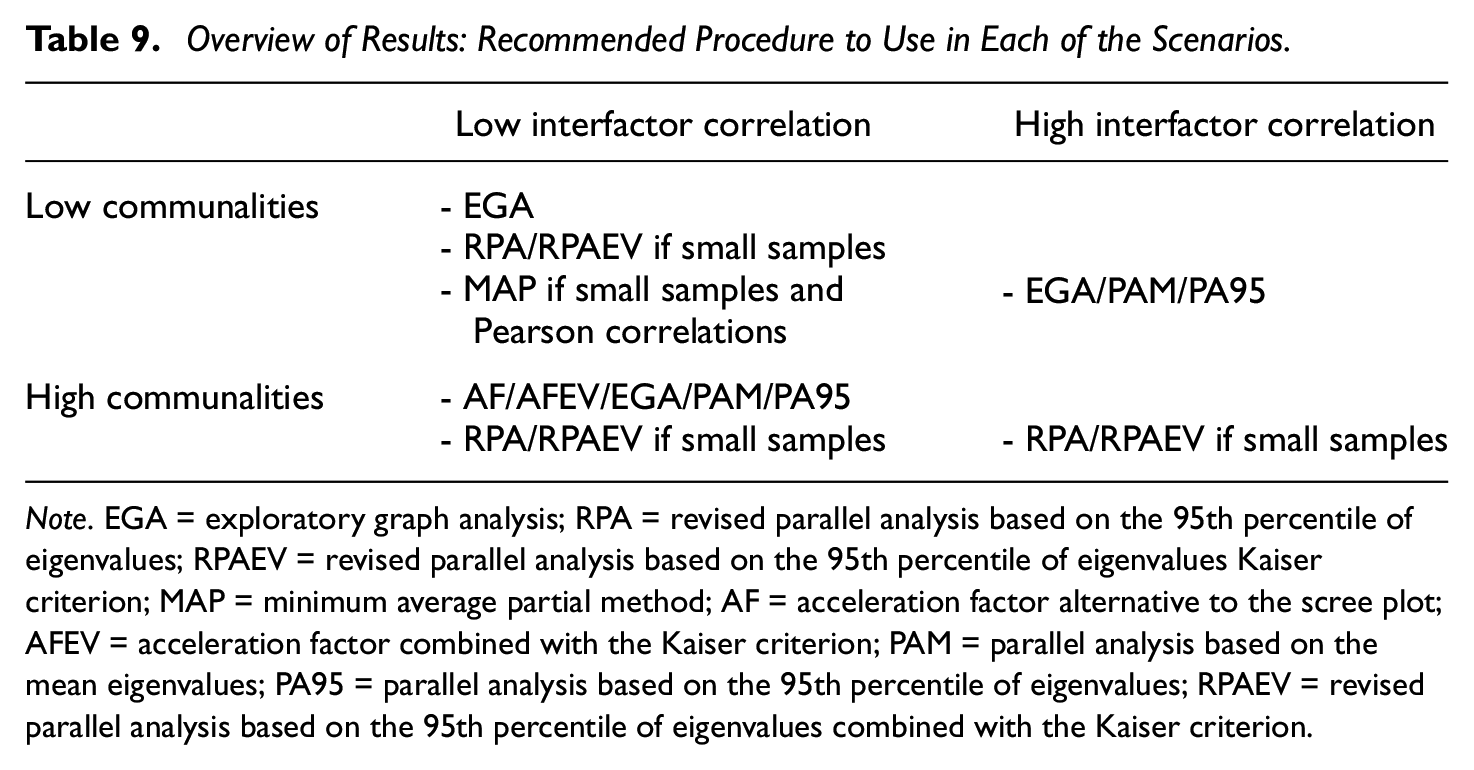
The simulation results give way to several recommendations for researchers (cf. Table 9). First, when working with continuous data, EGA would seem the preferred criterion in all circumstances. In addition, researchers less familiar with this technique or its implementation might rely on revised parallel analysis (with or without the added use of the Kaiser criterion) in small samples. If the researcher is confident about the construction of his or her factors in that the manifest variables are all highly related to their accompanying latent variable in addition to disposing of a large sample, traditional parallel analysis (either based on mean or the 95th percentile of the eigenvalues) is also a good option. 2
Overview of Results: Recommended Procedure to Use in Each of the Scenarios.
Note. EGA = exploratory graph analysis; RPA = revised parallel analysis based on the 95th percentile of eigenvalues; RPAEV = revised parallel analysis based on the 95th percentile of eigenvalues Kaiser criterion; MAP = minimum average partial method; AF = acceleration factor alternative to the scree plot; AFEV = acceleration factor combined with the Kaiser criterion; PAM = parallel analysis based on the mean eigenvalues; PA95 = parallel analysis based on the 95th percentile of eigenvalues; RPAEV = revised parallel analysis based on the 95th percentile of eigenvalues combined with the Kaiser criterion.
Dichotomous data, either with a 50–50 or 75–25 split between zeroes and ones, can additionally benefit from the use of the minimum average partial method if analyzed with Pearson correlations. The MAP can be a valid, but less effective, alternative to the EGA method in case the researcher is more familiar with the former. Yet, this criterion loses its edge when analyzing dichotomous data with tetrachoric correlations. In addition, the use of this kind of correlation lowers the performance of all criteria.
But even when adhering to these guidelines, the number of factors extracted might not be correct. Underextraction compresses variables into a smaller factor space which leads to loss of information, neglect of important factors, distorted results, and increased error in the loadings. On the contrary, overextraction diffuses variables across a larger space, resulting in splitting of factors (Auerswald & Moshagen, 2019; Hayton et al., 2004). Underextraction is therefore a bigger problem and must be avoided at all costs. When multiple criteria give different answers, it is hence safer to choose the largest estimate of the optimal number of factors.
Overall, these results unveil opportunities for applied researchers: While Dolnicar et al. (2011) show that a binary response format saves respondent time and is perceived simpler while not influencing reliability or interpretations of results, our results show that at least part of the EFA process can be executed without loss of accuracy.
Yet, the focus on binary data has the inherent limitation to be only of moderate use in practice as Likert-type scales are still more often employed. Whether such data are suited for analysis using traditional factor retention criteria is still debated (Holgado-Tello et al., 2010) and therefore worth further investigation.
The data simulation procedure employed (Hong, 1999; Tucker et al., 1969) is considered standard in EFA research, yet also has its limitations. Most noticeably the fact that the sampled data follow a multivariate normal distribution. Auerswald and Moshagen (2019), however, show this does not influence the accuracy of these criteria in case of continuous data.
In addition, we have kept the degree of overdetermination constant, yet previous research has pointed to interplay between this degree and the sample size (e.g., Gaskin & Happell, 2014). Conclusions drawn regarding the latter should therefore be viewed in the context of our study. Repeating the same study, but varying the number of factors and variables per factor, is therefore another possibly fruitful avenue for future research. Other fixed 3 characteristics of the simulation design, such as the number of minor factors, common ratio, and correlations between major and minor factors, were all kept constant, following other authors. Yet, future research would benefit from also assessing the impact of these variables on the performance of factor analysis.
The criteria and methods studied were largely based on an overview of current academic research, yet many more exist. Further research would profit from considering more, maybe less well-known procedures.
A last recommendation is the execution of a simulation study that takes into account more complex factor structures, given that this study only examines data with a loading matrix that satisfies perfect simple structure. Auerswald and Moshagen (2019) argue that cross-loadings should have a beneficial effect on both accuracy and bias because they increase the explained variance, yet Li et al. (2020) find the opposite. These last authors regard cross-loadings as a form of modeling error, as these are loadings on “minor factors.” We have also included “minor factors,” yet not by modeling cross-loadings on major factors. This could explain why the accuracies we obtain are lower than those found by Auerswald and Moshagen (2019). Yet, these scenarios remain a recommendation for future research.
Supplemental Material
sj-pdf-1-epm-10.1177_00131644211059089 – Supplemental material for Exploratory Graph Analysis for Factor Retention: Simulation Results for Continuous and Binary Data
Supplemental material, sj-pdf-1-epm-10.1177_00131644211059089 for Exploratory Graph Analysis for Factor Retention: Simulation Results for Continuous and Binary Data by Tim Cosemans, Yves Rosseel and Sarah Gelper in Educational and Psychological Measurement
Footnotes
Declaration of Conflicting Interests
The authors declared no potential conflicts of interest with respect to the research, authorship, and/or publication of this article.
Funding
The authors received no financial support for the research, authorship, and/or publication of this article.
Supplemental Material
Supplemental material for this article is available online.
Notes
References
Supplementary Material
Please find the following supplemental material available below.
For Open Access articles published under a Creative Commons License, all supplemental material carries the same license as the article it is associated with.
For non-Open Access articles published, all supplemental material carries a non-exclusive license, and permission requests for re-use of supplemental material or any part of supplemental material shall be sent directly to the copyright owner as specified in the copyright notice associated with the article.