
Abstract
Background:
The mean population mood has been demonstrated to strongly correlate with the prevalence of depression in European populations. Mean population mood has, therefore, been proposed as both a metric to measure the impact of population-level interventions to prevent depression and a target for public health policy.
Aim:
To demonstrate the relationship between mean population mood and the prevalence of depression using Australian data in order to broaden the applicability of this finding to the Australian population.
Methods:
We used data from the Geelong Osteoporosis Study to assess the relationship between population mean mood and depression. Participants reported mood symptoms via questionnaire (the Hospital Anxiety and Depression Scale or General Health Questionnaire-12). Depression was diagnosed by semi-structured clinical interview (Structured Clinical Interview for Diagnostic and Statistical Manual of Mental Disorders, Fourth Edition, Non-patient Edition). Stratification by age and socio-economic status was used to create subpopulation groups. Socio-economic status was measured using Index of Relative Socio-economic Advantage and Disadvantage quintiles, an area-based measure based on Australian census data and published by the Australian Bureau of Statistics. The mean subpopulation questionnaire scores and subpopulation prevalence of depression were then analysed using regression and predictive models.
Results:
Mean subpopulation questionnaire scores correlated well with the prevalence of depression across socio-economic status groups in women but not age groups. Questionnaire scores tended to underestimate the prevalence of depression in the young and overestimate it in the elderly.
Conclusion:
The mean population mood was demonstrated to correlate with the population prevalence of depression in Australia for women, but not for men. Due to the issues of questionnaire validity and sample size in the oldest age groups, the age analysis is unlikely to be a representative of population characteristics. Further work to identify population determinants of mean mood could potentially create policy targets to reduce the prevalence of depression.
Introduction and background
Depression is a disabling illness and has been described as producing a greater decrement in health than chronic disease such as angina, arthritis and asthma (Moussavi et al., 2007). The most recent National Survey of Mental Health and Wellbeing found 1 in 20 Australians had experienced a depressive episode in the last 12 months (Australian Bureau of Statistics, 2008). The prognosis of spontaneous recovery is poor after multiple episodes, with frequent remission and relapses (Solomon et al., 2000). In children and adolescents, depression is associated with impaired academic performance, poorer social function and a 30 times greater risk of completed suicide (Horowitz and Garber, 2006); in adults, depression is an important comorbidity for physical illness, is associated with high levels of psychological distress and carries an increased mortality even for subclinical depressive symptoms (Department of Health and Ageing, 2013b; Frasure-Smith et al., 1993b). In Australia, 4.1% of the population suffered a depressive episode in the previous year (Australian Bureau of Statistics, 2008), and depression and anxiety are together the leading cause of disease burden for women and the second highest cause for men (Begg et al., 2007). The latest Australian Burden of Disease statistics reveal that for those under the age of 50 years, mental disorders account for the leading cause of life lost to premature death or living with illness (Australian Institute of Health and Welfare, 2016).
It is often said that prevention is better than cure, and this is applicable to depression. It is estimated that even with optimal care, less than 35% of the disease burden can be averted (Andrews et al., 2004). The prevalence of depression remained relatively unchanged between the 1997 and 2007 National Survey of Mental Health and Wellbeing (Department of Health and Ageing, 2008, 2013b). A recent literature review found that this can partly be explained by increasing public awareness of disease symptomatology but cannot be explained by changes in risk factor exposure such as natural disasters (Jorm et al., 2017). Public health policies such as the Access to Allied Psychological Services 2002; Better Access Scheme to Psychiatrists, Psychologists and General Practitioners through the Medicare Benefits Schedule 2006; and beyondblue have almost doubled access to mental health-care services and reduced public stigma (Department of Health and Ageing, 2013a) but have yet to show an effect on the epidemiology of depression (Jorm et al., 2017). It has been argued that this is in part due to a focus on treatment of established disease without corresponding efforts on prevention (Jorm, 2014). Of concern for the former approach, only 41% of Australians with mental illness on active treatment were reported to have received a minimally adequate treatment, a figure representing only 16% of all persons with a mental illness (Harris et al., 2015).
The basis of preventive medicine is that interventions can be targeted at risk factors in order to reduce the incidence of disease. For continuous risk factors such as blood pressure or body mass index (BMI), the decision to treat requires a binary distinction to be made at a defined threshold between health and disease. The label of being hypertensive or obese indicates that one has deviated from the population norm a sufficient amount for their state to be considered pathological. The corollary of this is the implication that individuals with risk factor profiles within normal limits are healthy and do not require treatment. This assumption was challenged by the eminent epidemiologist Geoffrey Rose in his seminal paper (Rose and Day, 1990). Rose was able to show that for conditions such as hypertension, the entire population blood pressure distribution shifted in populations with a high prevalence of hypertension and that the population mean predicted the prevalence of diseased ‘deviants’ (see Figure 1). The population risk of hypertension did not suddenly change at the treatment threshold; rather, risk increased at all levels of mean blood pressure. Rose argued that this diseased tail of the population distribution is merely a subset of its parent population distribution and that successful prevention could be achieved by interventions that impact whole populations rather than only those at highest risk.
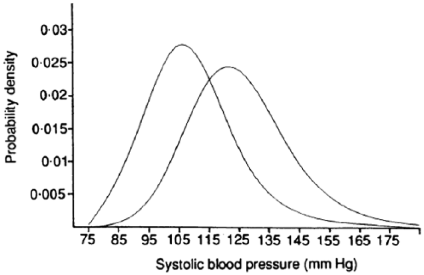
Distribution of systolic blood pressures for the averages of the highest and lowest mean blood pressures from the Intersalt study.
Rose speculated that clinical depression shared a similar relationship with the population mood distribution but lacked the data to demonstrate this. Almost two decades later, Veerman et al. (2009) used data from a major European study to test Rose’s argument. Using data from the European Outcome in Depression International Network study, they showed that populations with higher levels of depression exhibited lower mean moods, as measured by Beck Depression Inventory (BDI) score. Furthermore, the population mean mood was also able to accurately predict the prevalence of depression robustly across five different countries and in multiple subpopulations within those countries. Subsequent studies have demonstrated a relationship between the population mean and case frequency in paediatric mental health as well as adolescent gambling (Goodman and Goodman, 2011; Hansen and Rossow, 2012).
In this study, we attempt to replicate the work of Veerman et al. (2009) in an Australian context. If the mean population mood predicts the prevalence of depression, it follows that policies that can alter the population mean mood may alter the prevalence of depression as well. To date, no primary prevention mental health policies (Australian or otherwise) have targeted the population mean mood as an explicit goal. Our work helps explain why policies involving the entire population (including mentally well individuals) are useful in reducing the prevalence of depression and complement existing policies targeting already depressed individuals. This would be analogous to promoting diet and exercise to individuals while taxing junk food to reduce the prevalence of obesity on a population level. Our paper also provides evidence for the use of the population mean mood as a potential metric for evaluating interventions aimed at depression. Although further research would be needed to validate this, population mean mood may be more sensitive to changes across the entire mood spectrum and not merely those who are severely depressed or above a questionnaire specific threshold.
Methods
Participants
The Geelong Osteoporosis Study (GOS) is a large, ongoing, population-based study located in south-eastern Australia. Originally, age-stratified samples of 1494 women (aged 20–94 years, response rate 77.1%) and 1540 men (aged 20–93 years, response rate 67.0%) were recruited at random from the electoral rolls for the Barwon Statistical Division between 1994–1997 and 2001–2006, respectively, and have returned for ongoing assessment. A further sample of 246 women listed as aged 20-29 years on the 2005 electoral roll were recruited in 2006-2008. Further details of the study have been published elsewhere (Pasco et al., 2012).
For this study, data were used from the GOS 10- and 15-year follow-up for women and GOS 5-year follow-up of men. Of 1127 women who participated in the GOS 10-year follow-up and 849 women who participated in the GOS 15-year follow-up, participants for whom complete psychiatric data were not available were excluded from the current analyses, resulting in samples of 1059 and 787, respectively. For men, of the 978 who participated in the 5-year follow-up, participants for whom psychiatric data were not available were also excluded, resulting in a sample of 911. The Human Research Ethics Committees at Barwon Health, Deakin University and University of Queensland approved the study. All participants provided informed, written consent.
Data
Depression was determined using both clinical interviews and screening questionnaires at various GOS follow-up assessments (see Table 1).
Mental health assessment in the Geelong Osteoporosis Study.
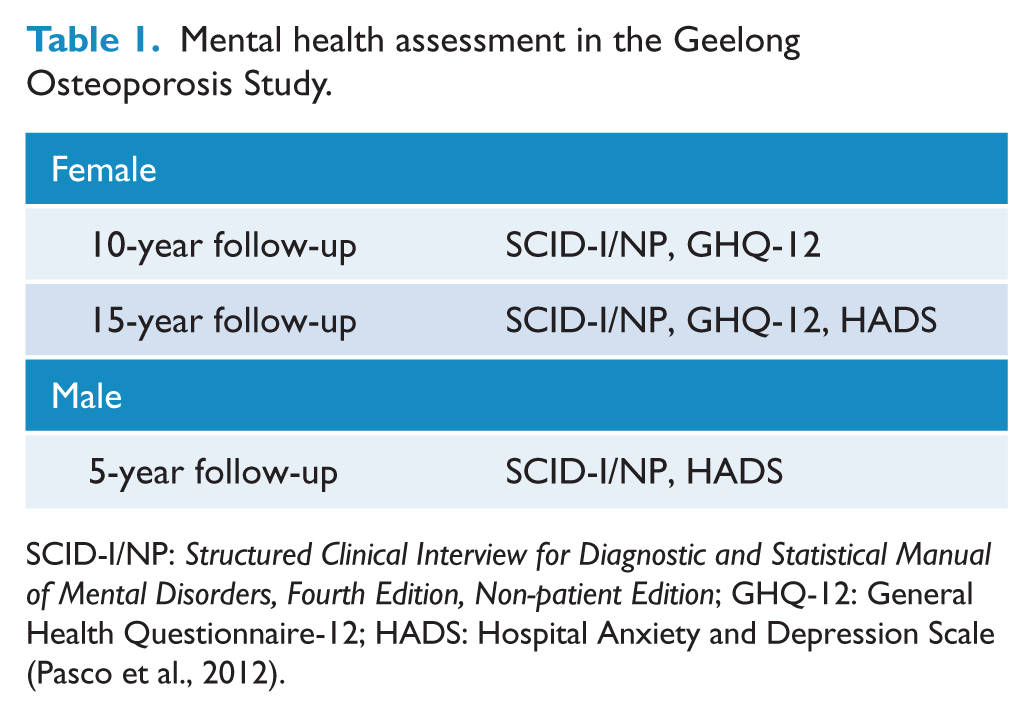
SCID-I/NP: Structured Clinical Interview for Diagnostic and Statistical Manual of Mental Disorders, Fourth Edition, Non-patient Edition; GHQ-12: General Health Questionnaire-12; HADS: Hospital Anxiety and Depression Scale (Pasco et al., 2012).
The Structured Clinical Interview for Diagnostic and Statistical Manual of Mental Disorders, Fourth Edition, Non-patient Edition (SCID-I/NP) was used to identify current diagnoses of depression including major depressive disorder (MDD), minor depression, bipolar disorder, dysthymia, mood disorder due to a general medical condition and/or substance-induced mood disorders (First et al., 2002). The definition ‘clinical depression’ was used in this study and included those meeting criteria for current MDD and dysthymia. All interviews were conducted by personnel with postgraduate qualifications in psychology who were trained using live and videotaped interviews under the supervision of a psychiatrist.
The Hospital Anxiety and Depression Scale (HADS) is a self-administered questionnaire consisting of 14 four-point Likert-scale items, 7 for anxiety (HADS-A subscale) and 7 for depression (HADS-D subscale), encompassing the past week. The HADS is a widely used instrument designed to assess both caseness and symptomatology of depression and anxiety in epidemiological research and specialist care and has been shown to have good specificity and sensitivity in both hospitalised and general populations (Bjelland et al., 2002; Zigmond and Snaith, 1983).
The General Health Questionnaire-12 (GHQ-12) contains 12 items scored from 0 to 3: 6 pertaining to positive mood and 6 to negative mood and has similarly been validated in the general population (Craig, 2006; Donath, 2001). The HADS and GHQ-12 have comparable sensitivity and specificity, and both have been used in other Australian studies (Boyes et al., 2013; Donath, 2001; Love et al., 2004).
SES was categorised into quintiles based on Index of Relative Socio-economic Advantage and Disadvantage (IRSAD) score. The IRSAD quintiles range from 1 to 5, with 1 being the most disadvantaged and 5 being the most advantaged. The IRSAD provides a relative measure of SES at the area level and is a composite measure that includes level of income, employment status (employed vs unemployed) and type of occupation ranging from unskilled employment to professional positions. The IRSAD score is one of the Socio-economic Indexes for Areas (SEIFA) indices published by the Australian Bureau of Statistics and has been previously validated by academic and policy research experts including peer review of input variables (Pink, 2013). The IRSAD data for the 5-year male follow-up and 10-year female follow-up were derived from the 2006 Australian census and the 15-year female follow-up from the 2011 Australian census. Participants were categorised into quintiles according to cut-off points of the Barwon Statistical Division determined by 2006 Australian Census Data (Brennan et al., 2013).
Analysis
Given that the distribution of mental disorders in the Australian population differs by age group and socio-economic status (SES; Australian Institute of Health and Welfare, 2016), we aimed to correlate the mean GHQ-12 and HADS scores for subpopulation groups with the subpopulation prevalence of clinical depression. Subpopulations were generated according to age and SES. Age groups used were <40, 41–60, 61–80 and >80 years and SES groups by IRSAD quintiles.
The relationship between mean subpopulation questionnaire score and prevalence of clinical depression was established according to the methodology employed by Veerman et al. (2009). First, a simple linear relationship between subpopulation questionnaire means and prevalence of clinical depression was calculated for both questionnaires. Second, we constructed a model that described the distribution of HADS or GHQ-12 scores for different follow-up years. We assumed participants could be diagnosed with depression based on their questionnaire responses and calculated a questionnaire threshold that best corresponded to the prevalence of clinical depression. The model gave two estimates of subpopulation depression prevalence: the proportion of the modelled distribution above the threshold (‘distribution prevalence’) and the proportion of real participants whose questionnaires were above the threshold value (‘questionnaire prevalence’).
Modelling
We modelled frequency distributions of GHQ-12 and HADS scores by age (<40, 41–60, 61–80 and >80 years) and SES for all possible questionnaire scores to a mathematical distribution. Low questionnaire scores are more common than high values. Therefore, we tested Weibull, beta and gamma models, as each describe skewed distributions. We used the least squares method embedded in the ‘Solver’ add-in function of Microsoft Excel 2010 for our analysis. Modelling is described in detail in Supplementary Appendix 1.
Sensitivity analysis
One interpretation of a correlation between depression and questionnaire scores is that depressed individuals ‘pull up’ the mean by virtue of their high questionnaire responses. As a result, a population with a high prevalence of depression will exhibit a higher mean questionnaire score compared to a population with a low prevalence. Additionally, depressed individuals may differ in their follow-up participation from non-depressed individuals. In order to mitigate these effects, we analysed the relationship between the mean questionnaire score and clinical depression before and after the HADS or GHQ-12 responses of depressed individuals were removed.
Results
Mean questionnaire scores and proportion meeting criteria for clinical depression according to age and SES for the different subpopulations are summarised in Table 2. The complete data analysis results can be found in Supplementary Appendices 2–5. IRSAD quintiles 1 and 2 (most disadvantaged) collectively represent 35.7% of our sample, and IRSAD quintiles 4 and 5 (most advantaged) represented 44.9% of our sample (Brennan et al., 2013).
Mean questionnaire scores and proportion meeting criteria for depression according to age and SES for men and women.
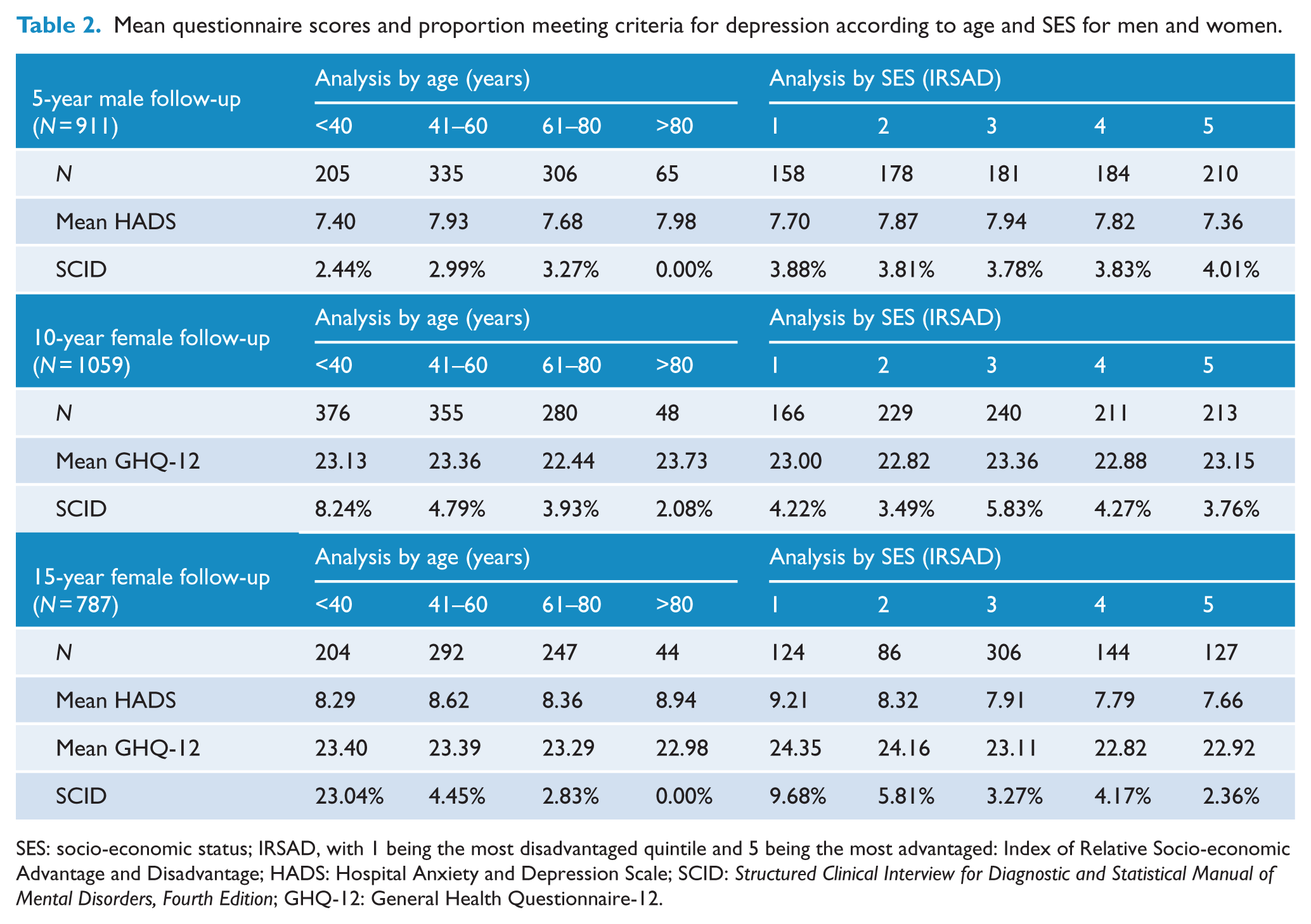
SES: socio-economic status; IRSAD, with 1 being the most disadvantaged quintile and 5 being the most advantaged: Index of Relative Socio-economic Advantage and Disadvantage; HADS: Hospital Anxiety and Depression Scale; SCID: Structured Clinical Interview for Diagnostic and Statistical Manual of Mental Disorders, Fourth Edition; GHQ-12: General Health Questionnaire-12.
HADS analysis by age
Of the 911 men and 787 women who completed the HADS, 27 (2.96%) men and 72 (9.15%) women were classified as meeting criteria for clinical depression. There was no relationship between mean age group HADS scores and clinical depression (R2 = 0.00; see Figure 2). HADS scores tended to overestimate depression in the >80 years age groups and underestimate it in the <40 years age groups. A markedly high proportion of women aged <40 years met criteria for clinical depression (23.04%), comprising mostly of dysthymia (36 cases) rather than MDD (12 cases). The prevalence predictions generated by the beta, gamma and Weibull distribution ranged from modest to poor (R2 range 0.00–0.38), with the best predictions generated by the beta distribution using the questionnaire cut-off method (see Table 3).
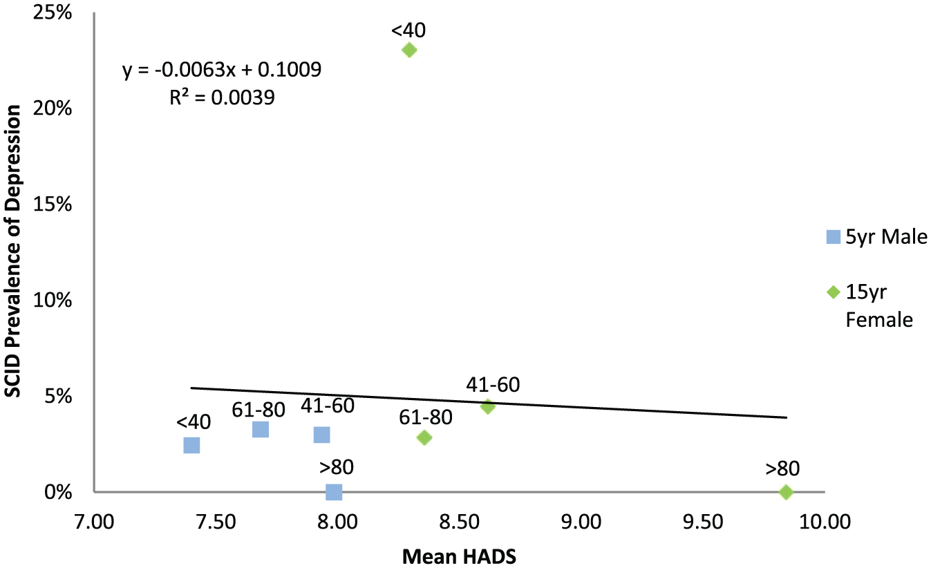
Regression between depression and mean questionnaire scores for different age groups (years) for men and women.
Evaluation of agreement between the prevalence of interview-diagnosed depression and prevalence predictions by mean questionnaire score using linear regression and beta, gamma and Weibull distributions.
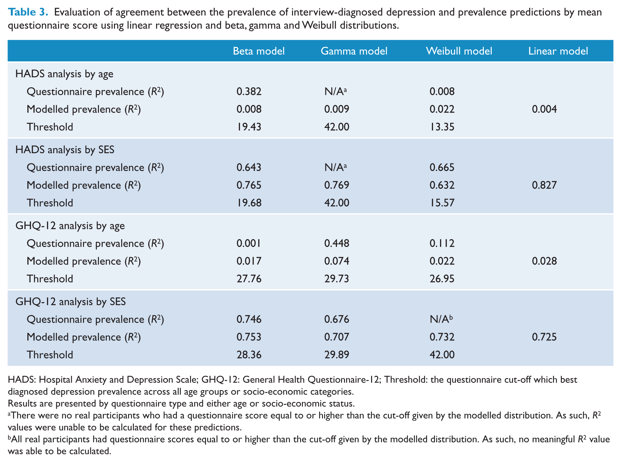
HADS: Hospital Anxiety and Depression Scale; GHQ-12: General Health Questionnaire-12; Threshold: the questionnaire cut-off which best diagnosed depression prevalence across all age groups or socio-economic categories.
Results are presented by questionnaire type and either age or socio-economic status.
There were no real participants who had a questionnaire score equal to or higher than the cut-off given by the modelled distribution. As such, R2 values were unable to be calculated for these predictions.
All real participants had questionnaire scores equal to or higher than the cut-off given by the modelled distribution. As such, no meaningful R2 value was able to be calculated.
GHQ-12 analysis by age
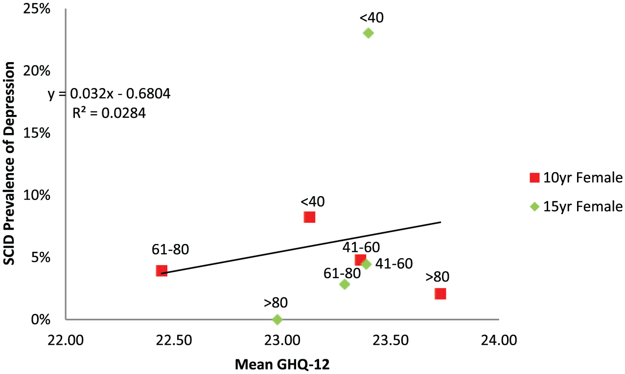
Of the 1846 women who completed the GHQ-12, 137 (7.42%) women met the criteria for clinical depression. There was a weak relationship between mean age group GHQ-12 score and clinical depression (R2 = 0.03; see Figure 3). Similar to the HADS analysis, the >80 age group contained fewer participants than the other groups, and GHQ-12 scores tended to underestimate depression in the <40 years age group and overestimate it in the >80 years age group. The modelled prevalence predictions were moderate to poor with the gamma model questionnaire prevalence producing the best estimates (R2 range 0.00–0.45; see Table 3).
Regression between SCID depression prevalence and mean questionnaire scores for different age groups (years) from the 15
HADS analysis by SES
There was a strong positive correlation between mean SES HADS score and clinical depression (R2 = 0.84; see Figure 4). This association appeared to be driven by the 15-year female follow-up data alone (R2 = 097), as there was a weak relationship between mean HADS scores and depression prevalence for the 5-year male follow-up (R2 = 0.15). After questionnaire scores of those identified as meeting criteria for depression were removed, the correlation weakened but remained (R2 = 0.56; see Figure 5). Both distribution and questionnaire predictions of prevalence correlated reasonably well with the observed prevalence of clinical depression for all models but were not as accurate as the linear regression (R2 range 0.63–0.77; see Table 3).
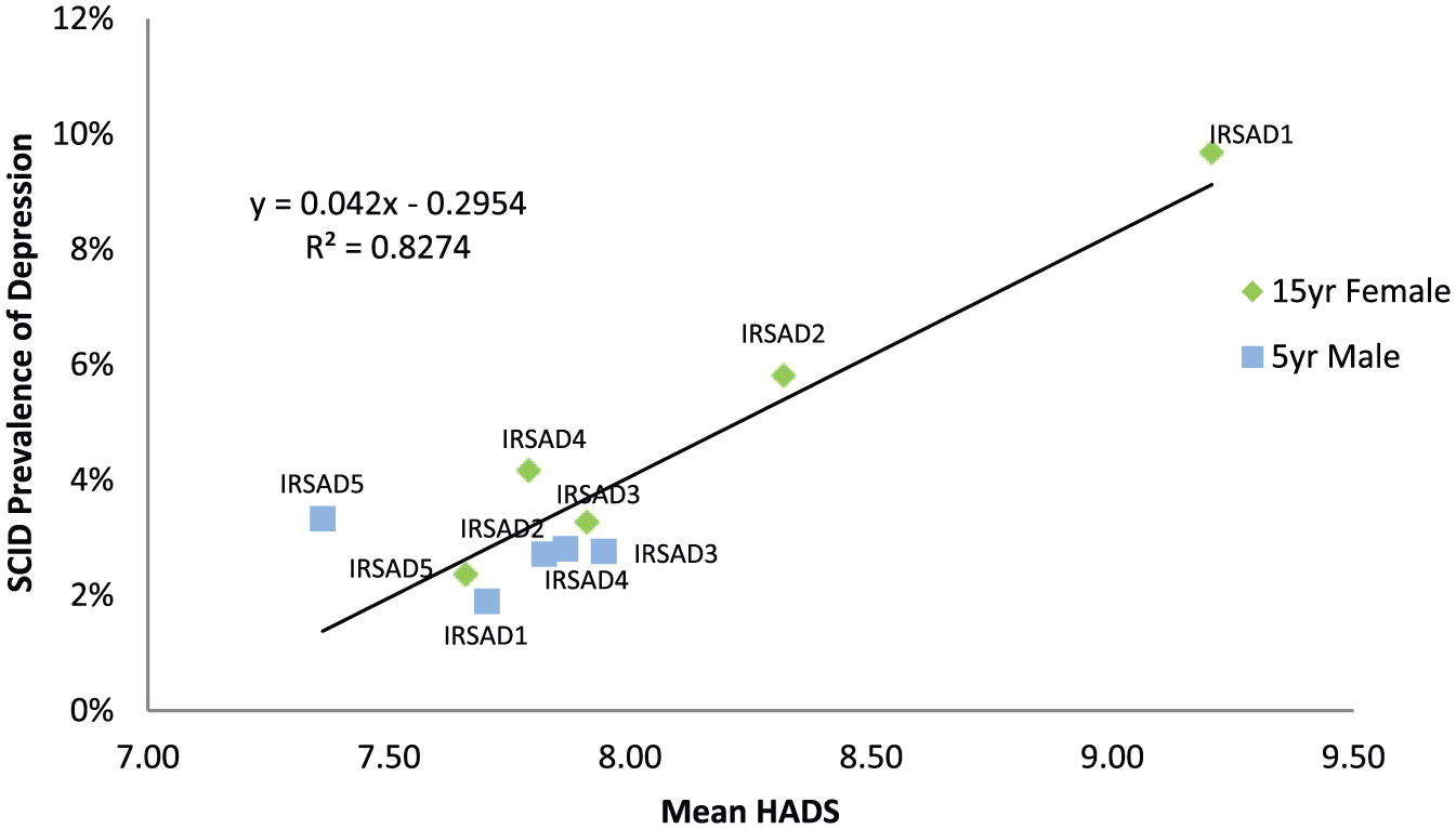
Regression between SCID depression prevalence and mean socio-economic status questionnaire scores from the 15-year female follow-up and 5-year male follow-up.
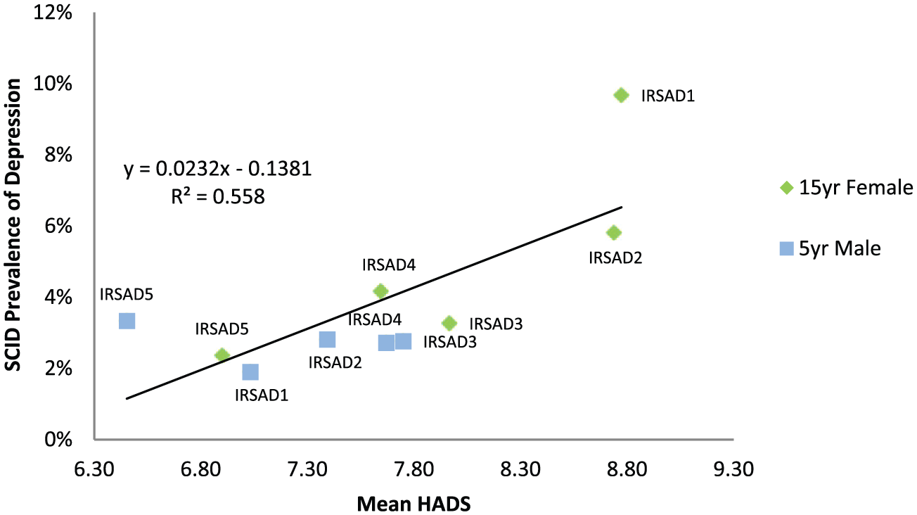
Regression between mean socio-economic status questionnaire score and SCID depression after removal of questionnaire scores of depressed individuals from the 15-year female follow-up and 5-year male follow-up.
GHQ-12 analysis by SES
There was a positive correlation between mean SES GHQ-12 scores and clinical depression (see Figure 6), when both the 10-year and 15-year female follow-up data were analysed separately (R2 = 0.61 and 0.76, respectively) and pooled (R2 = 0.73). The relationship was sustained following exclusion of questionnaire scores of those identified as meeting criteria for clinical depression (R2 = 0.49; see Figure 7). The predictions of the beta, gamma and Weibull models were moderate to good (R2 range of 0.39–0.75). The modelled prevalence variant of the beta distribution was superior to other models (see Table 3).
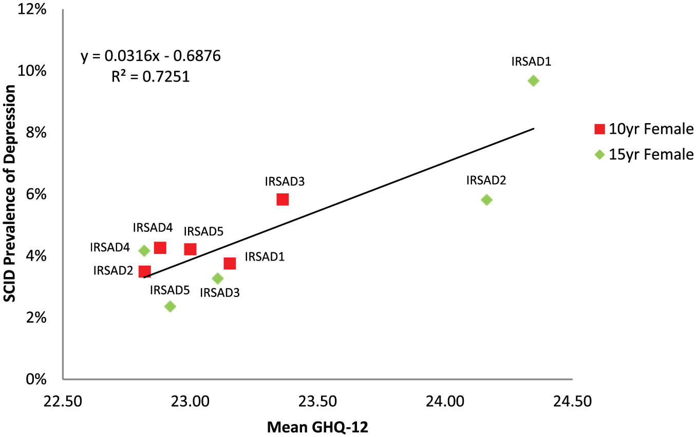
Regression between SCID depression prevalence and mean socio-economic status questionnaire scores from the 15-year female follow-up and 10-year female follow-up.
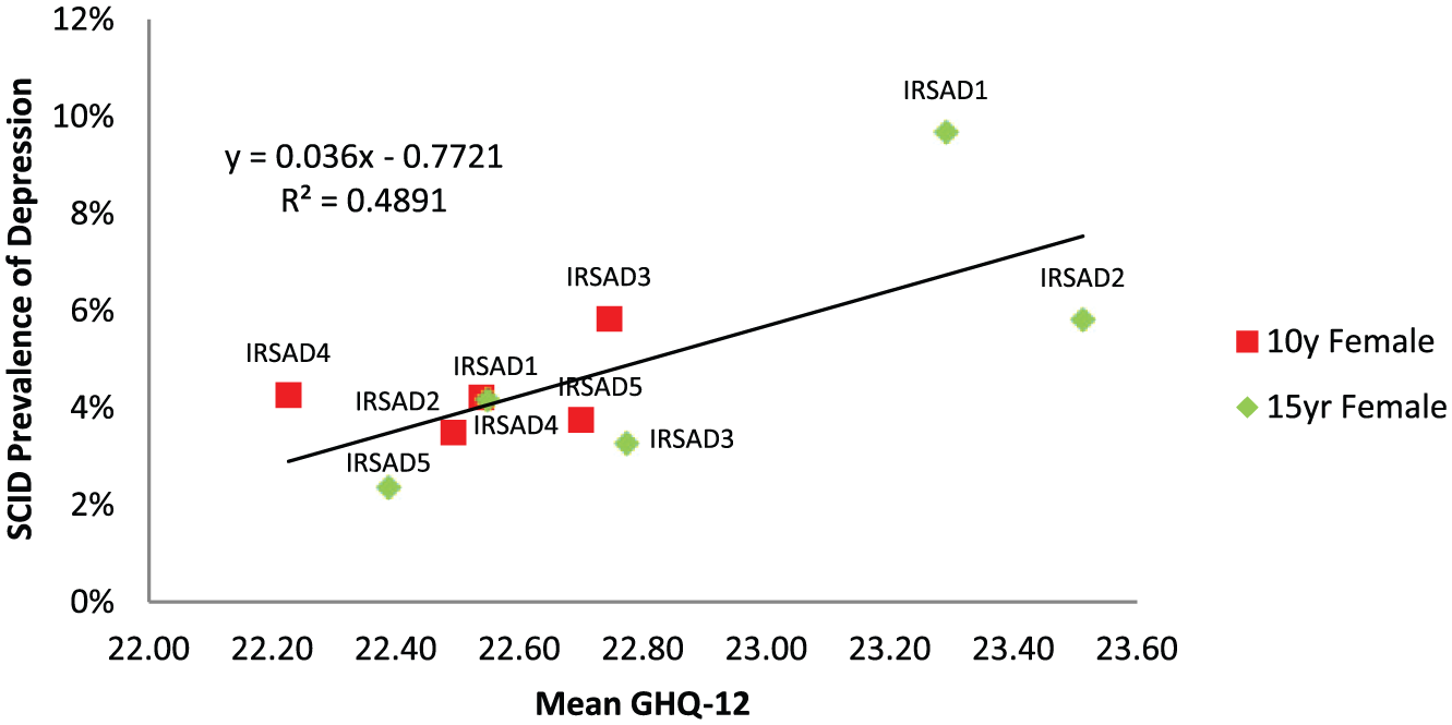
Regression between mean socio-economic status questionnaire score and SCID depression after removal of questionnaire scores of depressed individuals from the 15-year female follow-up and 10-year female follow-up.
Discussion
Here we examine, in an Australian context, whether the mean population mood can predict the prevalence of clinical depression. Overall, this study was able to demonstrate a relationship between mean population mood and clinical depression across socio-economic groups in women but not across age groups. This observation was robust across both the HADS and GHQ-12 questionnaires. We were unable to demonstrate the same association for the same using male data, although given our access to only a single cohort of male data (as opposed to two cohorts of female data), the lack of association should be interpreted with caution.
The strength of the relationships observed (R2: GHQ-12 0.73, HADS 0.83) compares favourably to the findings of other authors: Veerman et al. (2009) reported a R2 of 0.84 when regressing BDI scores and interview-diagnosed depression (Veerman et al., 2009); Rose and Day (1990) found R2 values of 0.78–0.97 between blood pressure, BMI, alcohol intake and sodium intake and their respective unhealthy degrees of excess (hypertension, obesity, high alcohol intake and high sodium intake; Rose and Day, 1990). In a UK-based study involving over 18,000 children, Goodman and Goodman (2011) found a R2 of 0.89–0.95 between Strengths and Difficulties Questionnaire (SDQ) scores and Development and Well-being Assessment (DAWBA) diagnosed child mental health disorders, decreasing to 0.76–0.88 after exclusion of children with mental health disorders; this study included other mental health illnesses and not just depression. However, one cross-national study based in seven countries found a poor correlation between SDQ and DAWBA scores (0.29–0.56) and cautioned cross-national questionnaire mean differences poorly translate into differences in mental illness prevalence (Goodman et al., 2012). Other studies report the existence of subsyndromal disease (e.g. Ayuso-Mateos et al., 2010) but do not report an explicit R2 regression value with which we can compare our study to.
Strengths and limitations
The gold standard for the diagnosis of depression is considered to be via structured clinical interview. However, as this is time-consuming, screening is generally performed with a questionnaire. One of the advantages of using GOS data is that mental health has been measured using both methods. This has allowed us to identify subclinical variants of low mood and not merely clinical cases of depression and dysthymic disorder. The GOS used a robust sampling methodology that utilised the electoral roll as the sampling frame, generating a study population whose baseline characteristics were similar to the general Australian population (Pasco et al., 2012).
There are also limitations to consider when interpreting our data. Outliers were evident in both the youngest and oldest age groups, with a clear trend absent across the age groups. Smaller sample sizes in these age groups are a likely contributing factor. For example, using 5-year cut-offs instead of 20-year cut-offs may have ameliorated this disparity and improved sensitivity by increasing the number of data points per analysis. However, increasing the number of age groups could increase the influence of random effects due to the smaller number of participants per group. We also note the natural history of a longitudinal study is fewer participants in older age groups due to mortality over time. As such, this may reflect real differences in the population rather than statistical anomalies.
A significant limitation to our study was that both questionnaire scores have a primary focus of evaluating psychological distress and have not been validated in measuring positive emotional states. For example, the GHQ-12 has been argued to contain three factors by Graetz (1991): anxiety, social dysfunction and lack of confidence. The HADS is a two-factor scale measuring anxiety and depressive qualities (Bjelland et al., 2002). The use of these scales is analogous to using a sphygmomanometer whose lowest blood pressure measurement is arbitrarily capped at 120 mmHg: these scales do not capture the ‘positive’ half of the mood distribution. This arguably strengthens the validity of our finding, as a more robust scale may demonstrate a stronger relationship between mean population mood and depression prevalence. For example, the Warwick–Edinburgh Mental Well-being Scale explicitly aims to measure positive aspects of mental health and has been extensively validated in UK populations (Tennant et al., 2007).
Furthermore, the screening questionnaires used may not have been equally appropriate for all age groups. The HADS has been reported not to perform as well in the elderly (Roberts et al., 2014; Samaras et al., 2013), although this has been contested by others (Boyes et al., 2013; Helvik et al., 2011). There is similarly ambivalence surrounding the GHQ-12, with at least one Australian study claiming it performs poorly in the elderly (Donath, 2001). The proportion of women meeting the criteria for depression, in particular dysthymia, in the <40-year age group was high. This may represent differences in perception of depressive symptoms or reporting stigma in this age group.
Given the GOS is an ongoing, population-based study, we cannot exclude the possibility of differential loss to follow-up impacting on the findings. For women, we utilised data from two time points (10-year and 15-year), which involved the same individuals: we assumed for simplicity that they constituted independent populations, but the validity of this assumption is unclear. However, population homogeneity would lead to an underestimation of interpopulation differences and so should reinforce the correlations we found rather than detract from them. Additionally, taxometric analysis within essentially the same population may also have led to groups who were so culturally and geographically similar that they failed to show population differences.
It should be noted that we used depression screening questionnaires as a surrogate measure for population mood, but it would be more accurate to describe them as measuring psychological distress. To contrast, the BDI used by Veerman et al. (2009) focuses on the negative symptomatology of depression alone (Beck and Beck, 1972). We speculate that, as it focuses specifically on depression, the BDI may have been superior for this study. The inclusion of non-depression-related items in the HADS and GHQ-12 may have masked the relationship between mean subpopulation group and depression prevalence by inflating questionnaire scores in populations with low depression prevalence. Despite this, individuals with depression have been shown to report higher levels of psychological distress, and psychological distress is a property of all individuals of a population, so Rose’s theorem should still hold true despite this distinction (Department of Health and Ageing, 2008).
Implications
The implication of our findings is that the prevalence of depression depends on the living circumstances of the population from which the cases arise. Just as the proportion of persons with obesity seen to be related to the ‘obesogenic’ environment, so the number of persons with clinical depression may depend on a ‘depressogenic’ environment. Further research is required to identify the determinants and environmental exposures that influence the population mean mood and how they might be amenable to change. Our study was able to demonstrate an association between mean population mood and depression in women. We were not able to demonstrate the same relationship in men, possibly due to our access to the data of only a single male cohort. Further work is required to definitively confirm or refute this finding. Currently, the Australian Mental Health Strategy 2013 cites prevention and early intervention as one of its five priority areas (Department of Health and Ageing, 2013b). Despite this, the vast majority of implemented policies have expanded the coverage of mental health services to the clinically ill rather than preventing new cases. Our study suggests that efforts to shift the mean population mood may complement the preventive aspect that these measures neglect.
There is already strong evidence suggesting effective preventive interventions are possible. Recent Cochrane reviews found educating adolescents and postpartum women on the use of cognitive behavioural therapy (CBT), psycho-educational therapy and interpersonal or family therapy reduced the risk of depression for at least a year post-intervention (Merry et al., 2011; Trivedi, 2014). A recent meta-analysis of randomised control trials found that depressive symptoms in the workplace could be reduced by the teaching CBT techniques to all workforce members (Tan et al., 2014). There is a plethora of work establishing individual risk factors for depression, such as parenting styles, adverse life events, societal wealth inequality, diet, smoking and exercise, which could also serve as targets for policy (Jacka et al., 2013; Pasco et al., 2008, 2011; Yap et al., 2014). It should be stressed that many of these are already targeted on the individual level (e.g. social workers assisting the financially disenfranchised). Our study encourages the theory that tackling these issues on a population scale would be beneficial; the ACE Prevention study found that certain population-level interventions (i.e. taxes/subsidies and regulation) would not only be effective but also cost-saving to the Australian health-care sector (Vos et al., 2010).
The authors note care must be taken when designing a potential intervention not to exacerbate pre-existing inequalities. As per Rose’s Paradox of Prevention, the majority of cases arise from large numbers of low-risk individuals compared to a small number of high-risk individuals (Rose and Day, 1990). Low-risk individuals are also the least likely to engage voluntarily in interventions as the benefit to each individual is small. Moreover, in the context of depressive disorders, there are further barriers to help-seeking. Individuals with mental illness tend to be of lower SES, low levels of education and have poorer housing situations (World Health Organization in Collaboration with the University of Melbourne, 2004). People with mental health disorders also face significant stigma, and less than half of people with a single mental health disorder were utilising health services in the most recent National Survey of Mental Health and Wellbeing in 2007 (Department of Health and Ageing, 2008; Reavley and Jorm, 2012). As such, the authors note that the most successful interventions would be blanket interventions that do not entail financial input or proactive volunteering from participants (e.g. school-based programmes which teach psychoeducation or CBT training). Interventions that reduce exposure to environmental determinants would also reduce rather than exacerbate inequality.
Additionally, if a relationship exists between the mean mood and depression, it is possible that similar phenomena exist for other mental health conditions. One study based in Norway has established a link between population mean frequency of gambling and the proportion of not only heavy gamblers but also moderate gamblers compared to infrequent gamblers (Hansen and Rossow, 2012). As previously described, the prevalence of heavy drinking is known to correlate with the population mean alcohol intake (Rose and Day, 1990). It seems reasonable to speculate that alcohol abuse or dependence exhibit similar correlations. Another logical connection would be between anxiety and psychological distress: there is limited evidence that this may be the case. Anxiety disorders are the most prevalent type of mental illness in Australia (Reavley et al., 2011). The National Survey of Mental Health and Wellbeing reported the clinically anxious are twice as likely to have very high levels of psychological distress compared to the general population (Department of Health and Ageing, 2008). A recent Cochrane review also found that treatment of anxiety reduces psychological distress (Donker et al., 2009). Future research could investigate this link. Correlations between other mental illnesses such as schizophrenia and bipolar affective disorder may also exist, but it is less clear what population attribute of ‘normality’ would be associated with these.
Conclusion
Here, we show that the mean population mood is strongly correlated with the population prevalence of depression in Australia in women. We were unable to demonstrate the same relationship in men, but given our limited data for men in this study, this should be interpreted with caution. Further work to identify population determinants of mean mood could create policy targets to reduce the prevalence of depression. We note that further research could explore the relationship between psychological distress and other mental health illnesses, such as anxiety disorders.
Footnotes
Acknowledgements
J.L.V. devised the project design and provided feedback on drafts; L.J.W., J.A.P., F.N.J. and S.L.B. provided the data; and A.D.S. was responsible for data analysis and writing the paper. All authors provided intellectual input and approved the manuscript for submission.
Declaration of Conflicting Interests
The author(s) declared no potential conflicts of interest with respect to the research, authorship and/or publication of this article.
Funding
The authors received no financial support for the research, authorship and/or publication of this article: The Geelong Osteoporosis Study is supported by the NHMRC (project #628582). LJW is supported by a NHMRC Career Development Fellowship (1064272). FNJ has received Grant/Research support from the Brain and Behaviour Research Institute, the National Health and Medical Research Council (NHMRC), Australian Rotary Health, the Geelong Medical Research Foundation, the Ian Potter Foundation, Eli Lilly, the Meat and Livestock Board, Woolworths Limited, Fernwood Gyms and The University of Melbourne and has received speakers honoraria from Sanofi-Synthelabo, Janssen Cilag, Servier, Pfizer, Health Ed, Network Nutrition, Angelini Farmaceutica, Eli Lilly and Metagenics. She is supported by an NHMRC Career Development Fellowship (2) (#1108125).
References
Supplementary Material
Please find the following supplemental material available below.
For Open Access articles published under a Creative Commons License, all supplemental material carries the same license as the article it is associated with.
For non-Open Access articles published, all supplemental material carries a non-exclusive license, and permission requests for re-use of supplemental material or any part of supplemental material shall be sent directly to the copyright owner as specified in the copyright notice associated with the article.