
Abstract
Two-dimensional correlation spectroscopy (2D-COS) is a technique that permits the examination of synchronous and asynchronous changes present in hyperspectral data. It produces two-dimensional correlation coefficient maps that represent the mutually correlated changes occurring at all Raman wavenumbers during an implemented perturbation. To focus our analysis on clusters of wavenumbers that tend to change together, we apply a k-means clustering to the wavenumber profiles in the perturbation domain decomposition of the two-dimensional correlation coefficient map. These profiles (or trends) reflect peak intensity changes as a function of the perturbation. We then plot the co-occurrences of cluster members two-dimensionally in a manner analogous to a two-dimensional correlation coefficient map. Because wavenumber profiles are clustered based on their similarity, two-dimensional cluster member spectra reveal which Raman peaks change in a similar manner, rather than how much they are correlated. Furthermore, clustering produces a discrete partitioning of the wavenumbers, thus a two-dimensional cluster member spectrum exhibits a discrete presentation of related Raman peaks as opposed to the more continuous representations in a two-dimensional correlation coefficient map. We demonstrate first the basic principles of the technique with the aid of synthetic data. We then apply it to Raman spectra obtained from a polystyrene perchlorate model system followed by Raman spectra from mammalian cells fixed with different percentages of methanol. Both data sets were designed to produce differential changes in sample components. In both cases, all the peaks pertaining to a given component should then change in a similar manner. We observed that component-based profile clustering did occur for polystyrene and perchlorate in the model system and lipids, nucleic acids, and proteins in the mammalian cell example. This confirmed that the method can translate to “real world” samples. We contrast these results with two-dimensional correlation spectroscopy results. To supplement interpretation, we present the cluster-segmented mean spectrum of the hyperspectral data. Overall, this technique is expected to be a valuable adjunct to two-dimensional correlation spectroscopy to further facilitate hyperspectral data interpretation and analysis.
This is a visual representation of the abstract.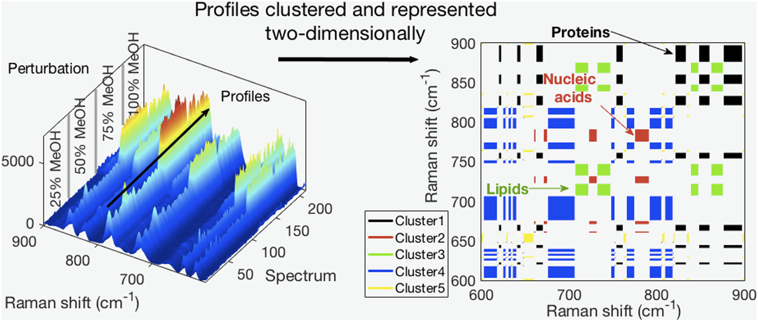
Keywords
Introduction
Changes that occur in a sample over time or in response to some experimental treatment, a perturbation, are common targets of spectral analysis. These changes are often probed using Raman spectroscopy, an information-rich optical technique especially suitable for use with biological samples.1–7 These include that the macromolecular compositional changes occurring in human embryonic stem cells undergoing differentiation exhibit an increase in protein content relative to that of nucleic acids, 8 in Chinese hamster ovary cells, lipid content increases in late stages of apoptosis, 9 in red blood cell concentrates stored in transfusion bags, oxyhemoglobin and lactate levels increase with storage time while glucose levels decrease,10–12 and the hydrolysis of peptide bonds is observed at high temperature in freeze-dried tissue. 13
A well-established technique to examine the synchronous (in-phase) and asynchronous (out-of-phase) changes observed between different peaks in Raman spectra that occur in the course of a perturbation is two-dimensional correlation spectroscopy (2D-COS). 14 2D-COS is based on the analysis and two-dimensional representation of covariances and correlation coefficients that reveal correlated synchronous changes between peaks while the application of the Hilbert–Noda transform permits an examination of asynchronous changes.14,15 2D-COS is used to understand the relationship between peaks, 12 to identify the types of macromolecule that contribute to peaks,16,17 to assess the correspondence between Raman peak changes and bioanalytical measurements,12,18 to gain insight into structural changes in molecules, 19 and to analyze kinetic processes. 20 However, synchronous or asynchronous changes, even though highly correlated, may not show the same qualitative profile or trend across the perturbation.
Due to their highly complex composition, the interpretation of Raman spectra from cells can be particularly challenging, a situation mitigated by the fact that many peaks repeatedly represent each of the few major macromolecules (lipids, proteins, nucleic acids, and carbohydrates21,22) that make up more than 85% of the dry weight of cells. 23 The peaks pertaining to each type of macromolecule can, in general, be expected to vary together. In particular, peaks that vary together should exhibit highly similar profiles and clustering techniques can be used to group them. Though complex changes should generally be expected, focusing on the limited number of major macromolecules provides a starting point from which subtler changes can be unraveled and, in conjunction with 2D-COS, the interpretation of Raman spectra can be improved.
K-means clustering is a method to partition an n-dimensional population into k clusters such that for every cluster the distances between cluster members are less than the distances between clusters.24–26 For example, it can be done based on Raman spectra to segment images, 27 classify molecular structures, 28 used in conjunction with principal component analysis (PCA) to extract cluster spectral information, 29 and separate healthy from breast cancer tissues. 30 Though normally applied to the spectra themselves, we report here on a method to use k-means clustering on the profiles at all the wavenumbers in a hyperspectral data set to group similar profiles. The cluster memberships are then displayed two-dimensionally in a manner analogous to a two-dimensional correlation coefficient map to create a two-dimensional cluster member spectrum (2D-CMS). A 2D-CMS shows which Raman peaks change similarly based on the clustering of their profiles rather than a similarity based on the correlation coefficients between their profiles.
We use synthetic “spectra”, each with eight peaks and simple profiles as described further below, to explain the principles and application of the method. We then apply the method to experimentally obtained Raman spectra. First, we use a relatively uncomplicated model system of polystyrene beads submerged in a NaClO4 solution to assess and demonstrate its utility for the analysis of spectroscopic data. 31 By scanning from the center across the edge of a polystyrene bead cluster, the polystyrene peak intensities would decrease while those of the perchlorate ion would increase, thus producing contrary profiles. We then extend the application to the more challenging case of spectra obtained from mammalian cells fixed with different percentages of methanol. Because methanol is a fixative used for cells that coagulates proteins and also dissolves lipids from cell membranes, 32 varying the percentage of methanol used for cell fixation would induce different profiles in the macromolecules of cells.
Methods
Two-Dimensional Correlation Spectroscopy.14,15 Two-dimensional correlation spectroscopy (2D-COS) is a well-known analysis technique with various implementations17,18,33–36 and several reviews and tutorials are available about its principles and applications.14,15,19,37–42
Perturbation Domain Decomposition.43,44 Perturbation domain decomposition (PDD) unfolds profiles during calculation from 2D-COS maps, that is, from two-dimensional correlation spectra (2D-COV) and two-dimensional correlation coefficient maps (2D-COR) by augmenting the spectra, before calculating the maps, with a sequence of single channel delta functions at successive channels—one for every perturbation stage. This produces profiles similar to those of the measured data, but they are directly commensurate with the 2D-COS maps, for example, being mean centered and scaled. The profiles so extracted can then be used separately or as part of an extended 2D-COS map to aid the interpretation of 2D-COS features.
K-Means Clustering.24–26 K-means clustering is an unsupervised partitioning procedure. To perform k-means clustering, the number of clusters, k, must be specified at the outset. Every profile in a data set is then assigned to exactly one of a number of non-empty clusters by an iterative procedure. Initial cluster “cores” or centroids start with k profiles randomly selected from the data set and the distance between every profile and every centroid is determined using one of a number of distance measures. Every profile is then assigned to the cluster of its nearest centroid and thereafter every centroid is modified such that it is now the mean profile of all the members of its cluster. Because the centroids have changed from their initial values, the distances between every profile and every centroid might now be different and they are recalculated. For the same reasons, some profiles might now be reassigned to different clusters and the resultant changes in cluster members produce further centroid modifications as they now are the new means of the cluster members. This procedure is repeated until profiles no longer change clusters or a specified iteration number is reached. A difficulty that may arise using this procedure is that, depending on the initial selection of centroids, clustering might converge to a local minimum. It might also be unclear on what basis to specify the best number of clusters to use for a given task though an inspection of the distribution of cluster members might show whether effective clustering was obtained and, by extension, whether the number of clusters chosen was appropriate.
Two-Dimensional Cluster Member Spectra. Separately, for each of the data sets, a 2D-COR with PDD is performed and the profiles at all the channels or wavenumbers are partitioned with k-means clustering into groups of similar profiles. This can also be done without performing a 2D-COR associated PDD by using the standard normal variates of the profiles. Importantly, constant peak profiles are mean centered and thus would be zero and coincide with zero baseline profiles. Peaks are identified by a mean profile that exceeds a small threshold, for instance, based on the limit of detection (LOD) criterion. 45 Before clustering, peaks that are constant (e.g., fluctuating with a standard deviation < LOD/3) are added back into the PDD at a constant level that exceeds the LOD, for example, 10% of the maximum absolute PDD value. Baseline profiles (mean profiles < LOD) are set to zero. Constant profiles cannot feature in analyses based on correlation coefficients because their standard deviations are zero and the calculation of correlation coefficients involve division by the standard deviation.
Cluster-Segmented Spectra. Besides the generation of a 2D-CMS from the clustering of profiles in Raman hyperspectra, cluster-segmented spectra can be generated for all the spectra. A cluster-segmented spectrum shows which channels or wavenumbers of a spectrum belong to the same cluster. This is done, for example, by differential color coding of all the wavenumbers of the data set mean spectrum that belong to the same cluster.
Synthetic Spectra. Nine spectra of 1610 channels were simulated each consisting of eight rectangular “peaks” with a width of 100 channels. They were centered at channels 100, 300, 500, 700, 900, 1100, 1300, and 1500 and labeled in the same order from Peak 1 (P1) to Peak 8 (P8). The maximum intensity of the first five peaks was 1 and that of the remaining three peaks was 0.5. P1 decayed exponentially by 50% of its initial value at each perturbation stage; P2 increased linearly from 0 to 1.00; P3 was present only at stages 4 (intensity 0.8), 5 (intensity 1.0), and 6 (intensity 0.8); P4 increased linearly from 0 at stage 1 to 1.0 at stage 8 and then remained at 1 for stage 9. P5 was constant at 1.0 throughout all perturbation stages. P6 decreased by 50% at each stage starting at an intensity of 0.5. P7 decreased linearly from 0.5 to 0 and P8 was also constant, but at intensity 0.5. These peaks are shown in Fig. 1a and their profiles in Fig. 1b. The profiles of these peaks constitute six distinct clusters. (a) Surface plot of eight synthetic peaks (P1 to P8) that change in a correlated, anticorrelated, or independent manner. (b) Profiles of individual peaks.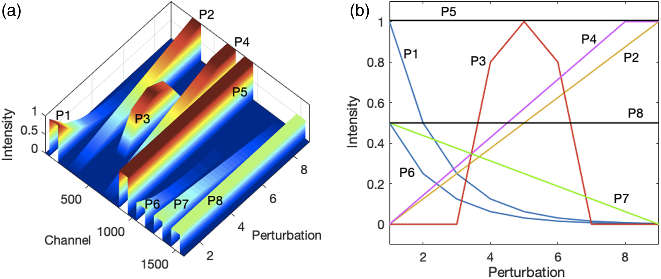
Polystyrene Perchlorate Model System.
31
The method was applied to a model system consisting of an aqueous suspension of ∼10 μm diameter polystyrene carboxylated microspheres (Sigma-Aldrich, US) that was deposited on a 12.5 mm diameter glass-encapsulated gold mirror (ThorLabs, US) with the mirror placed in a Petri dish and then submerged in 2.5 M NaClO4. To obtain spectra, we scanned across the edge of a close-packed area of beads where a transition from a beaded to a bead-free area occurred as shown in Fig. 2a. The scanning produced increasing perchlorate ion and decreasing polystyrene peak intensities, thus producing opposite profiles. The perchlorate ion is insoluble in the polystyrene beads and its major Raman band at ∼935 cm−1 is well separated from strong polystyrene Raman bands as evident in Fig. 2b. The Petri dish containing the mirror with beads was placed under a confocal Raman microscope (InVia, Renishaw, Gloucestershire, UK) and a water-immersion 40× (0.80 NA, 3300 µm working distance; Leica Microsystems, Germany) objective lens used to focus the laser beam to a spot of approximately 3 µm × 30 µm. Thirty-eight Raman spectra, one per step, with 1s per spectrum were collected at room temperature while moving in ∼1 µm steps through the edge of the bead array. A 50 µm slit width, 785 nm excitation, and ∼80 mW power at the sample were used. (a) Image of polystyrene perchlorate model system showing the line scan performed from left to right. (b) Raman spectra from the model system, spectra were not normalized. (c) Constant sum normalized Raman spectra from Jurkat cells fixed with different percentages of methanol.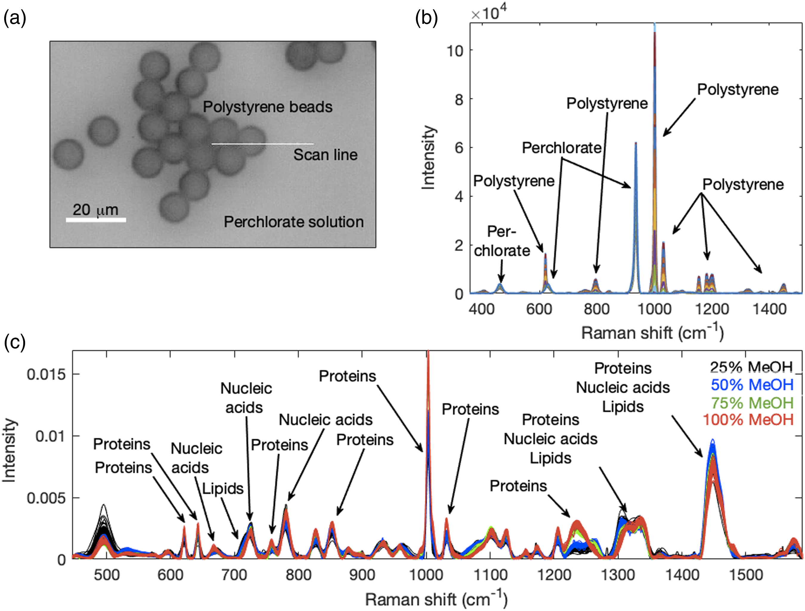
Cell Culture and Fixation. T-75 flasks containing 15 mL Immunocult-XF medium (Stemcell Technologies, Canada) supplemented with 1X antibiotic–antimycotic cocktail (Gibco, US) were seeded with 2*106 Human Jurkat T-cells (ATCC, TIB-152). Thereafter, they were incubated in a humidified incubator at 37 °C and 5% CO2 for 72 h. When exponentially growing, cells were harvested and fixed for Raman spectroscopy.
Four groups of approximately 2 × 10⁶ cells were collected and centrifuged for fixation with different volumes (12.5, 25, 37.5, or 50 μL) of methanol where smaller volumes of methanol were augmented with water to 50 μL, to perform fixation in 25, 50, 75, or 100% methanol. The supernatant was removed, and the cells were washed once with saline. The washed cell pellets were then resuspended in one of the given amounts of methanol and incubated at −20 °C for 20 min. The cell/methanol suspension was then pipetted onto 12.5 mm diameter glass-encapsulated gold mirrors (ThorLabs, US) and allowed to air-dry in a biosafety cabinet with no further manipulation. The fixed cell samples were then stored at 4 °C until Raman spectra were collected.
Mammalian Spectra. Approximately 55 Raman spectra were measured from each of the four groups of fixed samples. The spectra were acquired in map acquisition mode using a 50× objective lens (Leica Microsystems, Germany) with 10 s acquisition time per spectrum with each spectrum containing information from 10 to 15 cells. These spectra with some macromolecular peak identities are shown in Fig. 2c. Various literature sources are available where Raman band assignments can be found.7,46
Data Generation and Processing. Matlab R2017b (The MathWorks Inc., US) was used to generate synthetic data, for spectral processing, and for data analyses. Raman spectra were preprocessed with an automated moving average-based baseline-flattening method (15 iterations), 47 a two-dimensional second difference cosmic ray-induced spike removal method 48 and a contiguous single-channel Voigt distribution fitting method for smoothing. 49 2D-COS computations were implemented with Matlab and the Matlab kmeans function with Euclidean distance measure was used for k-means clustering.
Results and Discussion
Demonstration of 2D-CMS. To orient the reader, we briefly discuss some aspects of the 2D-COS for the synthetic data. The 2D-COV is shown in Fig. 3a and the 2D-COR in Fig. 3b. P1 and P6 have identical exponentially declining profiles even though the P6 intensities are only 50% of the P1 intensities. Thus, modest positive 2D-COV cross-peaks are observed at channels 100 × 1100 and 1100 × 100 but perfect correlation coefficients in the 2D-COR. P1 and P2 change in opposite directions because the P2 profile increases linearly. Thus, the 2D-COV and 2D-COR channel 100 × 300 and 300 × 100 cross-peaks are negative. The P3 profile is symmetric around perturbation stage 5; thus, the increasing first half of the profile changes inversely to the sharp exponential drop of the corresponding part of P1, while its decreasing second half changes in concert with the corresponding part of the P1 profile, but with the latter now exponentially declining with very low intensities and the net result being negative 2D-COV and 2D-COR channel 100 × 500 and 500 × 100 cross-peaks. Proceeding likewise, all the cross-peaks can be interpreted in the standard 2D-COS manner, keeping in mind that the P5 and P8 profiles are constant thus the rows and columns at channels 900 and 1500 will have no cross-peaks due to zero covariations (2D-COV) and undefined correlation coefficients (2D-COR) with themselves and other profiles. 2D-COS and 2D-CMS performed on synthetic data. (a) The 2D-COV and (b) 2D-COR for the synthetic data. (c) Using k-means clustering, the profiles of the eight synthetic peaks (P1 to P8), shown in Fig. 1b, were grouped into six clusters. (d) The 2D-CMS shows the cluster auto- and cross-peaks between cluster members. The 2D-CMS displays in (d) as green squares cluster membership between the constant profiles of Cluster 3, whereas the green circles in (b) show where the 2D-COR does not display a correlation coefficient because these are constant profiles. The 2D-COR also displays a relatively high correlation coefficient between the profiles of Clusters 2 and 6 as shown by the reddish squares highlighted by magenta circles in (b), but in the 2D-CMS they are assigned to different clusters as shown by the red and magenta squares, respectively, in (d) thus no cluster cross-peaks occur between them as shown by the empty magenta circles.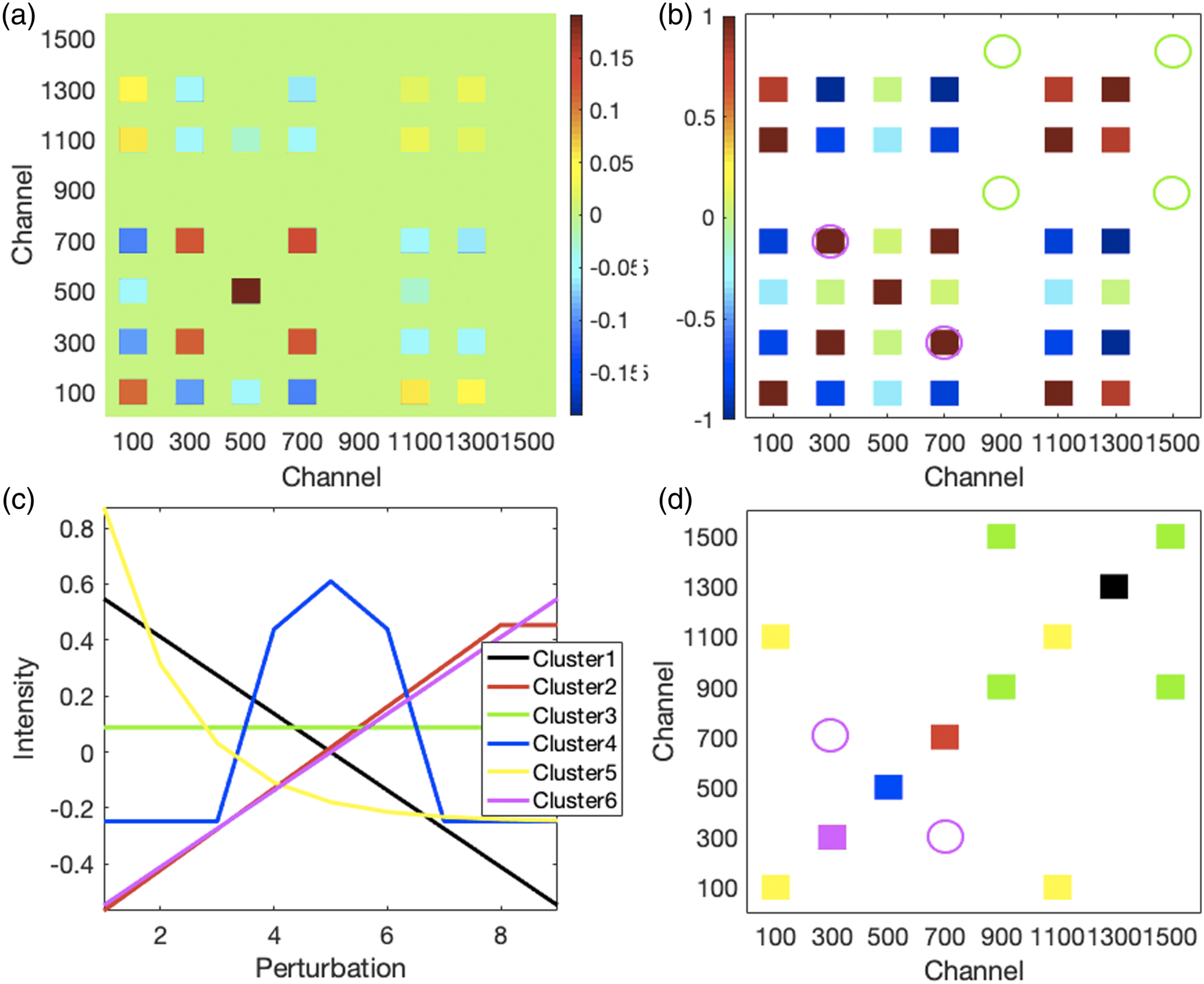
Performing six-cluster k-means clustering on the decomposed perturbation domain profiles of the synthetic data produced six centroids with profiles that correctly matched those of the peaks in each cluster shown in Fig. 3c. The 2D-CMS is shown in Fig. 3d. Consistent cluster colors are used for Figs. 3c and 3d (ordering of clusters occur randomly). In Fig. 1a, P1 has the same profile as P6 (assigned to Cluster 5 in Fig. 3c). Both decline exponentially, but from different initial intensities. Thus, the 2D-CMS in Fig. 3d shows yellow squares at channels 100 × 100 and 1100 × 1100 where P1 and P6, respectively, cluster with themselves. Yellow squares also occur at channels 100 × 1100 and 1100 × 100 showing that P1 and P6 cluster together. Since P2 is the only member of Cluster 6, it is represented by only one 2D-CMS square (magenta) at channels 300 × 300 where it clusters by itself. This is also true for P3 (blue), P4 (red), and P7 (black) at 500 × 500, 700 × 700, and 1300 × 1300, respectively. P5 and P8 do not change, thus have constant profiles that were assigned to Cluster 3 (green). As for P1 and P6 above, in Fig. 3d the 2D-CMS shows with green squares at channels 900 × 1500 and 1500 × 900 that P5 and P8 have the same cluster membership.
The sparsity of the 2D-CMS that is focused on identifying clusters of synchronously changing peaks contrasts sharply with the synchronous 2D-COS maps. The 2D-COV in Fig. 3a and the 2D-COR in Fig. 3b include numerous auto- and cross-peaks with various degrees of mutual covariance and correlation between peaks. An important advantage of the 2D-CMS is that constant profiles, as shown by the Cluster 3 profile in Fig. 3c, are clustered and represented in a 2D-CMS, for example, green squares in Fig. 3d. They are not present in the corresponding 2D-COR as shown by the green circles because a constant profile does not have a defined standard deviation and the correlation coefficients between constant profiles cannot be determined. Indeed, the correlation coefficient between any profile and a constant profile cannot be determined as evidenced by the empty rows and columns along channels 900 and 1500 in Fig. 3b. Being able to include constant profiles in the segmentation or grouping of peaks, provided that baseline profiles are treated separately, aids in analysis by permitting unchanging peaks to be distinguished from others. However, including constant profiles actually reduces the 2D-CMS matrix sparsity.
Another difference underlying the sparsity effect is that profiles may be relatively highly correlated yet belong to different clusters when the differing characteristic features of their profiles can be more readily captured by a clustering procedure (that correlation coefficients are not designed to do). Thus, Clusters 3 and 5 (green and yellow, respectively) each have two autopeaks (i.e., there are two green peaks and two yellow ones on the diagonal) signifying two members in each cluster. On the other hand, though strong correlation coefficients are observed for the profiles at channels 300 and 700 (highlighted by the magenta circles in Fig. 3b), they belong to different clusters, those being the Fig. 3c Clusters 6 (magenta) and 2 (red). Consequently, there are no corresponding “cross-clusters” (i.e., indicating joint cluster membership) for these profiles in Fig. 3d (magenta circles). Relatedly, unlike 2D-COS and principal components in PCA, clusters cannot contain anticorrelated elements and there are no negative clusters. These effects contribute to the general sparsity observed in 2D-CMS.
The asynchronous results of performing a six-cluster k-means clustering are shown in Fig. S1 (Supplemental Material). Besides spectral resolution enhancement, the asynchronous 2D-COS maps represent phase differences between profiles and are useful for inferring the sequential order of spectral events. 50 Applying the Hilbert–Noda transform 15 changes the correlations between profiles, thus the asynchronous 2D-COS maps differ from the synchronous 2D-COS maps. However, we think it unlikely that the transform would change cluster memberships, as shown in Fig. S1, where the “asynchronous” 2D-CMS is identical to the “synchronous” 2D-CMS.
Application of 2D-CMS. To illustrate the application of 2D-CMS to Raman spectra, we used a model system of polystyrene beads submerged in a sodium perchlorate solution. Scanning from the beads, where polystyrene is present and some perchlorate is covering the beads, to the bead-free area where only perchlorate is present (Fig. 2a) produced decreasing polystyrene Raman bands and increasing perchlorate Raman bands. In Fig. 4, we show 2D-COS and 2D-CMS maps of a spectral region of interest of the Fig. 2b Raman spectra that contains the major polystyrene and perchlorate bands. Because the polystyrene and perchlorate peaks in this model system changed in an opposite manner, all the negative peaks in the 2D-COS and 2D-COR maps (Figs. 4a and 4b, respectively) are cross-peaks between polystyrene and perchlorate Raman bands. Hence, the simplicity of this model system permits the use of positive and negative peaks to identify peaks belonging to each of the two components present. We focus on the 800 cm−1 to 1200 cm−1 region containing the major autopeaks of polystyrene (at ∼1002 cm−1) and perchlorate (at ∼935 cm−1). They are shown by arrows in Figs. 4a and 4b, and a cross-peak between them with blue (Fig. 4a) and cyan (Fig. 4b) arrows. 2D-COS and 2D-CMS performed on a polystyrene perchlorate model system. (a) The 2D-COV and (b) 2D-COR maps for the model data. The major autopeaks for polystyrene and perchlorate are shown with arrows and a cross-peak between polystyrene and perchlorate is indicated by a blue or cyan arrow. The y-axis labels in (a) also apply to (b). (c) Using k-means clustering the PDD profiles of the model system peaks (Fig. 2b) were grouped into three clusters. The cluster legend applies to both (c) and (d). (d) The 2D-CMS shows the cluster auto- and cross-peaks between cluster members. For example, all the green rectangles indicate auto and cross-peaks, but they pertain only to the perchlorate ion bands. Because the very small perchlorate 1129 cm−1 peak is above the used threshold but not visible in the (a) and (b) top side panels that contain spectra, the 1129 cm−1 green rectangle auto cluster appears not matched to a peak. Unlike 2D-COS, where cross-peaks between polystyrene and perchlorate bands occur, there are no cluster cross-peaks between them because they are members of different clusters.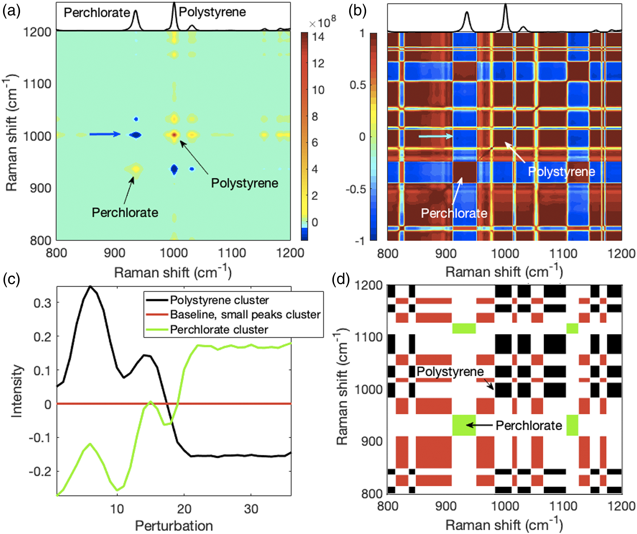
For the 2D-CMS processing, peaks below the LOD threshold were set to zero, thus very small peaks and baseline levels were constant. Clustering using three clusters produced the profile centroids in Fig. 4c. The sinusoidal changes in the centroid profiles for polystyrene and perchlorate are due to the spherical nature of the beads and how they were packed together. The 2D-CMS map in Fig. 4d distinctly shows peaks pertaining to perchlorate (green rectangles), polystyrene (black rectangles) and baseline levels with small peaks (red rectangles). In contrast to 2D-COS, there are no cross-clusters between any of the above three groups. Where cross-clusters do occur, they occur between Raman bands pertaining to the same group (e.g., only between polystyrene peaks). In 2D-COS, negative cross-peaks reveal that peaks change in an opposite manner, but in 2D-CMS such information must be determined from an inspection of the centroids.
We next performed 2D-COS and 2D-CMS on a more complex data set. This set contained spectra from fixed Jurkat cells. The results of an instructive subset of the entire measured spectral window, the 600 cm−1 to 900 cm−1 spectral region, is presented in Fig. 5 and the complementary section is shown in Fig. S2 (Supplemental Material). The 2D-COV and 2D-COR for this data set are presented in Figs. 5a and 5b, respectively. It is easier to identify related weak and strong peaks using the 2D-COR than the 2D-COV because the profiles are normalized to their standard deviations. However, this can make the 2D-COR map more complex. Thus, we discuss, only for orientation, the 2D-COV autopeaks and cross-peaks by proceeding along the y-axis 782 cm−1 row indicated by the left arrow. We use the peaks numbered along the mean spectrum (of the Fig. 2c cell spectra) shown in the top side panel of Fig. 5a. 2D-COS and 2D-CMS performed on Jurkat cell Raman spectra showing the 600–900 cm−1 spectral region; the complementary region is shown in Fig. S2 (Supplemental Material). (a) The 2D-COV and (b) 2D-COR for the spectra. The y-axis labels in (a) also apply to (b). Auto- and cross-peaks along the row indicated by the left arrow are discussed in the main text. (c) Shown are the PDD profile centroids for all wavenumbers from 600 cm−1 to 900 cm−1 that were k-means clustered into five groups intended to represent lipids, proteins, nucleic acids, carbohydrates, and other components. The cluster legend applies to both (c) and (d). The perturbation consisted of fixing cells with four different percentages of methanol. Approximately 55 spectra were obtained from each fixation. The x-axis shows the number of spectra in the set and the vertical lines indicate where the perturbation boundaries are. (d) Lipids, proteins, and nucleic acids were recognizably captured by the clustering process as revealed by the 2D-CMS cluster auto- and cross-peaks between cluster members. A comparison of (b) and (d) shows the complementary nature of 2D-COR and 2D-CMS. For example, the nucleic acid peaks that cluster together indicated by the dashed circles in (d) also have relatively high correlation coefficients as indicated by the same dashed circles in (b). In contrast, the 2D-COR can display relatively high correlation coefficients between nucleic acid and protein peaks as indicated by the square inside the upper dotted circle in (b) for the 782 cm−1 nucleic acid peak and the 854 cm−1 protein peak, but with 2D-CMS the protein peak is clustered with proteins and no cross-cluster exists as indicated by the upper dashed circle in (d). The solid circle in (b) shows that anti-correlations are evident in the 2D-COR, but they do not appear in the 2D-CMS as evident by the empty solid circle in (d). Anticorrelated profiles are assigned to different clusters and there are no “negative” clusters.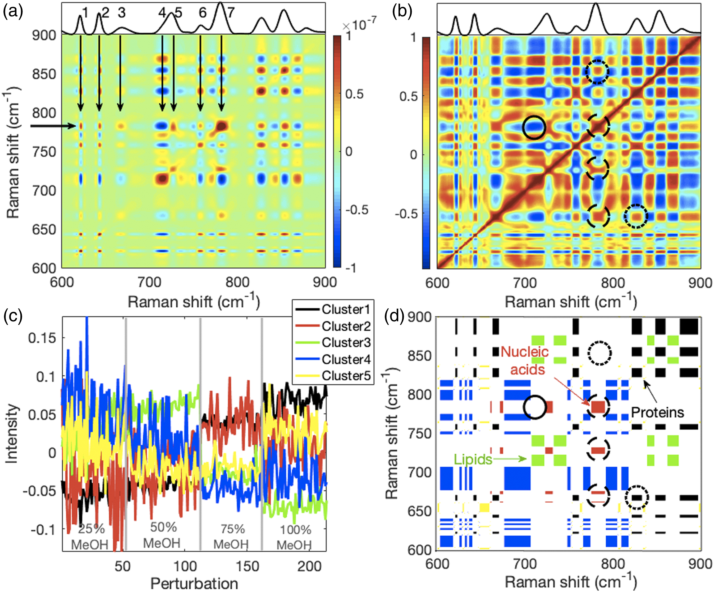
Peak 7 is a composite nucleic acid peak and its autopeak is prominent on the diagonal where the left arrow would intersect with the Peak 7 arrow. Peak 7 covaries positively (warm colors) with the protein Peaks 1 and 2 at 621 cm−1 and 643 cm−1, respectively, the 668 cm−1 nucleic acid Peak 3, the Peak 5 adenine part of the composite 720 cm−1 peak, and the tryptophan protein Peak 6 at 757 cm−1. Note that, without consulting band assignments, it is not possible to tell from 2D-COV which autopeaks and cross-peaks belong to the same macromolecules. Because methanol leaches lipids from cells but coagulates proteins 32 and compacts nucleic acid conformations, 51 cross-peaks related to lipids will covary inversely with those of proteins and nucleic acids. This is shown for the 714 cm−1 Peak 4 phosphatidylcholine part of the composite 720 cm−1 peak. Consequently, only contrary variations afford here some discrimination between macromolecules.
The 2D-CMS results for the cell spectra are presented in Figs. 5c and 5d. The PDD profiles consisted of four groups of spectra fixed with 25, 50, 75, or 100% methanol. They were k-means clustered into five clusters. The number of clusters was chosen to represent the major classes of macromolecules: lipids, proteins, nucleic acids, carbohydrates, plus one more for other components. The color-coded centroids of these clusters, across the four methanol percentages spanning all 214 spectra, are shown in Fig. 5c. The auto- and cross-clusters from the same clustering are shown in Fig. 5d with the same color coding. Three macromolecular groups, lipids, proteins, and nucleic acids, were most clearly separated (see Fig. 6c further below for the basis of the macromolecular group identification). These are shown as green, black, and red squares, respectively. Comparing the 2D-CMS with the 2D-COR, it can be seen, for example, that the same related nucleic acid peaks (782, 725, and 668 cm−1) represented by red squares inside the dashed circles of Fig. 5d are evident as reddish squares of high correlation coefficients inside the dashed circles of Fig. 5b. (a) The cluster-segmented mean spectrum of the Figs. 3c and 3d clustered and identically color-coded synthetic data shows which two peaks belong to one of two clusters (yellow, green) and which peaks belong to each of the remaining clusters. (b) The cluster-segmented mean spectrum of the Figs. 4c and 4d clustered and identically color-coded model Raman spectra shows peaks and peak segments of which the wavenumbers belong to perchlorate and polystyrene. The spectrum of perchlorate superimposed in blue on the green cluster-segmented spectrum of perchlorate demonstrates that clustering succeeded in identifying all the perchlorate peaks. (c) The cluster-segmented mean spectrum of the Figs. 5c and 5d clustered and identically color-coded mammalian cell Raman spectra shows peaks and peak segments of which the wavenumbers belong to the same cluster. The inset detail of the 600 to 900 cm−1 spectral region shows peaks belonging to the proteins (black), nucleic acids (red), and lipids (green) clusters. More details are discussed in the main text.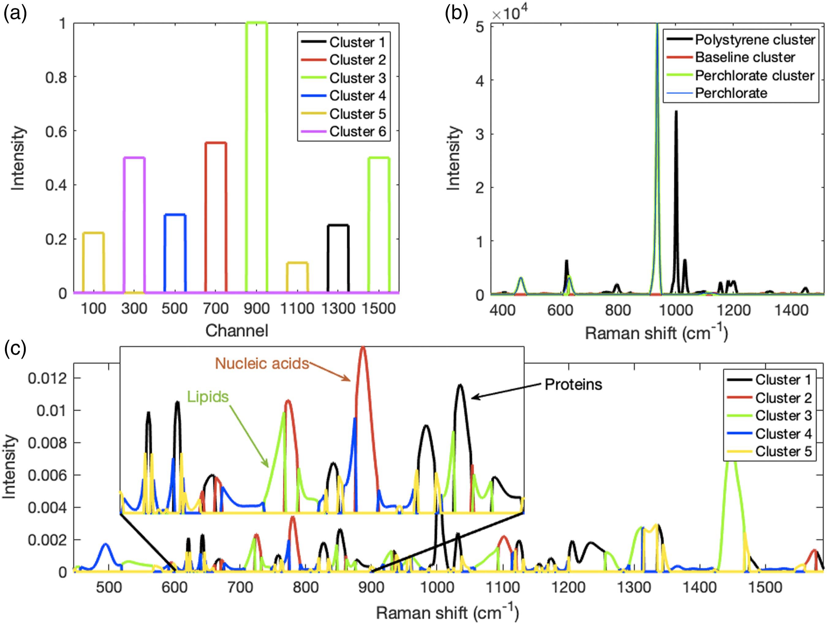
High correlations are also evident between proteins and nucleic acids, for example, between the 782 cm−1 composite nucleic acid peak and the 854 cm−1 composite protein peak indicated by the reddish square within the upper dotted circle in Fig. 5b. However, no corresponding cross-cluster is observed in Fig. 5d (upper dotted circle) because the clusters are exclusive: a profile cannot belong to two clusters simultaneously and hence a nucleic acid–protein cross-cluster cannot exist. However, contrary to 2D-COR, opposing or anticorrelated changes between peaks cannot be directly determined from 2D-CMS because they will simply be assigned to different clusters. Instead, opposing changes must be inferred from the profiles of their centroids in Fig. 5c. The anticorrelated change between declining lipid intensities (due to methanol-provoked lipid leaching) 32 and increasing nucleic acid intensities (possibly from nucleic acid precipitation) 51 can be determined for the 717 cm−1 phosphatidylcholine and 782 cm−1 composite nucleic acid 2D-COR cross-peak (solid circle in Fig. 5b) but not for 2D-CMS (solid circle in Fig. 5d) as there is no cross-cluster.
Overall, as for the 2D-CMS of synthetic data in Fig. 3d and model system data in Fig. 4d, the discrete nature of the 2D-CMS of measured Raman spectra permits a differential assessment of relationships between different Raman peaks that makes it complementary to 2D-COS while displaying greater sparsity than the corresponding 2D-COV and 2D-COR. The more complex example, indicated by the two bottom circles above 782 cm−1 and 827 cm−1 on the x-axis in Figs. 5b and 5d, will be discussed with the aid of Fig. 6.
Cluster-Segmented Spectra. Cluster-segmented spectra for the synthetic data are shown in Fig. 6a, for the model system Raman spectra in Fig. 6b and for the Jurkat cell Raman spectra in Fig. 6c. A cluster-segmented spectrum shows those channels or wavenumbers of a spectrum with profiles that belong to the same cluster, hence peaks belonging to the same cluster can be discerned. Though we have previously introduced and used cluster-segmented spectra to cluster spectroscopic with non-spectroscopic data,18,52 our objective was merely to group similar profiles together and not, as we do here, to segregate into groups with highly correlated yet qualitatively different profiles.
The cluster-segmented spectrum in Fig. 6a represents the same data (clusters and their color coding) as in Figs. 3c and 3d. Presenting the clustered information this way makes it easy to see which peaks belong to each profile cluster. 18 Thus, peaks at channels 100 and 1100 belong to the same cluster (yellow) as can be seen from the 100 × 1100 and 1100 × 100 cross-clusters in Fig. 3d because they have the same cluster profile that is shown in Fig. 3c. A similar argument applies to the green peaks at channels 900 and 1500 while the other color-coded peaks each belongs to separate clusters with different Fig. 3c profiles.
The model system contained only polystyrene and perchlorate and their peak intensities changed in opposite ways, thus their peaks belong to different clusters. Furthermore, except for two peaks near 600 cm−1, their peaks do not overlap. Consequently, their cluster-segmented spectra in Fig. 6b almost match the complete spectra of polystyrene and perchlorate. This is illustrated by imposing a scaled perchlorate spectrum on the cluster-segmented spectrum of the perchlorate ion.
In Fig. 6c we show with the same cluster colors the cluster-segmented mean spectrum of the Figs. 5c and 5d clustered profiles. All the wavenumbers belonging to the same cluster, hence the most qualitatively similar Fig. 5c profiles, are shown by the color of their cluster. The inset shows an expansion of the 600 to 900 cm−1 fingerprint spectral region that contains peaks from lipids (e.g., phosphatidylcholine at 717 cm−1), nucleic acids (e.g., composite peak at 782 and adenine at 725 cm−1), and proteins (e.g., composite peaks at 854, 827, 643, and 621 cm−1); thus, we assigned the green cluster to lipid peaks, the red cluster to nucleic acid peaks and the black cluster to protein peaks (see also Fig. 2c). Extending these assignments to the remainder of the spectrum showed fairly consistent labeling of macromolecular peaks. Other lipid peaks were labeled around 536 cm−1 (cholesterol ester), 1299 cm−1 (CH2 deformation in lipids), and 1446 cm−1 (various CH2 modes in lipids). Nucleic acid peaks were also labeled around 1099 cm−1 (phosphodioxy modes in nucleic acids) and 1573 cm−1 (ring breathing modes in nucleic acid bases). Additional protein peaks were identified around 758 and 887 cm−1 (tryptophan), 1003 and 1031 cm−1 (phenylalanine), and 1233 cm−1 (protein amide III modes).
Not all peaks were labeled in a clear manner. The Raman peak ∼720 cm−1 in cell and tissue spectra is a composite band due to the fusing of overlapping peaks from phosphatidylcholine (717 cm−1) and adenine (725 cm−1) and they were correctly clustered as shown by the partitioning of the peak into green (lipid) and red (nucleic acid) segments. Similar peak segmentations occur for other peaks consisting of overlapping bands from different macromolecules and these might be complicated. For example, both protein and nucleic acid bands occur near 667 cm−1 and the cluster-segmented spectrum for this region shows a central black protein peak flanked by two red nucleic acid segments. It is unclear whether the central black peak with red flanking segments should be interpreted as being due to a protein peak with distinct nucleic acid moieties on either side or whether a more intense and narrow protein peak is superimposed on a weaker but broader composite nucleic acid peak. Thus, a distinction must be made on the basis of prior information. Related to this, the reddish 2D-COR square in the lowest dashed circle in Fig. 5b seems to be partitioned into the corresponding two red cluster (nucleic acid) segments in the lowest dashed circle in Fig. 5d. The central part between these red cluster segments is missing but present as a black square in the adjacent dotted circle. Though the precise interpretation of the fragmented 667 cm−1 peak is unclear, this example demonstrates an important difference. It shows how the Fig. 5d 2D-CMS lowest circles provide a complementary interpretation of the same ones in the Fig. 5b 2D-COR by virtue of identifying peaks that are related due to having highly similar profiles as opposed to peaks that are related by virtue of being highly correlated.
Applying 2D-CMS might identify clusters with a large number of peaks. These peaks provide robust and unambiguous perturbation responses and so might be particularly useful in further analysis and interpretation. Clusters with few recognizable peaks might be of little use due to a somewhat random grouping of profiles degraded by overlapping neighbors, low abundance, or other effects. Thus, we have not been able to identify a carbohydrate or “other” cluster above.
Limitations. Though investigating in more depth is outside the scope of the current work, we mention several issues that complicate the utility of 2D-CMS. First, when used in the manner presented here, conformational changes in a given type of macromolecule might lead to peak shifts or intensity changes that would affect the profiles of the peaks involved. Thus, the profiles of some peaks of the same macromolecule might be assigned to one cluster while its other peak profiles might be assigned to a different cluster. This introduces complications, though such effects might in themselves offer opportunities for exploitation. For example, an analysis of the particular peaks assigned to two different clusters might provide insight into the nature of the conformational changes. An additional associated difficulty that emerges is the determination of the number of clusters to use in such a case to obtain meaningful results. Using more clusters might reveal more types of macromolecules, but it could also lead to more fragmented results in that overlapping peaks or other effects modify peak profiles enough to separate some peaks from their true clusters and group them with others to which they might be unrelated.
Second, individual lipids or proteins or nucleic acids could change independently in response to a perturbation. Though the exact cause is yet uncertain, this is hinted at by the ∼495 cm−1 DNA peak that was assigned to a different cluster (blue) from the cluster (red) to which the other nucleic acid peaks in Fig. 5d and Fig. S2d (Supplemental Material) were assigned. This creates both problems and opportunities, as mentioned above. Third, overlapping peaks that change in unrelated ways might sufficiently distort the profiles of associated wavenumbers to cause misclassification. It is possible that the 495 cm−1 DNA peak discussed above was assigned to cluster 4 due to the being affected by changes in the partly overlapping glycogen band around 485 cm−1. 53 Like many issues that arise in the case of overlapping peaks, this problem might not be tractable without enhancing the resolution of spectra. 54 A final difficulty relates to the selection and back addition of constant profiles in a manner that effectively segregates them from the constant profiles of baseline wavenumbers. Though the smoothing of spectra can suppress noise, 55 residual noise will be present in such profiles, and this will be accentuated through division by their standard deviations. One possibility might be to use the square root relationship between Poisson noise and signal intensity. 55 For example, to be considered a constant profile, the mean profile intensity has to exceed the LOD, its noise distribution has to be approximately Gaussian and the noise level (i.e., the profile standard deviation) must be less than the square root of the mean peak intensity.
Conclusion
The interpretation of two-dimensional correlation spectra from many types of biomedical, pharmaceutical, or microbiological samples is often not a straightforward task due to their high complexity. 56 With 2D-CMS, we used k-means clustering to group the wavenumber profiles of Raman hyperspectra into discrete classes and constructed sparse two-dimensional cluster member spectra and cluster-segmented spectra to complement 2D-COS. 2D-COS maps present Raman hyperspectral data in a manner where variances and correlation coefficients between Raman peaks generally change in a continuous manner, where peak intensity changes in opposite directions can be visualized because they manifest as negative cross-peaks and where numerous cross-peaks exist even between unrelated peaks. 2D-CMS provides complementary information. It presents hyperspectral data in a discrete manner showing only peaks whose changes are highly similar and thus belong to the same cluster. Peak intensity changes that are dissimilar are shown in different clusters; hence, cross-clusters (analogous to 2D-COS cross-peaks) do not exist. Peak intensity changes in opposite directions also cannot be represented because opposing peak intensity changes will be assigned to different clusters. These attributes make 2D-CMS simpler in appearance than 2D-COS maps. The partitioning of peak intensity changes into meaningful categories also makes them easy to visualize. Ease of visualization is further supported by cluster-segmented spectra where the peaks or peak segments (due to overlapping peaks) in a spectrum are colored according to their cluster. We have applied 2D-CMS to synthetic spectra, Raman spectra from a model system and from highly complex mammalian cell spectra and successfully shown how 2D-CMS facilitates the identification of related peaks using cluster-based as opposed to correlation-based similarities. Thus, we expect that this approach might be useful on its own as well as aid in the interpretation of the plethora of auto and cross-peaks with different amplitudes and signs that are present in two-dimensional correlation spectra.
Supplemental Material
sj-pdf-1-asp-10.1177_00037028221133851 - Supplemental material for Two-Dimensional Clustering of Spectral Changes for the Interpretation of Raman Hyperspectra
Supplemental Material, sj-pdf-1-asp-10.1177_00037028221133851 for Two-Dimensional Clustering of Spectral Changes for the Interpretation of Raman Hyperspectra by H G. Schulze, Shreyas Rangan, Martha Z. Vardaki, Michael W. Blades, Robin F. B. Turner, and James M. Piret in Applied Spectroscopy
Footnotes
Acknowledgments
The authors thank Riley Wong for help with collecting and preprocessing spectra. We also acknowledge the Canadian Foundation for Innovation and the British Columbia Knowledge Development Fund for funding the purchase of instrumentation made available for this work through the UBC Laboratory for Molecular Biophysics.
Declaration of Conflicting Interests
The author(s) declared no potential conflicts of interest with respect to the research, authorship, and/or publication of this article.
Funding
The author(s) disclosed receipt of the following financial support for the research, authorship, and/or publication of this article: This work was supported by the Natural Sciences and Engineering Research Council of Canada and the Canadian Institutes of Health Research.
Supplemental Material
All supplemental material mentioned in the text is available in the online version of the journal.
References
Supplementary Material
Please find the following supplemental material available below.
For Open Access articles published under a Creative Commons License, all supplemental material carries the same license as the article it is associated with.
For non-Open Access articles published, all supplemental material carries a non-exclusive license, and permission requests for re-use of supplemental material or any part of supplemental material shall be sent directly to the copyright owner as specified in the copyright notice associated with the article.