Sage Journals: Discover world-class research

Abstract

Whereas postmortem ischemic damage is common in head injury, antemortem demonstration of ischemia has proven to be elusive. Although ¹⁵O positron emission tomography may be useful in this area, the technique has traditionally analyzed data within regions of interest (ROIs) to improve statistical accuracy. In head injury, such techniques are limited because of the lack of a priori knowledge regarding the location of ischemia, coexistence of hyperaemia, and difficulty in defining ischemic cerebral blood flow (CBF) and cerebral oxygen metabolism (CMRO2) levels. We report a novel method for defining disease pathophysiology following head injury. Voxel-based approaches are used to define the distribution of oxygen extraction fraction (OEF) across the entire brain; the standard deviation of this distribution provides a measure of the variability of OEF. These data are also used to integrate voxels above a threshold OEF value to produce an ROI based upon coherent physiology rather than spatial contiguity (the ischemic brain volume; IBV). However, such approaches may suffer from poor statistical accuracy, particularly in regions with low blood flow. The magnitude of these errors has been assessed in modeling experiments using the Hoffman brain phantom and modified control datasets. We conclude that this technique is a valid and useful tool for quantifying ischemic burden after traumatic brain injury.

Keywords

Trauma Head injury Positron emission tomography Cerebral ischemia Ischemic penumbra

Commonly quoted CBF and CMRO2 thresholds for neuronal survival based upon oxygen-15 positron emission tomography (¹⁵O PET) studies of experimental ischemia and clinical stroke (Heiss et al., 1992; Marchal et al., 1996; Powers et al., 1985) cannot be translated directly to head injury. A depressed level of consciousness, therapeutic sedation, and trauma-induced mitochondrial dysfunction (Verweij et al., 2000) can reduce metabolic rate (and hence coupled perfusion) in the injured brain and reduce critical CBF thresholds for ischemia (Bergsneider et al., 2000). Conversely, epileptiform activity, or hypermetabolism associated with excitotoxicity, may increase CMRO2 and make “normal” CBF levels inadequate. A clear definition of ischemia in situations where CMRO2 is altered depends upon the demonstration of compensatory increases in oxygen extraction fraction (OEF). Such data from patients with head injury in the PET literature are sparse and limited by methodologic difficulties (Diringer et al., 2000, 2002). Furthermore, even if such thresholds can be defined, their application to parametric PET images obtained in head injury may require methodologic adaptation. Ischemia in stroke usually conforms to topographical patterns, with identification of an ischemic core and penumbra (Baron, 1999). Whereas ischemia may be prominent in perilesional areas in head injury (Bouma et al., 1992; McLaughlin and Marion, 1996), significant ischemia may also be observed in structurally normal brain (Coles et al., 2002b). Consequently, a method is needed that can estimate the burden of critical hypoperfusion and ischemia across the entire brain, making no assumptions regarding its location. Such an approach requires definition of tissue with evidence of “misery perfusion” based upon individual voxel measurements and construction of a region of interest (ROI) based upon physiology rather than spatial contiguity. This voxel-based approach has clear methodologic pitfalls. It is highly dependent upon the statistical accuracy of the PET methods used and the underlying signal to noise characteristics of the PET data (Lammertsma et al., 1982). Such concerns are particularly relevant in disease states such as head injury where acute reductions in blood flow are likely. The reduction in emission counts within regions of the brain with low blood flow compromises the statistical accuracy of the technique.

The aim of this report is to quantify some of the methodologic problems of voxel-based summary measures of ischemia using ¹⁵O PET. We have used control and phantom data sets to explore the confidence with which differences in voxel-based measurements of ischemic burden can be ascribed to real physiologic changes in the presence of emission data of varying statistical quality.

METHODS

To illustrate the difficulties in the selection and interpretation of ROI based analyses and the benefits of a voxel-based approach in head injury, we present results from two patient data sets and a typical control. To assess the effect of a reduction in emission counts, and by inference statistical accuracy, upon voxel-based measurements of ischemia and critical hypoperfusion, we have used a range of different methods. First, we obtained tracer concentrations from clinical studies and used these figures as a basis for producing realistic phantom data sets. Second, control data sets were manipulated by varying the duration of emission acquisition to model a reduction in statistical accuracy. Third, data were collected from the Hoffman brain phantom (Hoffman et al., 1990) using the tracer concentrations obtained from clinical studies to produce clinically relevant phantom data sets. We varied tracer concentrations (and hence the signal to noise) in these experiments while keeping physiologic parameters (CBF, CMRO2, and OEF) unchanged. Data collected using these methods were used to assess the effect of a reduction in signal-to-noise upon voxel-based measurements of ischemia. Finally, we investigated the effect of changes in the small-to-large vessel hematocrit ratio (R), blood-brain partition coefficient for H₂ ¹⁵O (ρ), and signal-to-noise in C¹⁵O emission data using simulations.

Data acquisition

All PET studies were undertaken on a General Electric Advance scanner (GE Medical Systems, Milwaukee, U.S.A.).

Clinical ¹⁵O PET studies. To model the effect of changes in image statistics on summary measurements of brain ischemia and obtain tracer concentrations for use in generating realistic phantom datasets, we examined ¹⁵O PET datasets obtained from 10 healthy volunteers (8 male, 2 female) and 12 patients within 24 hours of head injury (10 male, 2 female). The mean (range) age of controls and patients was 30 (18–60) years and 39 (16–70), respectively. All patients sustained a severe or moderate head injury (Glasgow Coma Score (GCS) ≥ 8, and 9–12 respectively) with secondary neurologic deterioration requiring sedation and control of ventilation. All volunteers provided informed consent for studies, and assent was obtained from the next of kin for all patient studies. All studies were approved by the Local Research Ethics Committee at Addenbrooke's Hospital, Cambridge, UK, and by the Administration of Radioactive Substances Advisory Committee of the UK.

Emission data were acquired in 3D mode during a 20-minute steady state infusion of 800 MBq of H₂ ¹⁵O (two 5-minute frames at the end of the administration), following a 60-second inhalation of 300 MBq of C¹⁵O (single 5 minute frame), and in 2D mode during a 20-minute steady state inhalation of 7200 MBq of ¹⁵O₂ (two 5-minute frames at the end of the administration). Just before emission data acquisition, a 10-minute transmission scan was performed using rotating germanium, 68 rods (2 × 300 MBq). This data, in combination with that from a 60-minute blank scan acquired on the same day, was used to correct the emission data for photon attenuation.

Control data with reduced acquisition time

One way to assess the impact of a reduction in image statistics on voxel-based measurements of ischemia is to reduce emission counts in control data to simulate the effect of a reduction in CBF. The 10-minute emission data from H₂ ¹⁵O and ¹⁵O₂ scans were acquired in at least two 5-minute frames in all subjects and in four 2.5-minute frames in six of the control subjects. We therefore recalculated the control data using 25% and 75% of the emission data (using one or three of the four 2.5-minute frames respectively) in the six control subjects for whom data was available in this format and using 50% of the emission data (using two of four 2.5-minute frames or one of two 5-minute frames) in all 10 controls. These reductions in acquisition time simulate the counts acquired within a 10-minute acquisition but with reduced tracer concentration (C_t). The effective reduction in C_t for 25%, 50%, and 75% of the emission data is related to CBF through the steady state equation (Frackowiak et al., 1980),

CBF = \frac{λ}{(C_{a} / C_{t} - (1 / ρ)}

(1)

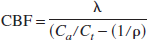
where Λ is the decay constant for ¹⁵O, and C_a is the arterial tracer concentration.

Consequently, these reductions in acquisition time result in images with statistical quality corresponding to a global CBF of 5.0, 11.7, and 21.5 mL·100g⁻¹·min⁻¹ respectively, compared with a baseline value in controls of 37 mL·100g⁻¹·min⁻¹. These analyses would therefore simulate the effect of a CBF of approximately 5, 10, and 20 mL·100g⁻¹·min⁻¹ without any change in physiology (Lammertsma et al., 1982).

Hoffman ¹⁸F phantom studies

Emission data were acquired sequentially in 2D and 3D modes as the radioactivity in the phantom decayed from an initial 150 MBq of ¹⁸F-fluoride. A series of 2 × 5-minute emission frames were obtained in each acquisition mode over a range of count rates that encompassed those from patient and control ¹⁵O₂ and H₂ ¹⁵O scans. Emission data were corrected for photon attenuation using two combinations of transmission and blank scans: 10-minute transmission and 1-hour blank (as used for clinical data); 2-hour transmission and 2-hour blank (to minimize any noise propagation from the attenuation correction).

Image reconstruction and kinetic modeling

Images were reconstructed into 2.34 × 2.34 × 4.25 mm voxels using the PROMIS 3D filtered back projection algorithm (Kinahan and Rogers, 1989), with corrections applied for attenuation, scatter, randoms, and dead time. During reconstruction, a Hanning filter cutoff at the Nyquist frequency was used transaxially, but no apodisation was applied axially. Emission images were then smoothed using an isotropic 4 mm Gaussian filter. Parametric maps of CBF, CBV, CMRO2, and OEF were calculated by inputting PET emission and arterial tracer activity measurements into standard models (Frackowiak et al., 1980; Lammertsma et al., 1987) implemented in custom designed software (PETAN) (Smielewski et al., 2003). We used a blood-brain partition coefficient for H₂ ¹⁵O (ρ) of 0.95 based upon previous in vitro data (Herscovitch and Raichle, 1985) and a small-to-large vessel hematocrit ratio (R) of 0.85 (Phelps et al., 1979). Parametric maps were coregistered to anatomy using magnetic resonance (MR) imaging in phantom and control studies and x-ray computed tomography (CT) in patients.

Generation of parametric maps from Hoffman phantom data.

To generate images that mimicked the heterogeneous pattern of OEF within the injured brain, we constructed an ROI map (Fig 1) consisting of five ROIs with differing physiology. These ROIs were irregular in shape and spatial distribution so as to mimic the spatially heterogeneous pattern of pathophysiology observed in patients (Coles et al., 2002b). We defined the physiology in these ROIs as follows: first, we rearranged Equation 1

C_{t} = \frac{C_{a}}{(λ / CBF) + (1 / ρ)}

(2)

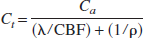
to select 3D phantom data (which simulated H₂ ¹⁵O scans) with average C_t values corresponding to a range of clinically relevant CBF values. The CBF values chosen (28, 31, 34, 38, and 43 mL·100g⁻¹·min⁻¹) ranged around the mean CBF obtained in patients (34 mL·100g⁻¹·min⁻¹). Each CBF value was attributed to one of the regions in the ROI map. To vary the image statistics within a clinically relevant range, C_t values in each region were calculated for six different arterial tracer activity inputs (C_a). The C_a values used were those observed in the average patient (AP), worst patient (WP), and best patient (BP), and the average control (AC), worst control (WC), and best control (BC).

Next, for each CBF and C_a value, once the required C_t for the ROI was determined, we calculated the tissue tracer concentration required in the 2D phantom data (which simulated the ¹⁵O₂ scans) to achieve a range of OEF values using the standard equation for OEF (Frackowiak et al., 1980). The 2D emission frames chosen for each region were selected to maintain unchanged CMRO2 and result in OEF values of 60, 55, 50, 45, and 40% within the respective ROIs (Fig. 1).

Fig. 1.

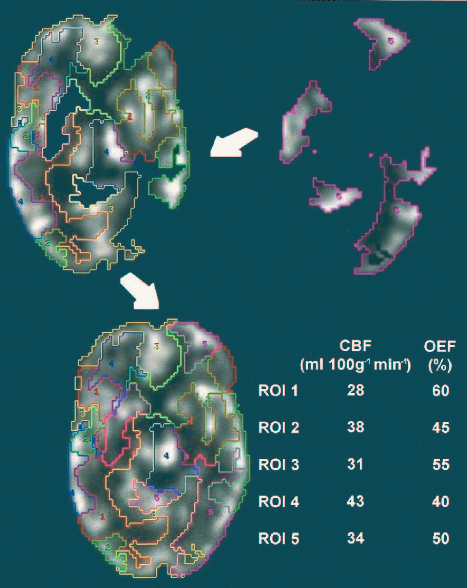
Construction of parametric maps for the phantom data sets. These ROI were designed to cover the whole brain and include mixed regions of grey and white matter and cerebrospinal fluid. For each of the clinical scenarios and reference data sets, the composite emission images for H₂ ¹⁵O and ¹⁵O₂ were created using regions selected from appropriate 3D and 2D emission frames respectively. Each data set was processed to produce CBF, CMRO2, and OEF maps with identical physiology but varying statistical accuracy. ROI, regions of interest; OEF, oxygen extraction fraction.

As the phantom data did not have tracer concentrations that exactly matched those calculated from the CBF and OEF equations, the 3D and 2D data selected for the regions were scaled (average correction 6 ± 3%). This ensured that the regional and global CBF, CMRO2, and OEF were unchanged, with global values comparable with those obtained in a typical patient (CBF 34 mL·100g⁻¹·min⁻¹, CMRO2 2.4 mL·100g⁻¹·min⁻¹, and OEF 50%). Whereas the regional and global physiology in each of these composite data sets was identical, the varying tissue tracer concentrations resulted in varying image statistics.

We defined two additional data sets as points of reference at the two ends of the spectrum of statistical accuracy. These were well outside the range of data sets that we obtained in clinical practice. First, the emission frames with the lowest counts were used to represent the worst ¹⁵O₂ and H₂ ¹⁵O emission frames. Second, for both 2D and 3D acquisitions, a weighted sum was made from all the frames, which was reconstructed using the 2-hour transmission and blank scans to generate emission frames with the optimal signal-to-noise ratio characteristics. These two were labeled the worst reference (WR) and best reference (BR) data sets, respectively. For the worst and best image data sets, arterial tracer activity measurements equivalent to those for the average patient were used, and the five regions were scaled appropriately to maintain CBF, CMRO2, and OEF. Thus all eight data sets represented images of the same virtual physiology (with identical values of CBF, CMRO2, and OEF) but varied in statistical accuracy from extremely poor (WR) to optimal (BR) through the various clinical scenarios modeled (AP, WP, BP, AC, WC, and BC) (Fig. 1).

Image analysis

Voxel-based analysis. Ischemic brain volume. We used OEF to assess the burden of ischemia in PET images to avoid the confounding effects of drug- and injury-induced metabolic suppression on CBF and CMRO2. Individual anatomic images were edited to extract a template that identified brain tissue voxels and excluded extracranial tissue, cerebrospinal fluid, and extra-axial hematomas. This brain template was applied to coregistered parametric PET images to generate frequency histograms of OEF. From these data, we sought to define a critical threshold for OEF likely to result in tissue damage if sustained. It is difficult to find data that identify critical increases in OEF levels that still allow survival in the setting of ischemia, but some guidance is available from both human (Powers et al., 1985; Yundt and Diringer, 1997) and experimental data (Sutton et al., 1990). Sutton et al. (1990) identified the cerebral venous oxygen content (CvO₂) as the critical predictor of infarction in experimental ischemia, with the highest observed CvO₂ threshold for infarction being 2.9 mL/100 mL. Clinical studies (Powers et al., 1985; Yundt and Diringer, 1997) are broadly concordant with these data and suggest that brain regions can survive in the setting of prolonged ischemia with local CvO₂ levels as low as 3.5 mL/100 mL. Consequently, we estimated an individualized critical OEF threshold (OEF_crit; which equated to a CvO₂ of 3.5 mL/100 mL) for each subject as follows:

{OEF}_{crit} = \frac{(C_{a} O_{2} - 3.5)}{C_{a} O_{2}}

(3)

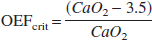
where CaO₂ is arterial oxygen content calculated as (1.34 ϗ Hb ϗ (SaO₂/100)) + (0.003 ϗ PaO₂), Hb = hemoglobin in g/100 mL, SaO₂ = arterial oxygen saturation (%). Application of these thresholds to OEF images allowed us to calculate the volume of voxels with CvO₂ values below this threshold and hence allowed estimation of the ischemic brain volume (IBV) (Fig. 2).

Fig. 2.

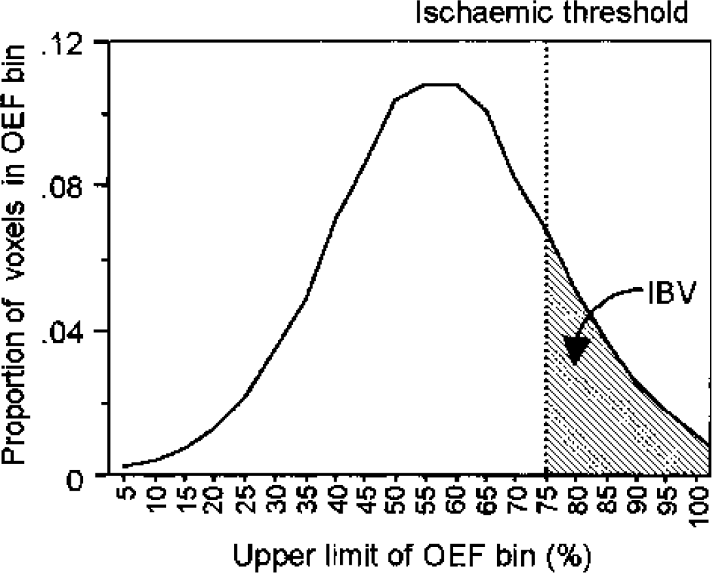
Calculation of the ischemic brain volume. OEF histogram from a single patient, showing the distribution of the number of voxels in each OEF bin. Critical OEF thresholds are derived by calculation of the OEF value above which cerebral venous oxygen content (CvO₂) would be less than 3.5 mL/100 mL. The summed volume of voxels with OEF values above this threshold is the IBV. OEF, oxygen extraction fraction; IBV, ischemic brain volume.

Perfusion-utilization matching. OEF values should be closely clustered in normal subjects, suggesting efficient matching of CBF to CMRO2, with a resulting narrow spread of OEF values (Lebrun-Grandie et al., 1983). We assessed the matching of oxygen supply to demand by inspection of the OEF histograms and measurement of the standard deviation of the distribution.

ROI and voxel-based analyses in illustrative clinical data sets. We have used a sample patient data set to illustrate the technique that we used to define perilesional ROIs for analysis: a region of interest map overlying the region of structural injury was drawn on the structural CT image, based upon the entire volume of cerebral tissue within 15 to 20 mm of the subdural hematoma (Fig. 3A). It is extremely difficult to identify the extent of tissue injury using CT imaging alone. Because perilesional regions with CT evidence of edema demonstrate similar physiology to that found within normal appearing perilesional regions (Steiner et al., 2003), we defined such ROIs based upon distance from lesion, rather than CT appearance. The structural ROI identified in Fig. 3 incorporates the volume of brain tissue in close proximity to the primary injury and likely to demonstrate the greatest physiologic derangement. Physiologic parameters were expressed as an average for all brain tissue within the ROI. Both CT and PET images obtained in patients provide poor grey-white matter discrimination, making it impossible to accurately segment anatomic areas and derive appropriately weighted averages for CBF and CMRO2. Consequently, unweighted mean data values were obtained while recognizing that the effect of tissue heterogeneity on PET models would result in falsely low CBF and CMRO2 values (Baron et al., 1989; Correia et al., 1985; Herscovitch and Raichle, 1983). In addition, the illustrative patient and control data sets were used to show how the IBV and OEF distributions might differ in patients after head injury.

Fig. 3.

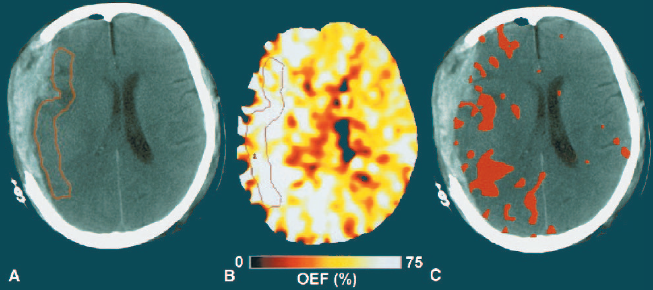
ROI and voxel-based analysis of a patient within 24 hours of head injury. (A) x-ray CT obtained from a 42-year-old woman 16 hours after injury following evacuation of a subdural hematoma. Note the small amount of residual subdural blood with minimal midline shift. A perilesional ROI has been drawn on the entire volume of cerebral tissue within 15 to 20 mm of the subdural hematoma. A single slice is shown here for simplicity. (B) OEF PET image. Note the marked increases in OEF in large portions of the cerebral hemisphere underlying the evacuated subdural hematoma. (C) x-ray CT with those voxels with OEF > 75% (based on a calculated CvO₂ < 3.5 mL/100 mL) shown in red. The full extent of the physiologic lesion is greater than can be immediately defined by examination of the structural CT image alone. CT, computed tomography; ROI, regions of interest; OEF, oxygen extraction fraction; PET, positron emission tomography.

Assessment of signal-to-noise characteristics as a confounder in voxel-based analyses. Control data with reduced acquisition time. The calculated IBV and measured SD of the OEF histograms of the control data sets with image statistics corresponding to a global CBF of 5.0, 11.7, and 21.5 mL·100g⁻¹·min⁻¹ were compared with values obtained from the undegraded control data sets.

Phantom data. To examine the effect of emission data signal-to-noise characteristics on the IBV and SD of the OEF histograms the phantom data modeling the different clinical scenarios and reference phantom data sets were compared.

Assessment of the effect of the small-to-large vessel hematocrit ratio and blood-brain partition coefficient (ρ) for H₂ ¹⁵O upon OEF measurement. In this paper we have used OEF images, calculated using fixed values for small-to-large vessel hematocrit ratio (R) and ρ, to define disease pathophysiology after head injury. It is important to recognize that regional variations in such constants are highly likely after trauma, and the impact of such effects upon the OEF calculation should be considered. Because the correction for intravascular ¹⁵O₂ used in this paper to calculate the OEF parametric images is independent of the value of R (Lammertsma et al., 1987), the choice of value for this constant will have no impact upon the data and conclusions of this study.

To model the effect of variation in the value for ρ upon OEF and voxel-based measures of ischemia, we used the arterial tracer concentration of the average patient within 24 hours of head injury and variable tissue tracer concentrations to construct data with a range of OEF values (20%, 40%, 60%, and 80%). In these simulations, the CMRO2 and CBV remained constant and comparable to the typical values obtained in a patient (2.4 and 4.2 mL·100g⁻¹·min⁻¹, respectively), and changes in OEF were achieved by varying CBF from a baseline value of 34 mL·100g⁻¹·min⁻¹. In each case the effect of a change in the value of ρ upon the calculated OEF was assessed.

Assessment of C¹⁵O signal-to-noise characteristics upon the measurement of OEF. A further source of potential error concerns the signal-to-noise characteristics of the C¹⁵O emission data. Because the correction for intravascular ¹⁵O₂ within the OEF calculation is dependent upon the CBV (Lammertsma et al., 1987), any error within the CBV measurement will be propagated within the OEF calculation. The concern is that OEF values within injured brain regions may be increased to potentially ischemic levels because of poor signal-to-noise within the C¹⁵O emission data. To model the effect of CBV upon OEF, we defined the distribution of CBV values seen in our patient data sets. This range of CBV values included those caused by noise. We then modeled the effect of change in CBV over this range on the OEF data described in the previous section. This provided an estimate of the impact of changes in OEF attributable to errors in CBV measurement in clinical data sets.

Statistical analysis

Statistical analysis was undertaken using Statview (Version 5, 1998, SAS Institute Inc., Cary, NC, U.S.A.). All data are expressed and displayed as mean ± SD unless otherwise stated. Voxel-based PET data from the modified control data were compared using two-tailed paired t-tests. P values of < 0.05 were considered significant.

RESULTS

ROI and voxel-based analyses in illustrative clinical data sets

In Fig. 3, the results of a perilesional ROI based upon structural imaging are compared with that of a voxel-based analysis technique. Although the ROI data are suggestive of compromised tissue (CBF 15 mL·100g⁻¹·min⁻¹, CBV 3.3 mL·100g⁻¹, CMRO2 1.6 mL·100g⁻¹·min⁻¹, and OEF 65%), they are not conclusive. In fact, the ROI fails to capture the entire physiologic injury, whereas the voxel-based technique generated from those voxels with a calculated CvO₂ of < 3.5 mL/100 mL suggests that large portions of the cortex ipsilateral to the lesion are at risk of ischemic damage and neuronal loss, with a calculated IBV of 92 mL. In comparison with a typical control data set, the OEF histogram from this patient is broader and shifted to the right with a standard deviation of 25.7% versus 9.3% (Fig. 4A). In Fig. 4B, the OEF distribution of a second patient data set shows greater variability with regions of both high OEF suggestive of ischemia and low OEF suggestive of hyperemia or neuronal dysfunction (SD 17.6%). This suggests a more generalized impaired coupling of flow and metabolism, rather than classical regional ischemia.

Fig. 4.

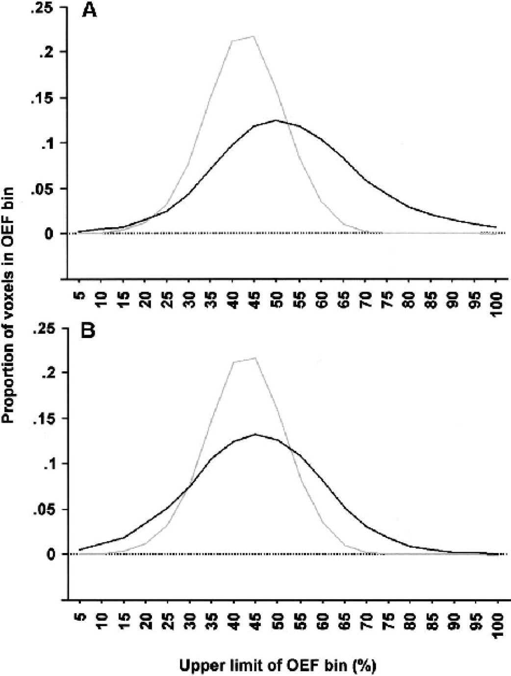
Comparison of patient and control OEF histogram distributions. OEF histograms from a volunteer (grey) and two representative patients within 24 hours of injury (black). (A) The patient histogram is broader and shifted to the right, with a prominent ischemic “tail” composed of voxels with high OEF values. (B) The patient histogram is broader with regions of both high and low OEF suggestive of ischemia and hyperemia respectively. OEF, oxygen extraction fraction.

Emission tracer concentrations in patient and control acquisitions

Mean tracer concentrations in control and patient data sets were similar. Control subjects showed mean (range) tracer concentrations of 6.1(3.4 to 8.1 kBq/mL) for ¹⁵O₂ and 3.8 (2.5 to 5.4 kBq/mL) for H₂ ¹⁵O. Mean (range) tracer concentrations in patients were 8.6 (5.1 to 13) for ¹⁵O₂ and 4.4 (3.1 to 7 kBq/mL) for H₂ ¹⁵O. In addition to inter-subject variability, there were clearly significant variations in tracer concentrations across the brain within subjects, and particularly within patients. However, voxels with extremely low emission counts represented a very small fraction of the brain volume. The highest volume of brain tissue in any patient with emission counts consistent with a CBF < 10 mL·100g⁻¹·min⁻¹ was 72 mL (6.5% of the brain volume) and less than one third of these voxels showed high OEF (based upon a calculated CvO₂ of < 3.5 mL/100 mL) (22 mL or approximately 2% of the brain volume). Similarly, the highest volume of brain tissue with emission counts consistent with a CBF less than 5 mL·100g⁻¹·min⁻¹ was 32 mL (3% of the brain volume), but voxels with a CBF < 5 mL·100g⁻¹·min⁻¹ coupled with high OEF comprised, at most, 11 mL (representing approximately 1% of the brain volume).

Assessment of signal-to-noise characteristics as a confounder in voxel-based analyses

Control data with reduced acquisition time. The statistical accuracy of the control data was degraded by a reduction in the duration of emission frame acquisition. This resulted in images with noise levels corresponding to a mean CBF of approximately 20, 10, and 5 mL·100g⁻¹·min⁻¹ (compared with a mean CBF of 37 mL·100g⁻¹·min⁻¹ in the complete data sets) and was achieved using control data with 75%, 50%, and 25% of the total emission frame duration, respectively. These changes in image statistics produced statistically significant increases in IBV in the control data sets (P < 0.05 for all comparisons; paired t-tests) (Fig. 5A). However, the absolute increases in ischemic brain volume were relatively small, except with the most severe degradation in image statistics (increases of 1.5 ± 1.2, 9.4 ± 7.2 and 44.8 ± 31.6 mL, from a baseline value of 2.0 ± 3.4 mL in the complete control data sets). These increases can be viewed in the context of the IBV in the first patient data set (92 mL).

Fig. 5.

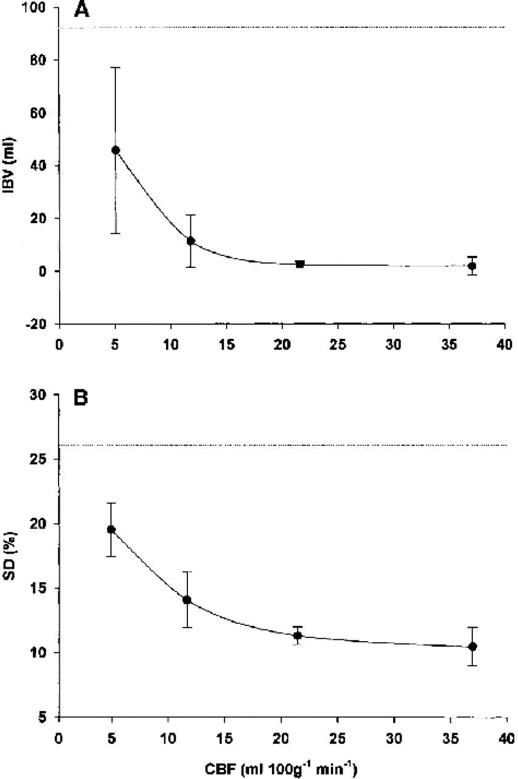
Simulated effects of a reduction in blood flow on control data. Control data reconstructed with 75%, 50%, and 25% of the total emission frame duration to simulate images with a blood flow of approximately 20, 10, and 5 mL·100g⁻¹·min⁻¹, respectively. Baseline data had a CBF of 37 mL·100g⁻¹·min⁻¹. (A) Mean ± SD curve to demonstrate the simulated effect of a reduction in global blood flow on the IBV. The IBV of the first reference patient data set is shown by the dotted line (92 mL). (B) Mean ± SD curve to demonstrate the simulated effect of a reduction in global blood flow on the SD of the OEF histogram. The SD of the OEF histogram of the first reference patient dataset is shown by the dotted line (26%). IBV, ischemic brain volume; SD, standard deviation; OEF, oxygen extraction fraction.

The degradation in image statistics also produced significant increases in the SD of OEF histograms at all stages (P < 0.001; paired t-tests). However, as with the IBV measurements, the absolute increases were relatively modest, except with the most severe degradation in image statistics (Fig. 5B).

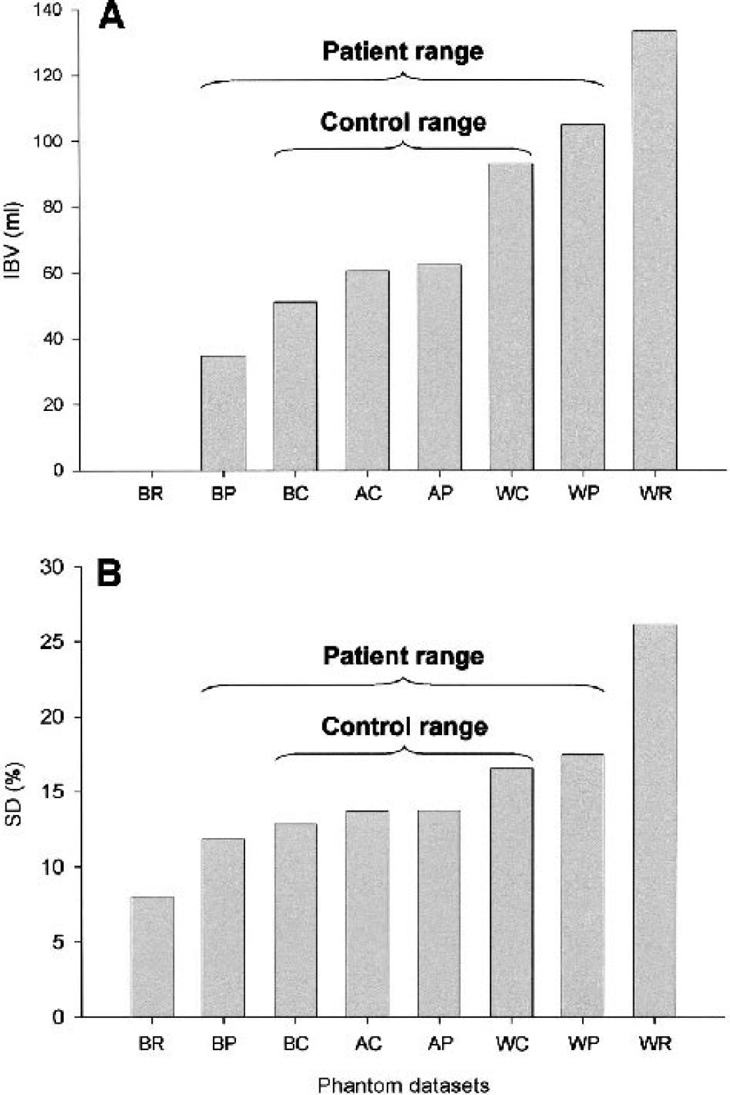
Phantom data. The data for the calculated IBV and SD of the OEF histograms for the different phantom data sets are displayed in Figs. 6A and 6B. As the tracer concentration, and hence counts, is reduced there is an increase in the calculated IBV and SD of the OEF histograms. Data sets with tracer concentrations identical to the average patient and control data sets (AP and AC) showed near identical values of IBV and SD of the OEF histograms. In addition, the values of IBV and SD of OEF histograms derived using the range of tracer concentrations from patients and controls showed complete overlap.

Fig. 6.

The effect of varying tracer concentrations in phantom data sets. (A) Histogram to demonstrate the calculated IBV of the worst and best reference data sets (WR and BR, respectively), and the best, worst, and average control and patient-simulated data sets (BC, WC, AC, BP, WP, and AP, respectively). (B) Histogram to demonstrate the measured SD of the OEF distribution for the worst and best reference data sets (WR and BR respectively), and the best, worst, and average control and patient-simulated data sets (BC, WC, AC, BP, WP, and AP, respectively). IBV, ischemic brain volume; SD< standard deviation; OEF, oxygen extraction fraction.

Assessment of the effect of the blood-brain partition coefficient (ρ) for H₂ ¹⁵O and C¹⁵O signal-to-noise characteristics upon OEF measurement

In Fig. 7, the effect of a change in the value for ρ on the measured OEF is displayed for a range of OEF values. As the value of ρ decreases, there is an increase in the calculated OEF value, particularly for regions with low OEF. Regions of the brain with high OEF appear least sensitive to such errors, with clinically significant increases in OEF only occurring with values for ρ of < 0.4.

In Fig. 8A, the effect of CBV on the calculated OEF is displayed for a range of OEF values. As the CBV value decreases below the baseline value of 4.2 mL·100g⁻¹, there is an increase in the calculated OEF value, particularly for CBV values below zero and within brain regions with low OEF. In Fig. 8B, the CBV histograms of the 12 patients following head injury are shown. The mean (range) volume of brain with CBV values less than zero was 4.7 (0.5 to 19.8) mL. These data show that, within the range of CBV values seen in our patient data sets, the impact of CBV on OEF calculation is small, particularly for high OEF values.

Fig. 8.

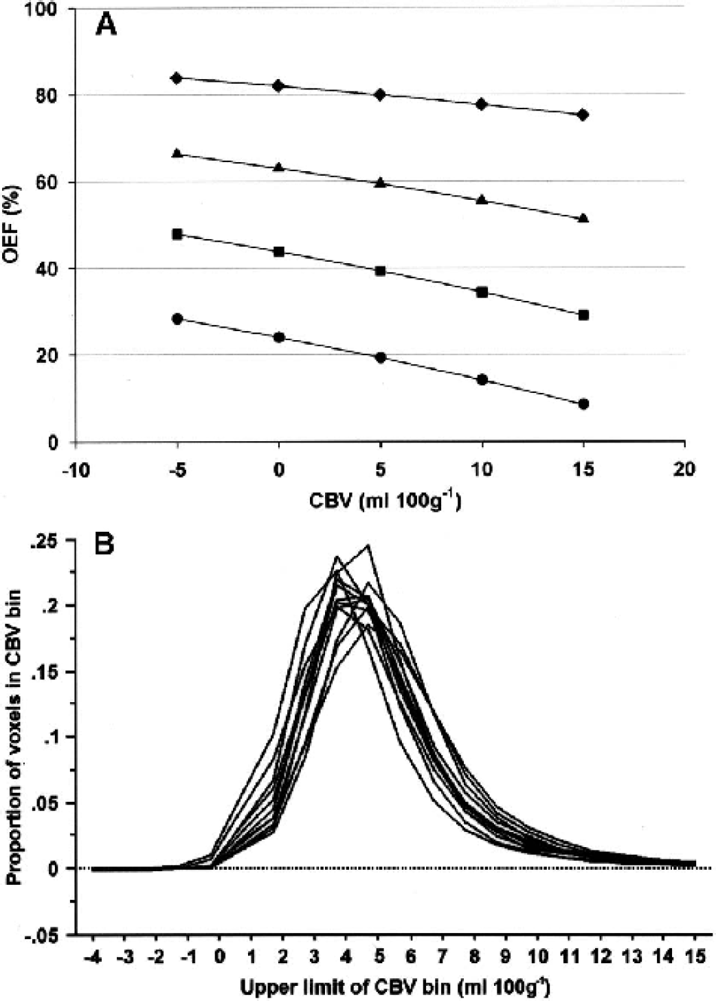
Assessment of the effect of CBV upon OEF measurement within the range of values seen in clinical data sets. (A) Curve to demonstrate the effect of CBV upon simulated patient data with OEF values of 20% (•), 40% (□), 60% (▲), and 80% (♦). In these simulations, the CMRO2 remained constant (2.4 mL·100g⁻¹·min⁻¹), and changes in OEF were achieved by varying CBF from a baseline value of 34 mL·100g⁻¹·min⁻¹. In each case, the effect of CBV upon the calculated OEF was assessed using the baseline CBV of 4.2 mL·100g⁻¹ and the range of voxel values obtained from 12 patients within 24 hours of head injury. (B) CBV histograms from 12 patients within 24 hours of injury, showing the distribution of voxels in each CBV bin. OEF, oxygen extraction fraction.

Fig. 7.

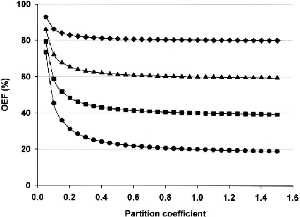
Assessment of the effect of the blood-brain partition coefficient for H₂ ¹⁵O upon OEF measurement. Curve to demonstrate the effect of a change in the value for the partition coefficient for H₂ ¹⁵O upon simulated patient data with OEF values of 20% (•), 40% (□), 60% (Δ), and 80% (♦). In these simulations, the CMRO2 and CBV remained constant (2.4 mL·100g⁻¹·min⁻¹ and 4.2 mL·100g⁻¹, respectively), and changes in OEF were achieved by varying CBF from a baseline value of 34 mL·100g⁻¹·min⁻¹. OEF, oxygen extraction fraction.

DISCUSSION

The purpose of this report was to explore the confidence with which differences in ischemic burden can be ascribed to physiologic changes for PET data of variable statistical quality. We found that the deterioration in image statistics from a simulated reduction in CBF resulted in statistically significant increases in the calculated IBV and SD of OEF histograms. However, the absolute changes in IBV and SD of OEF attributable to this methodologic manipulation were small and clinically insignificant in the context of actual IBV values that we have obtained in patients with severe head injury (Coles et al., 2002a).

It is important to define valid voxel-based methods for assessment of ischemic burden in this patient group. Conventional functional imaging approaches in clinical and experimental stroke have traditionally used CBF thresholds for ischemia and have succeeded in identifying useful predictive values for tissue survival or death (Heiss et al., 1992; Marchal et al., 1996; Powers et al., 1985). However, the situation in head injury is confounded by the use of sedative agents and by the metabolic effects of trauma (Bergsneider et al., 2000; Verweij et al., 2000), which may cause primary reductions in cerebral metabolism; coupled CBF decreases in this context would not represent ischemia. Under these circumstances, the only true measure of the adequacy of CBF is a measurement of the OEF. In addition, pathophysiology in head injury is complex. Although the primary injury is important in terms of eventual outcome, secondary ischemic insults are responsible for worsening of outcome in many patients (Jones et al., 1994). In this case, it is difficult to predict thresholds for tissue viability based on early measurements of CBF and CMRO2 and late structural imaging with any certainty.

Additional problems arise with quantifying ischemic burden in the injured brain because of the lack of a priori knowledge regarding the location of ischemia. Ischemia in stroke usually conforms to topographical patterns, with identification of an ischemic core and penumbra (Baron, 1999). Whereas ischemia may be prominent in perilesional areas in head injury (Bouma et al., 1992; McLaughlin and Marion, 1996), significant ischemia may also be observed in structurally normal brain, and this may be significantly modulated by systemic physiology owing to impaired pressure autoregulation (Czosnyka et al., 1996) and the effect of PaCO₂ on the cerebral circulation (McLaughlin and Marion, 1996). Consequently, we needed to identify methods to estimate ischemic burden across the entire brain, making no assumptions regarding the location of such ischemia. The integration of voxels with critically high OEF values provides a novel way of making such estimates in practice, but the identification of ischemic thresholds needs to be based upon sound physiologic premises. Both experimental (Sutton et al., 1990) and clinical (Powers et al., 1985; Yundt and Diringer, 1997) literature suggest that the CvO₂ may provide the best variable to predict the risk of ischemic injury because it uses oxygen transport data (derived from hemoglobin and arterial oxygen saturation) to individualize the information provided by OEF values. We provide data on ischemic brain volumes with a CvO₂ cutoff of 3.5 mL/100 mL based upon the best available estimates of critical CvO₂ (Powers et al., 1985; Sutton et al., 1990; Yundt and Diringer, 1997). Moving this threshold up or down results in small changes in the measured ischemic brain volume but does not materially affect the statistical or clinical significance of the result. It is important to realize that there are no clear data on what constitutes a value of OEF that, if sustained for a period of time, will lead to neuronal damage. We do not claim that our chosen threshold is predictive of such neuronal injury but that it is indicative of an imbalance in normal flow metabolism coupling that suggests tissue is at high risk. The threshold is based upon the best available data and is clinically useful in terms of the management of head injury, where we wish to prevent the occurrence of further neuronal injury. In addition, comparison of the OEF distribution allows further interpretation of the balance between blood flow and metabolism in head injury. Close matching of flow to metabolism normally results in remarkably little variation in OEF across the brain despite wide regional variations in CBF and CMRO2 (Lebrun-Grandie et al., 1983). The wide based OEF histograms after head injury suggest that whereas high OEF values may represent ischemia, the pathophysiology may be more complex than that seen with ischemic stroke. The coexistence of relative ischemia and hyperemia in some patients (Fig. 4) may represent a more fundamental problem with matching of perfusion to oxygen use after head injury.

The use of voxel-based analysis to define tissue at risk is new in this context but has been used in other settings such as stroke (Marchal et al., 1999). However, statistics in such voxel-based measurements are less robust than those from larger ROIs, and the calculated spread of values in metabolic maps may increase when emission counts are reduced, as with low CBF values in patients. The concern is that this would result in more extreme values, which might translate into more voxels with high OEF values and higher ischemic brain volumes. We have confirmed in experiments using the Hoffmann brain phantom that a reduction in emission counts leads to a significant error in the absolute value of individual voxel OEF values. However, the global signal-to-noise characteristics of the patients within 24 hours of severe head injury and our data from healthy volunteers are very similar. This is shown by the fact that the calculated IBV and measured SD of the OEF histograms from phantom data are nearly the same when data with equivalent emission counts to the best, worst, and average control, and patient data sets are compared. This is an important finding as studies to date have suggested that it is during this period after head injury that blood flow is lowest (Martin et al., 1997). The relatively small changes produced by manipulation of the statistical quality of the data suggest that larger differences in the value of IBV or SD of OEF (as observed in representative patient data sets) are likely to be a true reflection of abnormal physiology.

To address the clinical reality of head injury, we took advantage of the fact that we acquired the H₂ ¹⁵O and ¹⁵O₂ emission frames in 2.5- or 5-minute frames. This allowed us to examine the effect of a reduction in signal-to-noise equivalent to that expected from a reduction in global blood flow in controls from approximately 40 to 20, 10, and 5 mL·100g⁻¹·min⁻¹ without a change in physiology. As expected, the calculated value of IBV and the measured SD of the OEF histograms increased as the emission statistics were reduced. In both cases, the increases were small until the noise was equivalent to a global blood flow below 10 mL·100g⁻¹·min⁻¹. Although the phantom and control data we assessed were based upon the global characteristics of the emission data, it is obvious that there are clear regional differences in patients with head injury. Using the emission data of the patients, we measured the volume of brain with counts predictive of a blood flow below 10 and 5 mL·100g⁻¹·min⁻¹. It is important to realize that during patient image processing we attempt to exclude any extra axial hematomas, cerebrospinal fluid, and extra cranial tissue to reduce error in voxel-based analyses. This is reflected in the mean volume of tissue with a CBF of less than 10 and less than 5 mL·100g⁻¹·min⁻¹ of 32 and 10 mL, respectively. A major part of this volume of tissue was either severely damaged brain with low CMRO2 and OEF or was a result of partial volume effects. This is corroborated, in part, from previous experimental (Astrup et al., 1981) and clinical (Marchal et al., 1999) studies of stroke where a blood flow below approximately 10 mL·100g⁻¹·min⁻¹ leads to a failure of energy metabolism and ion homeostasis and is predictive of neuronal death. In fact, in the 12 patients with head injury, the highest volume of tissue with such low blood flow and high OEF (based upon a calculated CvO₂ of < 3.5 mL/100mL) in any patient was only 22 and 11 mL, respectively. It is important to recognize that even this volume of tissue does not exclusively represent noise and may still be clinically relevant.

Two further potential sources of error concern the choice of value for the partition coefficient for H₂ ¹⁵O and the signal-to-noise characteristics of the C¹⁵O emission data. Despite publications that have suggested a value for ρ of 0.86 (Lammertsma et al., 1992), the true value remains unknown (Herscovitch and Raichle, 1985; Lammertsma et al., 1981), particularly within pathologic disease states. We chose to use a ρ of 0.95 in both patients and volunteers based upon the in vitro data (Herscovitch and Raichle, 1985). To assess the potential effect of different values of ρ on OEF measures of ischemia, we used patient tracer concentrations to simulate a range of OEF values. Although we found clinically significant increases in OEF, such increases did not occur until ρ was markedly reduced, and regions of high OEF appeared the least sensitive. Another potential source of error concerns the signal-to-noise characteristics of the C¹⁵O emission data and the resulting CBV images. To quantify the significance of such effects, the simulated OEF values were recalculated using the range of CBV values obtained from the 12 patients with head injuries. We found that regions with abnormally low or negative CBV resulted in an overestimation of OEF but that the effect was limited to a small volume of the brain and was least prominent in brain regions with high OEF. Because the range of CBV under consideration includes any errors attributable to noise, the implication of these results is that IBV measurement is unlikely to be significantly affected by noise within the C¹⁵O emission data. In conclusion, although the true value for ρ and the statistical quality of the CBV images will affect the calculated OEF, we believe that such effects will have limited impact upon the measures of ischemic burden used in these studies.

These data allow us to interpret the results with some certainty. Although an absolute increase in IBV and SD of the OEF distribution will be related, in some part, to a reduction in emission statistics as a consequence of reduced blood flow, a significant increase in comparison with control values provides a robust measure of abnormal physiology. In particular, the degree of error does not become significant until blood flow is reduced below 10 mL·100g⁻¹·min⁻¹. Finally, the location of voxels with such high OEF should be related to the structural injury and their significance interpreted in the light of the clinical condition of the patient.

CONCLUSIONS

This study shows that voxel-based analysis of PET OEF maps is sensitive at defining tissue at risk of ischemic injury after early head injury. Such methodology is dependent upon the underlying signal-to-noise characteristics of PET emission data, but the extent of such effects can be calculated and are unlikely to represent a limiting confound. IBV estimates are independent of the small-to-large vessel hematocrit ratio and are relatively unaffected by changes in the blood-brain partition coefficient for H₂ ¹⁵O within clinically relevant ranges. This is important because these variables may change unpredictably in disease. We conclude that this technique is a valid and useful tool for quantifying ischemic burden after traumatic brain injury.

Footnotes

Acknowledgements

The authors thank Dr JC Matthews and the members of the Wolfson Brain Imaging Center for their help in conducting these studies.

References

Astrup

Siesjo

Symon

(1981) Thresholds in cerebral ischemia: the ischemic penumbra. Stroke 12:723–725

Baron

(1999) Mapping the ischaemic penumbra with PET: implications for acute stroke treatment. Cerebrovasc Dis 9:193–201

Baron

Frackowiak

Herholz

Jones

Lammertsma

Mazoyer

Wienhard

(1989) Use of PET methods for measurement of cerebral energy metabolism and hemodynamics in cerebrovascular disease. J Cereb Blood Flow Metab 9:723–742

Bergsneider

Hovda

Lee

Kelly

McArthur

Vespa

Lee

Huang

Martin

Phelps

Becker

(2000) Dissociation of cerebral glucose metabolism and level of consciousness during the period of metabolic depression following human traumatic brain injury. J Neurotrauma 17:389–401

Bouma

Muizelaar

Stringer

Choi

Fatouros

Young

(1992) Ultra-early evaluation of regional cerebral blood flow in severely head-injured patients using xenon-enhanced computerized tomography. J Neurosurg 77:360–368

Coles

Fryer

Parry

Smielewski

Matthews

Donovan

Day

Aigbirhio

Clark

Pickard

Menon

(2002a) Ischaemic burden following traumatic head injury: monitoring correlates and relevance to outcome. Clinical Science 103:62

Coles

Minhas

Fryer

Smielewski

Aigbirihio

Donovan

Downey

Williams

Chatfield

Matthews

Gupta

Carpenter

Clark

Pickard

Menon

(2002b) Effect of hyperventilation on cerebral blood flow in traumatic head injury: clinical relevance and monitoring correlates. Crit Care Med 30:1950–1959

Correia

Alpert

Buxton

Ackerman

(1985) Analysis of some errors in the measurement of oxygen extraction and oxygen consumption by the equilibrium inhalation method. J Cereb Blood Flow Metab 5:591–599

Czosnyka

Smielewski

Kirkpatrick

Menon

Pickard

(1996) Monitoring of cerebral autoregulation in head-injured patients. Stroke 27:1829–1834

10.

Diringer

Videen

Yundt

Zazulia

Aiyagari

Dacey

Jr. Grubb

Powers

(2002) Regional cerebrovascular and metabolic effects of hyperventilation after severe traumatic brain injury. J Neurosurg 96:103–108

11.

Diringer

Yundt

Videen

Adams

Zazulia

Deibert

Aiyagari

Dacey

Jr. Grubb

Jr. Powers

(2000) No reduction in cerebral metabolism as a result of early moderate hyperventilation following severe traumatic brain injury. J Neurosurg 92:7–13

12.

Frackowiak

Lenzi

Jones

Heather

(1980) Quantitative measurement of regional cerebral blood flow and oxygen metabolism in man using 15O and positron emission tomography: theory, procedure, and normal values. J Comput Assist Tomogr 4:727–736

13.

Heiss

Huber

Fink

Herholz

Pietrzyk

Wagner

Wienhard

(1992) Progressive derangement of periinfarct viable tissue in ischemic stroke. J Cereb Blood Flow Metab 12:193–203

14.

Herscovitch

Raichle

(1983) Effect of tissue heterogeneity on the measurement of cerebral blood flow with the equilibrium C15O2 inhalation technique. J Cereb Blood Flow Metab 3:407–415

15.

Herscovitch

Raichle

(1985) What is the correct value for the brain-blood partition coefficient for water? J Cereb Blood Flow Metab 5:65–69

16.

Hoffman

Cutler

Digby

Mazziotta

(1990) 3-D phantom to simulate cerebral blood flow and metabolic images for PET. IEEE Trans Nucl Sci 37:616–620

17.

Jones

Andrews

Midgley

Anderson

Piper

Tocher

Housley

Corrie

Slattery

Dearden

(1994) Measuring the burden of secondary insults in head-injured patients during intensive care. J Neurosurg Anesthesiol 6:4–14

18.

Kinahan

Rogers

(1989) Analytic 3D image reconstruction using all detected events. IEEE Trans Nucl Sci 36:964–968

19.

Lammertsma

Baron

Jones

(1987) Correction for intravascular activity in the oxygen-15 steady-state technique is independent of the regional hematocrit. J Cereb Blood Flow Metab 7:372–374

20.

Lammertsma

Heather

Jones

Frackowiak

Lenzi

(1982) A statistical study of the steady state technique for measuring regional cerebral blood flow and oxygen utilisation using 15O. J Comput Assist Tomogr 6:566–573

21.

Lammertsma

Jones

Frackowiak

Lenzi

(1981) A theoretical study of the steady-state model for measuring regional cerebral blood flow and oxygen utilisation using oxygen-15. J Comput Assist Tomogr 5:544–550

22.

Lammertsma

Martin

Friston

Jones

(1992) In vivo measurement of the volume of distribution of water in cerebral grey matter: effects on the calculation of regional cerebral blood flow. J Cereb Blood Flow Metab 12:291–295

23.

Lebrun-Grandie

Baron

Soussaline

Loch'h

Sastre

Bousser

(1983) Coupling between regional blood flow and oxygen utilization in the normal human brain. A study with positron tomography and oxygen 15. Arch Neurol 40:230–236

24.

Marchal

Beaudouin

Rioux

de la Sayette

Le Doze

Viader

Derlon

Baron

(1996) Prolonged persistence of substantial volumes of potentially viable brain tissue after stroke: a correlative PET-CT study with voxel-based data analysis. Stroke 27:599–606

25.

Marchal

Benali

Iglesias

Viader

Derlon

Baron

(1999) Voxel-based mapping of irreversible ischaemic damage with PET in acute stroke. Brain 122:2387–2400

26.

Martin

Patwardhan

Alexander

Africk

Lee

Shalmon

Hovda

Becker

(1997) Characterization of cerebral hemodynamic phases following severe head trauma: hypoperfusion, hyperemia, and vasospasm. J Neurosurg 87:9–19

27.

McLaughlin

Marion

(1996) Cerebral blood flow and vaso responsivity within and around cerebral contusions. J Neurosurg 85:871–876

28.

Phelps

Huang

Hoffman

Kuhl

(1979) Validation of tomographic measurement of cerebral blood volume with C-11-labeled carboxyhemoglobin. J Nucl Med 20:328–334

29.

Powers

Grubb

Jr. Darriet

Raichle

(1985) Cerebral blood flow and cerebral metabolic rate of oxygen requirements for cerebral function and viability in humans. J Cereb Blood Flow Metab 5:600–608

30.

Smielewski

Coles

Fryer

Minhas

Menon

Pickard

(2003) Integrated image analysis solutions for PET datasets in damaged brain. J Clin Monit Comput (In Press)

31.

Steiner

Coles

Johnston

Czosnyka

Fryer

Smielewski

Chatfield

Salvador

Aigbirhio

Clark

Menon

Pickard

(2003) Responses of posttraumatic pericontusional cerebral blood flow and blood volume to an increase in cerebral perfusion pressure. J Cereb Blood Flow Metab (In Press)

32.

Sutton

McLaughlin

Dante

Kotapka

Sinwell

Mills

(1990) Cerebral venous oxygen content as a measure of brain energy metabolism with increased intracranial pressure and hyperventilation. J Neurosurg 73:927–932

33.

Verweij

Muizelaar

Vinas

Peterson

Xiong

Lee

(2000) Impaired cerebral mitochondrial function after traumatic brain injury in humans. J Neurosurg 93:815–820

34.

Yundt

Diringer

(1997) The use of hyperventilation and its impact on cerebral ischemia in the treatment of traumatic brain injury. Crit Care Clin 13:163–184

Defining Ischemic Burden after Traumatic Brain Injury Using 15 O PET Imaging of Cerebral Physiology

Abstract

Keywords

METHODS

Data acquisition

Control data with reduced acquisition time

Hoffman 18F phantom studies

Image reconstruction and kinetic modeling

Generation of parametric maps from Hoffman phantom data.

Image analysis

Statistical analysis

RESULTS

ROI and voxel-based analyses in illustrative clinical data sets

Emission tracer concentrations in patient and control acquisitions

Assessment of signal-to-noise characteristics as a confounder in voxel-based analyses

Assessment of the effect of the blood-brain partition coefficient (ρ) for H2 15O and C15O signal-to-noise characteristics upon OEF measurement

DISCUSSION

CONCLUSIONS

Footnotes

Acknowledgements

References

Hoffman ¹⁸F phantom studies

Assessment of the effect of the blood-brain partition coefficient (ρ) for H₂ ¹⁵O and C¹⁵O signal-to-noise characteristics upon OEF measurement