Comparative Study of the FAIR Technique of Perfusion Quantification with the Hydrogen Clearance Method

Abstract

Arterial spin labeling magnetic resonance methods, including flow-sensitive alternating inversion recovery (FAIR), are becoming increasingly common for the noninvasive quantification of cerebral blood flow (CBF). This report compares the FAIR method with hydrogen clearance. The latter is an established, invasive technique for CBF measurement in animals. Paired readings of CBF were obtained in gerbils to maximize the degree of spatial and temporal correspondence between methods. Flow-sensitive alternating inversion recovery (50 averages, 6.7-minute measurement time) and hydrogen clearance measurements were made concurrently. Cerebral blood flow values measured by both techniques displayed an initial decrease because of the injurious effects of electrode insertion and subsequent recovery. Mixed model regression analysis, structural equations modeling, and a simple concordance correlation coefficient analysis were performed. No evidence of a marked systematic bias in the FAIR measurements was found; mixed model regression analysis yielded relative bias estimates of 0.4 (confidence interval: 3.0, 3.9) mL · 100 g⁻¹ · min⁻¹ and −3.7 (−12.1, 4.7) mL · 100 g⁻¹ · min⁻¹ at 20 and 100 mL · 100 g⁻¹ · min⁻¹, respectively. The principal limitation of the FAIR technique was the magnitude of the random measurement error (imprecision), which had a standard deviation on the order of 10 mL · 100 g⁻¹ · min⁻¹.

A wide variety of techniques have been devised over the years to measure cerebral blood flow (CBF) (Bell, 1984; Calamante et al., 1999). Nevertheless, the ultimate goal of a totally noninvasive method that enables mapping of perfusion over the wide range of relevant flows with a high degree of temporal and spatial resolution remains elusive.

The magnetic resonance imaging (MRI) methods of arterial spin labeling (ASL) offer considerable advantages over several established methods of perfusion assessment (Calamante et al., 1999; Barbier, 2001). The ability to obtain repeated noninvasive measurements of CBF with the resolution of MRI, and in combination with other MR-based methods, has made these techniques particularly attractive. They have, therefore, found use in an increasingly wide variety of clinical and experimental applications. The ASL methods are based on the change of the tissue longitudinal magnetization as a result of the inflow of blood water. Considerable progress has been made in exploring the quantitative basis of these techniques and has emphasized the significance of several factors that can severely compromise the accuracy of the CBF measurement if not considered, especially for the extremes of low and high flow levels. In light of these complications, there is an obvious need to evaluate the accuracy of the ASL methods by direct comparison with existing, established techniques. However, only a relatively few such studies have been reported (Walsh et al., 1994; Hernandez et al., 1998; Tsekos et al., 1998; Hoehn et al., 1999; Ye et al., 2000; Kimura et al., 2001; Zhou et al., 2001; Ewing et al., 2003). A good statistical agreement between the methodologies has been described in these reports, but the statistical analyses used in these studies can be subject to criticism. This report describes a validation study of the flow-sensitive alternating inversion recovery (FAIR) MRI technique (Kim, 1995) using hydrogen clearance (HC) (Aukland et al., 1951) as the reference method. Flow-sensitive alternating inversion recovery is a pulsed arterial spin labeling method that uses a combination of selective and nonselective inversion pulses to create flow sensitization. The FAIR and HC techniques are both based on modifications of the original Kety equilibration methodology (Kety, 1951). The FAIR technique uses MRI to monitor the inflow of blood water magnetization into the tissue compartment within the imaging voxel and its subsequent decay by venous outflow and relaxation, whereas the HC method relies on the use of polarized electrodes to follow the decay of inhaled hydrogen as it washes out from the tissue.

MATERIALS AND METHODS

Statistical analysis: background and methods

In the following sections, a general overview of analytical techniques for assessing agreement between two sets of measurements is followed by a description of the approaches used in this study.

Statistical methods for assessing agreement

In the process of technique validation, it is important to characterize the reproducibility, accuracy, and precision of the technique in question. Validation is ideally conducted through a comparison against a “gold standard” technique, but the required standard may not exist. Agreement between any two methods can be displayed graphically as an X–Y plot, where X and Y are the observations obtained by the two methods. A 45° line drawn through the origin (referred to as the line of concordance) is commonly used to show the ideal condition in which a perfect agreement between the two methods is achieved. Deviation from this line provides information on both precision (deviations of the observations from the best-fit line) and inaccuracy (the difference between the best-fit line and the line of concordance). A systematic divergence from the line of concordance corresponds to bias in the technique and can be characterized in terms of the slope (scale shift) and intercept (location shift). In the absence of bias, these correspond to a value of 1 and 0, respectively (see next section).

Studies involving the comparison of a new technique with a gold standard method are common. However, the reported analysis is sometimes misleading, with overriding emphasis on the precision of the measurement pairs rather than the accuracy. The P value–based regression approach to the detection of departure from concordance is inappropriate because the result has an unwanted dependence on random measurement error. The unwanted dependence arises from the fact that scatter in the observations reduces the chance of rejecting the null hypotheses (slope = 1, intercept = 0). Thus, one might fail to detect a marked level of inaccuracy. Conversely, regression analysis will lead to a rejection of the null hypothesis if the residual error is sufficiently small, even if the level of concordance is well within the requirements of the intended application. The power of these tests depends, of course, on sample size. Similar reservations apply to the paired t-test. Other parameters used in these studies include the coefficient of variation and the intraclass correlation coefficient (Bland and Altman, 1996). Structural equations modeling has been applied to the comparative calibration problem in a variety of disciplines, including the physical sciences (Dunn, 1998).

The concordance approach outlined by Lin (1989), based on the previously described location and scale shift parameters, is appealing but not immediately applicable to the present study. Two features of the present investigation differ from those of a conventional laboratory concordance study. First, a series of separate concordance experiments were performed, each based on a series of repeated measurements on a single animal. This gives rise to two differing sources of variation, namely, within-subject variation (biologic fluctuation and random measurement error) and potential between-subject variation in the location and scale shifts. The existence of differing sources of variation must be reflected in the statistical model that is used to assess concordance. For this reason, rather than adopt a standard structural equations modeling (SEM) approach (Dunn et al., 1993; Dunn, 1998; see below in structural equations modeling section) at the outset, a first-stage analysis was performed using mixed model regression based on a random coefficients model, that is, a model in which the regression coefficients are assumed to have a random distribution among subjects (Crowder and Hand, 1990). This model, which includes both location- and scale-shift random coefficients, provides an estimate of the magnitude of the between-subject variation in the regression coefficients (i.e., variation in bias). As outlined in the Results section, a comparison of this model against a reduced model with constant regression coefficients across subjects indicates that the reduced model is adequate. This enabled us to perform a second-stage analysis using a standard structural equations model. In addition to providing corroborative support for the mixed model regression results, SEM provides a standard approach to assessing the precision of the two methods. An alternative analysis based on Markov chain Monte Carlo simulation (Gilks, 1996) could be adopted, with the advantage of providing a mechanism for working with a full random coefficients structural equations model at the outset. The ease with which it allows a direct computation of bias (with credible intervals) at any given CBF is an added benefit. The confidence intervals reported in this paper are, however, broadly consistent with the results obtained by Markov chain Monte Carlo simulation. In view of this, we decided to report the statistics obtained using the more traditional and familiar SEM and mixed model regression analyses. A concordance correlation coefficient pooled analysis (i.e., neglecting the multilevel character of the study in which repeated measurements are made within each subject) was also performed.

A second feature of the present investigation is that the measured CBF is not under complete experimental control because of the inevitable presence of physiologically driven changes in flow. This source of CBF variation, which is of unknown frequency and amplitude, is confounded with the variation that arises because of random measurement error. A consequence of our inability to hold CBF at a constant, albeit unknown level, is that estimates of the true underlying MRI and HC error variances are not obtainable directly.

Mixed model regression

As outlined above, a first-stage analysis was performed using mixed model regression based on a model in which inaccuracy is characterized in terms of a location and scale shift. A random coefficients model was adopted, which provides estimates of both the mean location and scale shifts and an estimate of the between-study (between-subject) variation in these parameters. The regression model has the form

$y_{ijk}={\beta }_{0ik}+F_{ij}+{\beta }_{1ik}{\bar{y}}_{ij}+{\epsilon }_{ijk}$

(1)

where y_ijk is the jth observation from the ith set of measurements using the kth method, β_0ik is the location shift for the kth method at the ith random level (β_0ik∼N(β_0k, σ₀²), i.e., it has a random normal distribution about the population value β_0k with variance σ₀²). Similarly, β_1ik is the scale shift) (β_1ik∼N(β_1k σ₁²)) and ε_ijk∼N(0,σ_e²). The model-building process described below in this section leads to a model in which each [animal × side] set of observations is treated as a cluster with an associated random coefficient, where side represents a cerebral hemisphere (measurements were made in both hemispheres; see Methods in the Spatial Matching section). The term F_ij (I = 1,2,…, j = 1,2,…) generates a set of dummy variables for the true flow rate during each of the i × j observations (i.e., jth observation in the ith set). Thus, F represents the true but unknown flow on each occasion. y_ij is the average of the ijth pair of HC and MRI observations, and is used to set the scale of the measurements. The problem arising from the need to define a measurement scale and the associated identifiability problem has been discussed by Dunn (1998) [Dunn et al. (1993) page 12 et seq. also provide a brief discussion]. Each of the two techniques is expected to have a substantial measurement error variance; hence, the decision to use y to define the scale. This amounts to a quantification of the discrepancy between the two techniques on an average scale, an approach that provides the required information and maintains linearity in the model. The analysis provides maximum restricted likelihood estimates of the true flow on each occasion for each hemisphere with no functional constraint on this value, together with estimates of the location- and scale-shift parameters. Related to the need to define a measurement scale is nonuniqueness in the design matrix parameterization. We have adopted a (+1,−1) coding scheme for the two methods to emphasize the fact that neither is a gold standard. Effectively, the discrepancy between the methods is split equally between them. An alternative (0,1) coding can be adopted; the two coding schemes yield identical results. Various random effects terms were added to the regression model, and the resulting models were compared using Akaike's Information Criterion (Sullivan et al., 1999). This model-building process yielded a working random coefficients model in which the random location-shift term was dropped while the random scale-shift parameter was retained. The statistical package SAS (PROC MIXED) (SAS Institute Inc., Cary, NC, U.S.A.) was used to perform the calculations.

Structural equations modeling

Structural equations modeling is a standard analytical approach to the comparative calibration problem based on a modeling of the data covariance matrix (Dunn, 1998; Dunn et al., 1993). The model-building procedure outlined in the previous section indicated that the random scaling coefficient was of borderline importance. Although caution led to the retention of this term in the random coefficients regression model, standard SEM calculations can be performed using readily available software if this term is dropped. This approach was pursued mainly to obtain corroboration for the mixed model regression results.

Reference is made in the preceding section to the nonidentifiability problem that arises in this type of calibration analysis and the need to define a measurement scale. An initial model of the form

$\begin{array}{rl}{F}_{HC}& =F+{\epsilon }_{HC}\\ F_{MR}& ={\beta }_0+{\beta }_{1}F+{\epsilon }_{MR}\end{array}$

(2)

was adopted, where F_HC and F_MR are the observed HC and MRI flow rates, respectively, F is the underlying true flow rate, β₀ the location shift, and β₁ the scale shift; ε_HC and ε_MR are the corresponding random measurement error terms. This amounts to using the HC observations to define the scale on which to characterize the discrepancy between the two techniques. Two forms of the model were used, one in which the two variances, var(ε_HC) and var(ε_MR), were constrained to be equal, and one in which this constraint was lifted. Related equations were used to determine the sensitivity of the variance estimates (var(ε_HC) and var(ε_MR)) to changes in the structural equations model. SAS (PROC CALIS) was used to perform the calculations.

Concordance correlation coefficient analysis

As an alternative approach to the assessment of reproducibility and methods agreement, Lin (1989) has proposed the concordance correlation coefficient (ρ_c). This parameter is designed to be sensitive to both precision (as given by the standard correlation coefficient, ρ) and accuracy (as given by the term C_b) and, accordingly, is defined as the product ρ_c = ρC_b.. The accuracy term, C_b, defines the deviation of the best-fit line from the concordance line, on a scale ranging from unity (i.e., no deviation) to near zero (i.e., far removed from the line of concordance). It is defined in terms of the location shift (u) and scale shift (v) and has the form

${\mathrm{C}}_{\mathrm{b}}[(v+1/v+u^2)/2{]}^{-1}$

where the location shift is defined as

$u=({\mu }_1-{\mu }_2)/({\sigma }_1{\sigma }_2{)}^{1/2}$

the scale shift is

$v={\sigma }_1/{\sigma }_2$

(3)

and μ_i and σ _i are the mean and SD of the observations acquired using the ith technique, respectively. The shift parameters are related to β₀ and β₁ in the previously described random coefficients regression and structural equations model (Eqs. 1 and 2). The concordance correlation coefficient, ρ_c, is a measure of the degree to which individual pairs of observations fall on the concordance line and is scaled between −1 and +1. An estimate of ρ_c, denoted ρ̂_c, can be obtained from

${\hat{\rho }}_c\frac{2S_{12}}{{S_1}^2+{S_2}^2+({\bar{Y}}_1-{\bar{Y}}_2{)}^2}$

(4)

where Y_j is the mean of the sample obtained with the jth method, j = 1, 2. S₁ and S₂ are the corresponding SDs and S₁₂ is the sample covariance. The 95% confidence interval of ρ̂_c was calculated using the inverse hyperbolic tangent transform given in Lin (1989).

EXPERIMENTAL METHODS

Animal methods

Male, Mongolian gerbils (60 to 70 g, n = 8) were anesthetized with 4% halothane. Anesthesia was subsequently maintained with 1% halothane in 0.4 L/min oxygen. Four burr holes were drilled into the skill for insertion of the HC electrodes (see Hydrogen Clearance Technique). Animals were allowed to breathe spontaneously throughout the study. A subset of the animals (n = 5) were prepared for remote controlled unilateral or bilateral occlusion in the manner described by Allen et al. (1993). The remote occlusion was controlled by a screwpushed piston device (rather than with snares) to improve the degree of control. Body temperature was recorded with a rectal thermometer and was maintained between 36.5 and 37°C by blowing warm air into the magnet bore. Readings of the cortical temperature were infrequently obtained with an additional probe to verify the relationship between the two temperatures. Respiratory rate and electrocardiogram were also monitored. All procedures were in accordance with institutional and governmental guidelines.

Magnetic resonance imaging methods

Magnetic resonance imaging measurements were performed on a 2.35-T horizontal bore magnet (Oxford Instruments, Oxford, U.K.) interfaced to a SMIS console (Farnham, U.K.). Images were acquired in the coronal plane using a volume transmitter radiofrequency coil with a length of 6 cm, and a separate passively decoupled 3-cm-diameter surface coil for signal reception.

FAIR perfusion imaging

The FAIR images were collected using spin-echo echo planar imaging with a frequency offset corrected inversion (FOCI) pulse (Ordidge et al., 1997) for optimal inversion slice definition (imaging parameters: echo time = 35 milliseconds; imaging slice thickness = 2.3 mm; image matrix =128 (read) × 64 (phase encode); field of view = 55 × 27.5 mm; inversion parameters: inversion slice thickness = 6 mm; pulse length = 12 milliseconds; pulse shape parameters: μ = 5; β = 628 seconds⁻¹) (Silver et al., 1984). The slice-selective and nonslice-selective acquisitions were interleaved. A bipolar diffusion gradient (b = 5 seconds/mm²) in all three gradient directions was incorporated into the sequence to crush signal from the intravascular spins (Ye et al., 1997). To obtain the inversion recovery parameters necessary for subsequent quantification [i.e., the apparent tissue T₁ in the presence of flow (T_1app), the spin density (M₀), and the degree of inversion (α₀)], an initial series of slice-selective images were acquired at 7 inversion times (inversion time (TI) range, 200 to 2,500 milliseconds; interexperiment time, τ = 6,500 milliseconds; NEX = 20). Previous experiments had shown that, at our field strength, the change in the inversion recovery parameters during the course of these experiments was minimal. For the subsequent paired measurements of CBF, a reduced repetition time implementation of FAIR was used (TI = 1,300 milliseconds; τ = 2,740 milliseconds; NEX = 50) (Pell et al., 1999). A series of global saturation pulses (4 adiabatic half passage hyperbolic secant pulses) were applied at the start of each recovery time. This allows a shortened repetition time without unnecessarily complicating the quantification analysis. The total scan time was 6 minutes 44 seconds for these single TI FAIR measurements. Cerebral blood flow maps were generated from the resulting images, using the previously acquired inversion recovery parameter information.

The relevant reduced repetition time equation for the magnetization difference provides a nonlinear expression for the CBF. Perfusion values were calculated on a pixel-wise basis by importing the images into IDL (Floating Point Systems, RSI, Kodak, Boulder, CO, U.S.A.). An iterative root-finding routine was used to solve the equation for flow, thus providing a CBF map for each subtraction image (selective − nonselective images). The transmitter coil inflow time must be taken into account to determine blood flow if the radiofrequency coil does not provide complete coverage of the body. The experimental determination of this parameter is discussed by Pell et al. (1999).

The hydrogen clearance technique

Our implementation of HC is described in a previous paper (Gadian et al., 1987). A total of four platinum electrodes (125 μm in diameter) were inserted into the cerebral tissue to a depth of approximately 1 mm. These electrodes were polarized to a value of 400 mV with respect to a reference Ag/AgCl electrode positioned subcutaneously in the flank. The polarization voltage was chosen to minimize the electrode sensitivity to the oxidation or reduction of other species (such as oxygen and ascorbic acid) (Young, 1980). The electrodes were placed symmetrically 2 mm from the midline with a pair in each of the frontal and parietal cortices. To measure CBF, hydrogen was added to the anesthetic gases at a fixed concentration of approximately 5%. The electrode currents were then monitored and the hydrogen inhalation discontinued at the point of tissue saturation. Output from the electrodes was sampled, digitized, and processed (Δt = 5 or 15 seconds) using a PC data acquisition system. It has been shown that clearance curves in the gerbil display principally monoexponential characteristics (Avery et al., 1984), and multiple compartments were therefore not considered. The regions of the gerbil brain that were investigated in this study were expected to contain minimal amounts of white matter. The first 40 seconds of the desaturation curve was discarded to avoid the influence of arterial recirculation. The electrode current during the washout period was fitted to the following expression

$I(t)=I(0)\exp (-kt)+C$

(5)

The fitted time constant, k, corresponds to f/λ_H, where f is the flow (with units milliliters per 100 g per minute), and λ_H is the blood–brain partition coefficient of hydrogen (λ_H = 100 mL · 100g⁻¹ · min⁻¹), and C is the baseline current. For higher flows, Δt, the time interval between electrode current readings, becomes a limiting factor in the accuracy of the measurement. This interval was therefore decreased from 15 seconds to 5 seconds for measurement of expected higher flows.

Matching of the measurements made with the two techniques

To obtain simultaneously HC and MRI readings, the standard clearance set-up required modifications including in-line filtering of the electrode leads and redesign of the animal probe. The spatial and temporal matching of the two techniques will be discussed in turn.

Spatial matching

Spatial matching between the measurements obtained by the two techniques was complicated as a result of the signal loss that occurs around the platinum electrode in the echo planar images because of the susceptibility change. In Fig. 1, a comparison is made between an echo planar image that has been centered on the electrode position with a corresponding conventional spin echo image (echo time = 30 milliseconds; repetition time = 1,000 milliseconds) in which no such artifact is observed. As a result of this artifact, the imaging slice was positioned within the 4-mm gap between the frontal and parietal electrodes. The resulting geometry of the MRI-HC set-up is displayed in Fig. 2.

FIG. 1.

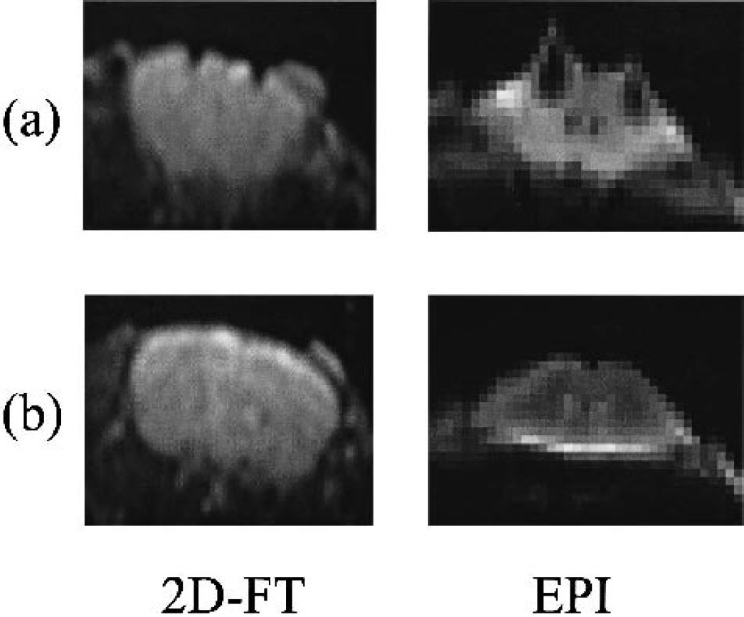
Comparison of echo planar imaging (EPI) and spin echo images at (A) the level of the electrode position and (B) the translated chosen position of the imaging slice in our study. The 2D-FT images are scout images and have low contrast and signal-to-noise ratio because of the nonoptimal parameters necessary for rapid image acquisition.

FIG. 2.

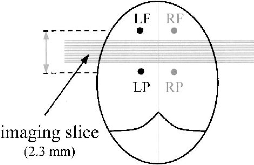
Geometrical layout of the hydrogen electrodes showing the position of the imaging slice. LP, RP, left and right parietal, respectively; LF, RF, left and right frontal, respectively.

To obtain a flow measurement comparable to that obtained from the interstitial MRI slice, mean flow readings in each cerebral hemisphere were determined for both techniques in the following manner. For the HC method, the frontal and parietal electrode readings in each hemisphere were averaged. For the FAIR measurement, regions of interest were drawn on the perfusion maps that encompassed the dorsal portion of the left and right sides in the vicinity of the electrode position.

Temporal matching

In-line filtering of the HC leads allowed simultaneous FAIR and HC measurements. Temporal matching was, therefore, achieved by comparing the simultaneous readings. In one animal, concurrent measurements could not be obtained as a result of interactions between the measurement systems. In this case, the clearance readings were obtained immediately before and after the MRI acquisition, and these readings were averaged.

Experimental protocol

To aid the comparison of the techniques, a series of measurements were obtained over a wide range of relevant flows. After the electrode had been implanted, a time for stabilization was allowed. This is necessary to eliminate the influence of the diffusion barrier, that is, the zone of devitalized and edematous cells that forms around the electrode tip (Aukland, 1965). An initial HC reading was then taken before placing the animal in the magnet. Several paired FAIR and HC measurements of flow were then obtained while the CBF recovered from initially depressed levels. In some preliminary studies, additional FAIR measurements were also performed between the paired measurements, to increase the time resolution of FAIR experiment and improve the definition of the CBF recovery time course. The paired measurements were obtained at approximately 20 to 30 minute intervals. Inversion recovery parameters (T₁, M₀, α₀) were also acquired. Graded occlusion was then initiated in some animals (bilateral n = 3; unilateral n = 2) by tightening the piston device, and the acquisition of simultaneous measurements was continued.

RESULTS

The injurious effect of the clearance electrode insertion was clearly manifested by the initial depression and subsequent recovery of the flows in comparison with published control CBF values in the gerbil. The initial HC reading, obtained at approximately 30 minutes after insertion, was 34 ± 6 mL · 100 g⁻¹ · min⁻¹. Figure 3 shows a time course from an animal that did not undergo occlusion. The flow readings in both hemispheres are displayed from the time of electrode insertion. The initial, depressed HC flow recovered during the following 3 h to a level of approximately 90 to 100 mL · 100 g⁻¹ · min⁻¹ . It can also be seen from Fig. 3 that the HC and FAIR flow time trends are similar.

FIG. 3.

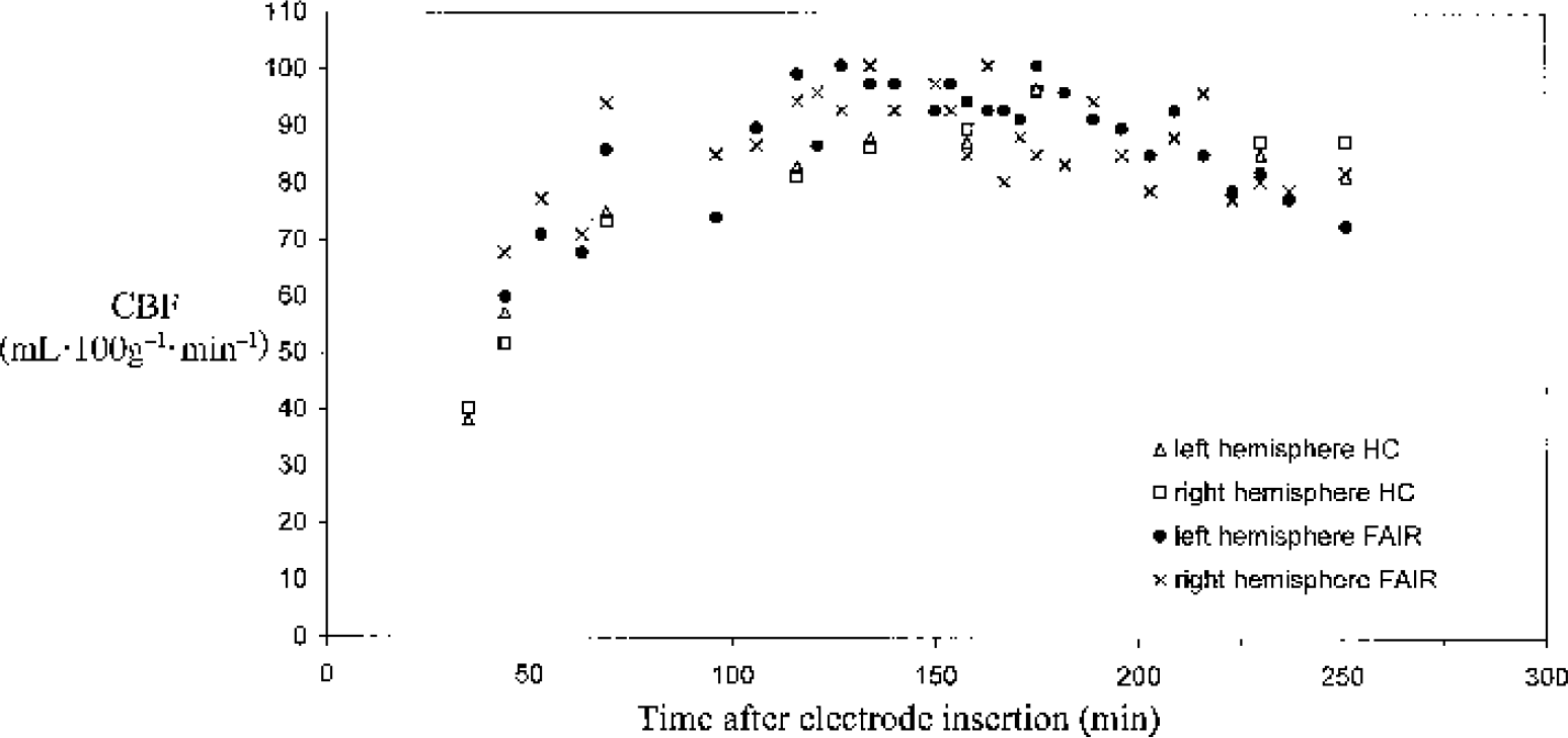
Time course plot of the flow values measured by both techniques in both left and right hemispheres from the time of electrode insertion. In this experiment, additional flow-sensitive alternating inversion recovery (FAIR) measurements were performed between the paired measurements to improve the definition of the cerebral blood flow (CBF) time course. The decreasing flows toward the end of the plot reflect the worsening state of the particular animal. HC, hydrogen clearance.

Mixed model regression

Mixed model regression based on Eq. 1 (equal variances model) yielded the following parameter estimates and, in parentheses, 95% confidence intervals:

$\begin{array}{ll}k=MR:\hfill & {\beta }_{\mathrm{k}0}+0.73(-1.8,+3.2)\text{ml}/100\mathrm{g}/min\hfill \\ \hfill & {\beta }_{\mathrm{k}1}=-0.026(-0.089,+0.037)\hfill \\ k=HC:\hfill & {\beta }_{\mathrm{k}0}=-0.73(-3.2,+1.8)\text{ml}/100\mathrm{g}/min\hfill \\ \hfill & {\beta }_{\mathrm{k}1}-0.026(-0.037,+0.089)\hfill \\ \hfill & {\sigma }_{\mathrm{e}}^2=54.7(42.2,73.7){(\text{ml}/100\mathrm{g}/min)}^2\hfill \end{array}$

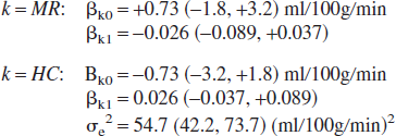
where β_k0 and β_k1 are the location and scale shifts, respectively. It should be noted that a design matrix coding was used in which the location and scale shifts are split equally between the two methods to emphasize that neither is treated as a gold standard method. It should also be noted that in the absence of a scale shift, a value of zero is obtained for β_k1 because it forms part of an additive term (Eq. 1). The location and scale shift parameter confidence intervals span zero, indicating an absence of evidence for a systematic relative bias. Given the size of the confidence intervals, we are not able, however, to rule out a nonnegligible bias relative to the requirements of all conceivable applications. If it is assumed that the systematic disagreement between the HC and MR observations is due entirely to bias in the MR observations and that the HC observations are free of bias, the regression model provides an estimate of 20.4 (17.0, 23.9) mL · 100 g⁻¹ · min⁻¹ and 96.3 (87.9, 104.7) mL · 100 g⁻¹ · min⁻¹ for the population mean MR flow estimate given a true CBF of 20 and 100 mL · 100 g⁻¹ · min⁻¹, respectively. This yields relative bias estimates of 0.4 (−3.0, 3.9) ml · 100 g⁻¹ · min⁻¹ and −3.7 (−12.1, 4.7) mL·100 g⁻¹ · min⁻¹ at 20 and 100 mL · 100 g⁻¹ · min⁻¹, respectively.

Structural equations modeling

An essential component of the mixed model regression analysis was a model-building phase in which various random coefficient terms were assessed for importance. Although Akaike's Information Criterion indicated the superiority of the random coefficients model given in Eq. 1 relative to a reduced model with no random coefficient terms, the difference was borderline. Accordingly, a second-stage analysis was performed in which the random coefficients were dropped. This allows a standard structural equations modeling evaluation of the relative bias in MR observations for comparison with the mixed-model regression results. The constrained variances version of the structural equations model (Eq. 2) yielded the following coefficients, variances (var) and standard errors (SE):

$\begin{array}{lll}\hspace{1em}\hspace{1em}\hspace{1em}{\beta }_0\hfill & =\hfill & 3.84(\text{SE}=1.08)\text{ml}\cdot 100{\mathrm{g}}^{-1}\cdot {min}^{-1}\hfill \\ \hspace{1em}\hspace{1em}\hspace{1em}{\beta }_1\hfill & =\hfill & 0.94(\text{SE}=0.02)\hfill \\ var(r{\epsilon }_{HC})\hfill & =\hfill & var(r{\epsilon }_{MR})\hfill \\ \hfill & =\hfill & 73.7(\text{SE}\hfill \\ \hfill & =\hfill & 9.6){(\text{ml}\cdot 100{\mathrm{g}}^{-1}\cdot {min}^{-1})}^2\hfill \end{array}$

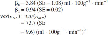
These coefficients provide an estimate of the systematic disagreement between the MR and HC observations on a measurement scale defined by the HC observations. Near identical values for β₀ and β1 were obtained when the equal variances constraint was lifted. The resulting unconstrained variances model, which is just-identified (i.e., with zero degrees of freedom), yielded var(ε_MR) > var(ε_HC), but these variances were estimated with poor precision, and so this inequality must be viewed with caution. Unfortunately, it is not feasible to obtain simultaneous estimates of both the relative bias and variance parameters with good precision. This is because it is not possible to hold blood flow constant while replicate measurements are acquired.

The mixed model regression and structural equations analyses give similar estimates for the magnitude of the location and scale disagreement between the two methods (mixed model regression estimate of the disagreement in scale = 2 × β_k1 = 2 ×(−0.026) = −0.052 (see Eq. 1), compared with the SEM estimate of the scale disagreement = (β₁−1) = (0.94−1) = −0.06 (see Eq. 2); mixed model estimate of the location disagreement = 2 × β_k0 = (2 × 0.73) = 1.46, compared with the SEM location disagreement = β₀ = 3.84). The worst case SEM estimate of the bias in the MR observations (based on an assumption that any systematic discrepancy between the two methods is due entirely to bias in the MR observations, and assuming no bias in the HC observations) yields mean flow rates of 22.6, 50.8, and 97.8 mL · 100 g⁻¹ · min⁻¹ given true flow rates of 20, 50, and 100 mL · 100 g⁻¹ · min⁻¹, respectively (bias = 2.6, 0.8, and −2.2 mL · 100 g⁻¹ · min⁻¹). The unconstrained variances model provides a value of 9.6 mL · 100 g⁻¹ · min⁻¹ for the SD of the MRI random measurement error (but the precision of this estimate is poor), whereas the constrained model gives a SD of 8.6 mL · 100 g⁻¹ · min⁻¹ [var(error) = 73.7, SE = 9.6].

Concordance correlation coefficient analysis

Using the Akaike's Information Criterion results obtained as part of the mixed model regression analysis as justification, the multilevel nature of the study (repeated measurements nested within subjects) was disregarded and a standard concordance correlation coefficient (Lin, 1989) calculation was undertaken (Table 1). The confidence interval obtained for the concordance correlation coefficient indicates a nontrivial departure from perfect concordance, mainly attributable to imprecision, as indicated by ρ. The scale- and location-shift estimates are consistent with a minimal level of bias, hence the observed value for C_b, which is close to unity.

TABLE 1.

	ρc	ρc (lower 95% CI)	ρc (upper 95% CI)	ρ	Cb	v (scale shift)	u′ (absolute location shift) [ml/100 g/min]
Pooled	0.887	0.847	0.916	0.894	0.992	0.982	0.313

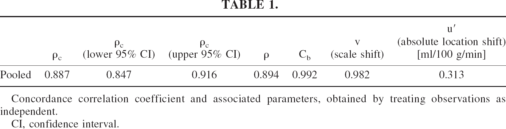
Concordance correlation coefficient and associated parameters, obtained by treating observations as independent.

CI, confidence interval.

A scatter plot of the paired flow readings pooled from all the animals is displayed in Fig. 4. A plot of the difference between the paired MRI and HC observations against their mean is shown in Fig. 5. The overall mean difference in flow (HC-FAIR) is −0.32 ± 14.1 mL · 100 g⁻¹ · min⁻¹ (mean ± SD), and is indicated on the plot together with limits given by twice the SD. Given a normal distribution of observations, approximately 95% of the values should lie between these limits. There is no indication of a relation between the paired-observation differences and the mean value, but there is a suggestion that the variance of the differences is greater at larger mean values.

FIG. 4.

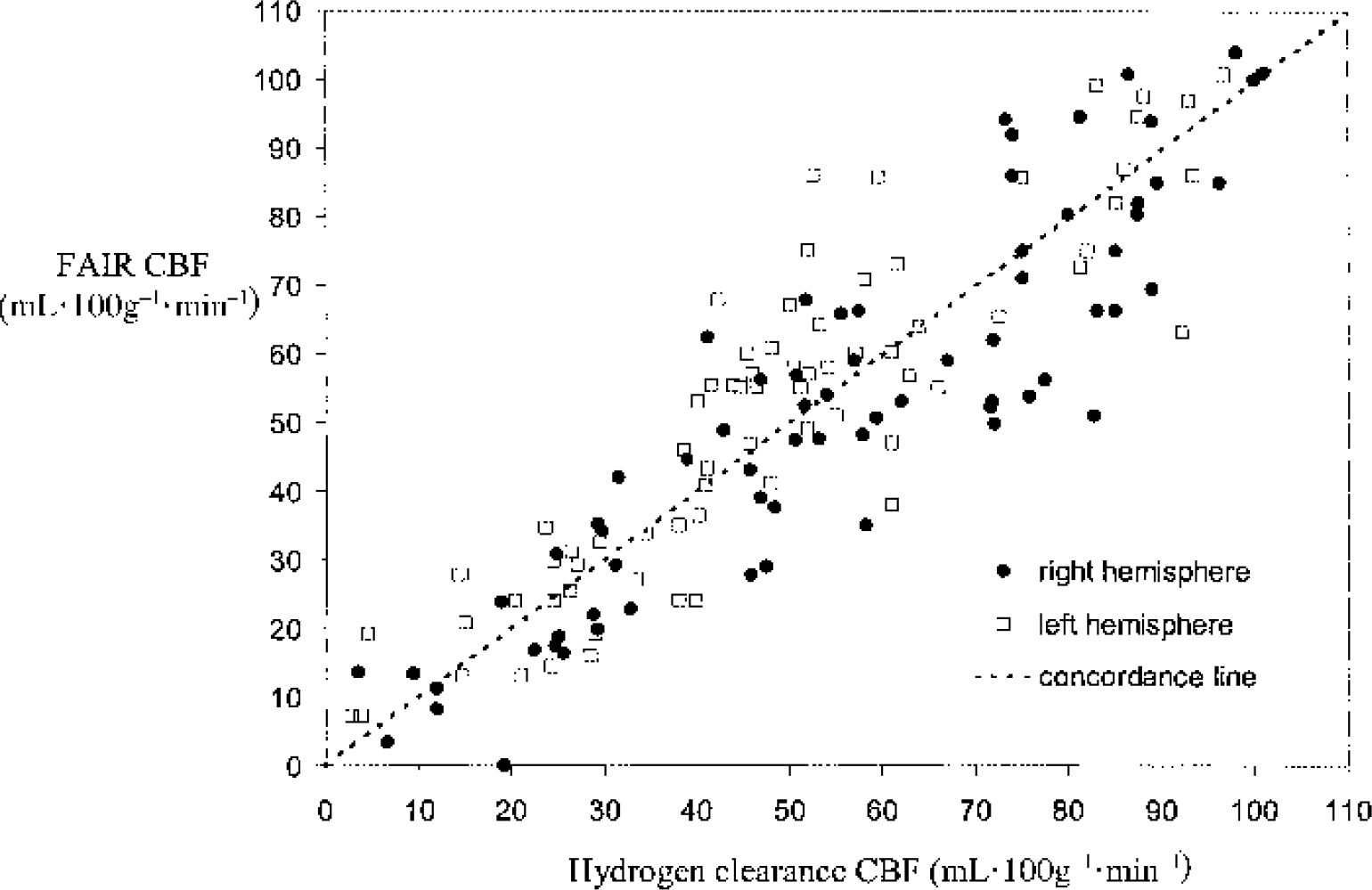
Scatter plot of the paired readings in both hemispheres in the pooled trials (n = 8). FAIR, flow-sensitive alternating inversion recovery; CBF, cerebral blood flow.

FIG. 5.

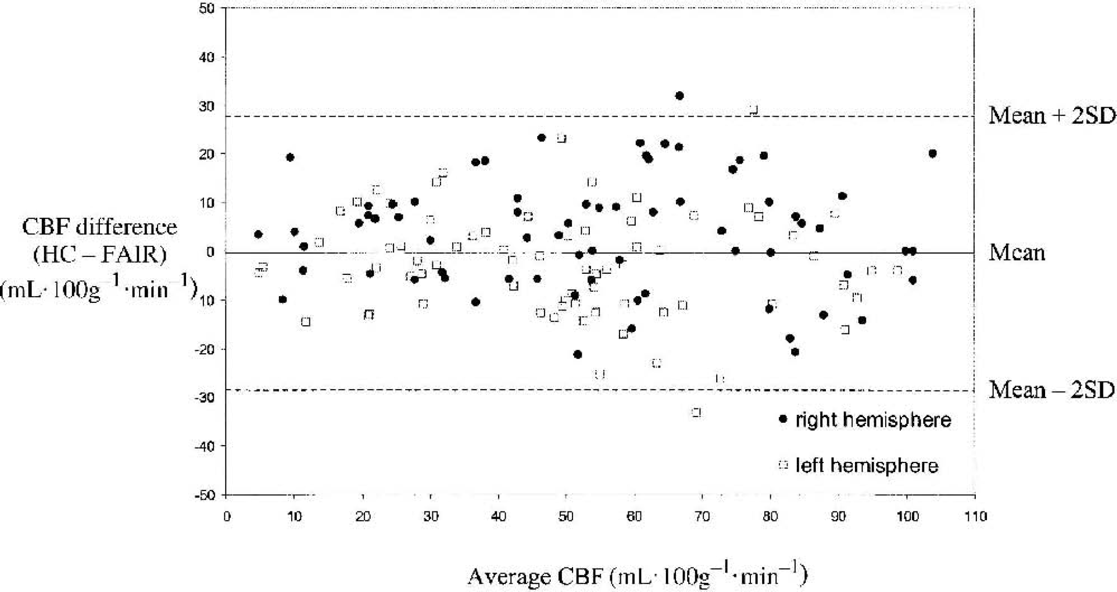
Difference flow plot (hydrogen clearance–magnetic resonance imaging [HC-MRI]) of the paired flow readings from all experiments (n = 8). The differences are plotted against the average flow value given by (HC + MRI)/2. The mean difference is shown together with the (mean + 2 SD, so 2 SD) and (mean − 2 SD, so 2 SD) levels. FAIR, flow-sensitive alternating inversion recovery; CBF, cerebral blood flow.

DISCUSSION

The initial flow measurements obtained after HC electrode insertion compare well with the values typically reported in the gerbil in previous studies using the clearance method in small animals (Busza et al., 1992) but are considerably lower than typical flow values measured by techniques such as autoradiography (Kato et al., 1990). However, a good degree of linear correlation has been reported in the literature between HC and other measurement techniques (LaMorgese et al., 1975; Heiss and Traupe, 1981), although, as discussed previously, this is not a satisfactory means of validation. It has also been noted that the absolute values measured with HC are often considerably lower than expected (Verhaegen et al., 1992). Recognition that this is a real disruption to flow that occurs as a result of electrode insertion, rather than an artefact of the HC technique, has not often been appreciated. A transient flow reduction in the entire cerebral hemisphere has been linked to the induction of waves of spreading depression subsequent to electrode insertion (Tomida et al., 1987; Verhaegen et al., 1992). The placement of platinum electrodes of diameter 250 μm was found to consistently induce spreading depression waves that were detected by the clearance electrodes. The rate of appearance of the spreading depressions is strongly influenced by the electrode size and the insertion depth. On implantation of small electrodes (50-μm diameter) at a depth of 1 mm into the cortex, flows of 155 ± 18 mL · 100 g⁻¹ · min⁻¹ were obtained that were in agreement with values measured with the [³H]-nicotine indicator fractionation technique (Verhaegen et al., 1992). However, the CBF measurements in that study were not carried out in the same animal. Our study has confirmed these findings of initially depressed clearance flows by the simultaneous acquisition of paired MRI-HC measurements. The recovery of flow in our study, as observed using both FAIR and HC (Fig. 3), during the subsequent 3 to 6 hour period, mirrors results obtained by Tomida et al. (1987) and by Verhaegen et al. (1992).

Since the inception of MR methods for perfusion measurement, several authors have attempted to validate these techniques by comparison with non-MRI methods. The non-ASL methods of dynamic susceptibility contrast imaging and deuterium (D₂O) imaging have been compared using single-photon emission computed tomography and microspheres, respectively (Ernst et al., 1999; Simpson and Evelhoch, 1999). The majority of ASL validation studies have focused on the continuous labeling approach, and have used microspheres (Walsh et al., 1994; Hernandez et al., 1998), autoradiography (Allegrini et al., 1998; Hoehn et al., 1999; Ewing et al., 2003), and positron emission tomography (Ye et al., 2000). Pulsed ASL methods have been validated with Xenon-CT (Kimura et al., 2001), microspheres (Zhou et al., 2001), and with autoradiography (Tsekos et al., 1998), although in the latter example comparative flows were obtained from previously reported measurements. All the studies claimed reasonably good agreements between values obtained with the MRI values and the validation techniques, although deviations were sometimes reported. The continuous arterial spin labeling (CASL) validation of Walsh et al. (1994) reported a mean error of −32.4 + 20.2%, with the underestimation of the ASL method most significant at higher flows. The studies described by Hernandez et al. (1998) and Hoehn et al. (1999) all showed a location shift of the MRI method with respect to the perfusion marker. The positron emission tomography comparison noted an underestimation of the CASL method in white matter that was attributed to an underestimation of the transit time (Ye et al., 2000). None of these studies except that of Zhou et al. (2001) used simultaneous, serial measurements. Furthermore, even though reasonably high correlations (ρ or R²) were reported in all these studies, such statistical analysis can lead to misleading conclusions (see Statistical Analysis: Background and Methods).

It should be stressed that a proper validation of any new method requires the direct comparison with an accepted gold standard method. In the case of CBF quantification, it may be difficult to claim that such a method does indeed exist. The various techniques can only provide an indirect measure of the desired quantity itself—the volume of blood irrigating a unit mass of tissue in a unit time and oxygen delivery. If this is the case, a strict validation of a new method is impossible, but comparisons with established standards yield estimates of relative bias, and this is useful information. A second objective is to obtain variance estimates. In this study, HC-FAIR pairs of measurements were made simultaneously, thus reducing the effect of underlying physiologic fluctuations in the blood flow on the observed differences. It is difficult, however, to partition the total variation between the two techniques. To obtain useful estimates of precision, replicate data must be acquired with a frequency that is higher than any real physiologic fluctuation. Although the time scale of these fluctuations is not established, it may be short compared with the temporal resolution of both techniques. Despite these difficulties, the present study provides useful information regarding precision.

To attempt a comparative analysis of the reproducibility characteristics of the FAIR method, a means of perfusion assessment was sought that had characteristics similar to those of the MRI measurement. Hydrogen clearance is a well-established method whose quantitative utility has been investigated in comparative studies with other techniques (LaMorgese et al., 1975; Heiss and Traupe, 1981). Hydrogen as a perfusion tracer possesses the ideal properties of free diffusibility and a low water–gas partition coefficient that ensures rapid removal by the lungs. The interval between successive measurements is only limited by the rate of tissue uptake and clearance and by the need to wait for recovery to a stable current baseline. The HC method is, however, subject to several limitations that may affect its performance in a comparative study. The spatial resolution of the clearance method is a matter of some debate. Although some authors have suggested a spatial resolution as high as 0.5 to 1.0 mm³ (Meyer et al., 1971), it is generally believed that the volume of surrounding tissue to which the electrode is sensitive is approximately 5 mm³.

The arterial spin labeling techniques for MRI perfusion measurements are subject to several concerns than can affect the accuracy of the technique (Pell et al., 1999; Calamante et al., 1999; Barbier, 2001). These include transit time effects, the significance of intravascular contamination, and the consequences of incomplete extraction of blood water into the tissue compartment (Silva et al., 1997). The transit time is the delay between the application of the tag and the arrival of the blood in the imaging slice. During this time, the experiment is not perfusion sensitive. For the normal range of flows in the gerbil, the transit time effect is expected to be negligible. In contrast, under the pathologically low flow conditions induced in our study, the influence of transit times will be exaggerated, and this might be expected to be reflected in the observed relative bias, assuming an absence of parallel bias in the HC measurement. However, the scale- and location-shift estimates obtained from all the analytical approaches used in this study were small. In particular, the mean relative bias estimate at low flow is not consistent with a marked, systematic underestimation.

The original tissue model for ASL quantification that has been used in the analysis of the technique described in this report assumes that water is a freely diffusible tracer (Kety, 1951). A single compartment within the voxel is thereby implied with instantaneous exchange between the water in the blood and the extravascular space. However, this has been shown to be an unrealistic assumption. The equilibration of the water within the blood and tissue compartments is diffusion limited and the extraction fraction is less than 100% (Silva et al., 1997). More sophisticated models have been developed that consider the exchange of water between the capillary and tissue spaces (Zhou et al., 2001; St Lawrence et al., 2001; Parkes and Tofts, 2002). The signal difference is described by significantly expanded exponential terms that include parameters such as the permeability-surface area product of the capillaries. Deviations from the true flow have been reported for the higher range of flows in an animal (due to outflow of unexchanged venous blood) (Zhou et al., 2001) and for human flows (due to the T1 difference between the blood and tissue) (Parkes and Tofts, 2002). However, these are often competing effects, and the mean shift parameter estimates obtained in this study are consistent with the absence of a marked level of inaccuracy, although the associated confidence intervals do not rule out a non-negligible relative bias. Also, the MR-HC scatter and difference plots (Figs. 4 and 5) appear consistent with the absence of a marked level of relative bias.

Three analytical methods were adopted to quantify the discrepancy between the MR and HC measures. A first-stage analysis was performed using mixed-model regression in recognition of the possibility that the level of bias might vary between experiments. The analysis provides estimates of the mean (population) relative bias expressed in terms of the location and scale shift parameters, together with their confidence intervals. Both confidence intervals span zero, consistent with the absence of a systematic relative bias [(−3.0, 3.9) at 20 mL · 100 g⁻¹ · min⁻¹ and (−12.1, 4.7) at 100 mL · 100 g⁻¹ · min⁻¹]. A secondary outcome of the mixed-model regression analysis was the demonstration that the between-subject variability in relative bias (as represented by the random coefficients) is of borderline importance. Whereas these terms were retained in the first stage of the analysis, their removal permits a standard structural equations modeling assessment of the discrepancy between the MR and HC measurements. The two approaches yield consistent results. Structural equations modeling was also used to obtain estimates of measurement precision under various models for the systematic disagreement between the MR and HC measures; a maximum SD of 9.6 mL · 100 g⁻¹ · min⁻¹ was obtained for the MR random measurement error. An ideal study of measurement precision demands the acquisition of replicate measurements at each level of flow. Physiologically driven fluctuations in CBF render this impossible, however, and the large standard error associated with the SD estimate is an inevitable consequence of the resulting lack of replication. Having shown by mixed model regression that the multilevel nature of the present study can be ignored, a simple concordance correlation calculation is justified. As outlined in the Statistical Methods section, the concordance correlation coefficient provides a combined sensitivity to precision (ρ) and accuracy (C_b). In the present context, however, ρ and C_b are of considerable interest in their own right and provide confirmation of the mixed model regression. SEM results indicating that, although a considerable degree of imprecision exists among the observations, the relative bias in the FAIR perfusion data is small.

The analytical methods outlined in this article (mixed model regression, SEM, and concordance correlation coefficient calculation) provide a quantitative assessment of the discrepancy between the HC and MR flow measurements. Whether the level of bias reported in this article is of practical importance clearly depends on the intended application. For example, a mean relative bias of −3.7 (confidence interval −12.1, 4.7) mL · 100 g⁻¹ · min⁻¹ at 100 mL · 100 g⁻¹ · min⁻¹ was obtained by mixed model regression, decreasing in magnitude as CBF decreases towards 28 mL · 100 g⁻¹ · min⁻¹, below which the relative bias becomes positive. This level of bias should be sufficiently small for many practical applications. Similarly, the random measurement error may well be satisfactory for many practical applications, although this is obviously context dependent and a SD on the order of 10 mL · 100 g⁻¹ · min⁻¹ is probably inadequate for any study concerned with precise threshold phenomena. The precision can always be improved through increased image averaging, since the CBF map is based on image subtraction and any improvement in image signal-to-noise gives a proportionate increase in CBF precision, but this may conflict with the time resolution required for certain experiments. It is important to note that the shift-parameter and variance estimates obtained in this study are specific to our experimental conditions. Magnetic field strength, image resolution, hardware performance, and animal/subject size, in addition to signal averaging, are among the important factors that affect the precision and accuracy of the method.

CONCLUSIONS

To summarize, this study compares CBF measurements obtained using FAIR and HC. The mean shift-parameter estimates suggest a level of relative bias in the FAIR measurements that should be sufficiently small in magnitude for many conceivable applications, although the confidence intervals do not rule out a non-negligible bias. The magnitude of the random measurement error may be a limitation in some studies, but the level of precision can be improved by increased averaging, if required.