Absolute Cerebral Blood Volume and Blood Flow Measurements Based on Synchrotron Radiation Quantitative Computed Tomography

Abstract

Synchrotron radiation computed tomography opens new fields by using monochromatic x-ray beams. This technique allows one to measure in vivo absolute contrast-agent concentrations with high accuracy and precision, and absolute cerebral blood volume or flow can be derived from these measurements using tracer kinetic methods. The authors injected an intravenous bolus of an iodinated contrast agent in healthy rats, and acquired computed tomography images to follow the temporal evolution of the contrast material in the blood circulation. The first image acquired before iodine infusion was subtracted from the others to obtain computed tomography slices expressed in absolute iodine concentrations. Cerebral blood volume and cerebral blood flow maps were obtained after correction for partial volume effects. Mean cerebral blood volume and flow values (n = 7) were 2.1 ± 0.38 mL/100 g and 129 ± 18 mL · 100 g^–1 · min^–1 in the parietal cortex; and 1.92 ± 0.32 mL/100 g and 125 ± 17 mL · 100 g^–1 · min^–1 in the caudate putamen, respectively. Synchrotron radiation computed tomography has the potential to assess these two brain-perfusion parameters.

The perfusion parameters cerebral blood volume (CBV) and cerebral blood flow (CBF) are highly related to cerebral hemodynamic changes, such as those observed in brain tumors, stroke, or ischemia. For instance, CBV and CBF assessments are key in the understanding of the tumor growth process, where angiogenesis plays a critical role (Folkman, 1995; Reijneveld et al., 2000). The structure and function of the tumor vessels lead to a chaotic architecture, an irregular blood flow (Carmeliet and Jain, 2000), and an increase in brain perfusion, blood flow, blood volume, and capillary permeability (Miles, 1999). Moreover, brain vasculature functional maps provide a powerful tool for assessing glioma grade and focal activity. It has been shown that high CBV values are associated with mitotic activity and dense vasculature (Aronen et al., 1994).

Most of the medical imaging methods have been used to quantify these parameters in vivo and to build functional maps of the brain. Positron emission tomography (PET) is the admitted reference for in vivo CBV and CBF measurements because it is quantitative and relatively noninvasive (Huang et al., 1983; Phelps et al., 1982; Ter Pogossian and Herscovitch, 1985), whereas magnetic resonance imaging (MRI) is a promising alternative for in vivo brain perfusion studies. A wide range of such methods has recently been reviewed by Barbier et al. (2001). The bolus-tracking techniques are based on the use of dynamic susceptibility (Ostergaard et al., 1996; Rempp et al., 1994) or dynamic relaxivity (Dean et al., 1992; Hacklander et al., 1996) contrast. The CBV can also be measured by steady-state methods, using either susceptibility or relaxivity contrast (Barbier et al., 2001). Computed tomography (CT) scanners could be a good alternative imaging method because of their ready availability and excellent spatial resolution. There are two major ways to assess brain perfusion using a CT scanner. The first method is stable xenon computed tomography, where CBF is measured after the inhalation of xenon, which is used as a freely diffusible tracer (Gur et al., 1989; Johnson et al., 1991; Lee et al., 1990; Nambu et al., 1995). Xenon CT is performed under steady-state conditions and CBF is obtained by using Kety's application of the Fick principle of indicator dilution, which states that tissue uptake of an indicator is supplied by the arterial blood minus the amount carried away by the venous blood. The Kety-Schmidt equations are modified for the xenon CT technique to measure the blood flow with the relation between the time-dependent brain and arterial xenon concentrations (Gur et al., 1989; Johnson et al., 1991; Lassen and Perl, 1979). The second method is dynamic CT, where iodinated contrast agent is infused as an intravascular tracer. The theoretical aspects of this technique have been widely studied (Axel, 1980; Cenic et al., 1999; Gobbel et al., 1991a; Hamberg et al., 1996a, b ; Jaschke et al., 1987) and have been validated with animal and clinical experiments (Cenic et al., 2000; Gobbel et al., 1991b; Nabavi et al., 1999a, b ). For dynamic CT, most of the brain perfusion measurements are based on Axel's work (Axel, 1980) using the time-course changes in the iodine concentration after the infusion of a bolus of iodinated contrast agent. In this model, the CBV, CBF, and mean transit time calculations are theoretically derived from the nondiffusible tracer kinetic theories (Lassen and Perl, 1979; Meier and Zierler, 1954; Zierler, 1962) applied to dynamic CT bolus tracking methods, since the contrast agent remains intravascular.

For quantification purposes, both methods assume a linear relation between the contrast-agent concentration and the CT values (Axel, 1980; Jaschke et al., 1987; Lee et al., 1990). The limits of conventional scanners in quantifying attenuation coefficients, and thus contrast-agent concentrations in tissues, are mainly due to characteristics of the x-ray tube itself (i.e., source size, intensity variations, limited flux, and wide energy spectrum). There is a systematic drift in CT values (Bews et al., 1990; Kearfott et al., 1984) that needs to be corrected before quantitative interpretation (Kearfott et al., 1984; Thaler et al., 1979). Scattering of the x-ray beam is another problem contributing to the imprecision of the CT values. The detection of scattered radiation in conventional CT causes artefacts by inducing nonlinear errors in the measurement of the attenuation coefficients, and hence also imposes the use of correction techniques (Joseph and Spital, 1982; Vetter and Holden, 1988). The broad energy spectrum produced by conventional x-ray generators leads to beam hardening. Since the matter preferentially absorbs low-energy photons, the beam spectrum is modified, which introduces nonlinearities into Beer's law (Brooks and Di Chiro, 1976; Young et al., 1983). This phenomenon is important in the presence of high-absorption materials such as bone or contrast agent (Joseph and Ruth, 1997; Lee et al., 1990; Ruth and Joseph, 1995). Corrections are needed to assume the linear relation between contrast-agent concentration and CT enhancement (Guthaner et al., 1983; Joseph and Ruth, 1997).

A scanner based on a synchrotron source, which provides monochromatic and parallel x-ray beams, leads to performances close to the theoretical limits and thereby opens new directions for medical imaging (Charvet et al., 1998; Dilmanian et al., 1991; Dilmanian, 1992; Elleaume et al., 1999; Le Bas et al., 1995; Lewis, 1997; Thomlinson et al., 2000). A synchrotron x-ray beam produced by a wiggler is stable and naturally collimated in the forward direction, producing a horizontal fan beam. At 150 m from the source, the beam used at the medical beamline at the European Synchrotron Radiation Facility (ESRF) is about 1 mm high and 150 mm wide (Elleaume et al., 1999). It has a wide spectrum and a very high flux, several orders of magnitude higher than those of a conventional x-ray tube (Dilmanian et al., 1991; Lewis, 1997; Thomlinson et al., 2000). These properties make the synchrotron the most suitable source for producing monochromatic x-ray beams with a sufficient flux for medical CT imaging (Dilmanian, 1992; Thomlinson et al., 2000). An advantage of a monochromatic x-ray beam in CT is the absence of beam-hardening effects. Synchrotron beams are nearly parallel, which allows the positioning of the detector far behind the imaged sample, thereby eliminating the detection of the scattered beam (Dilmanian, 1992; Thomlinson et al., 2000). Without the detection of scattered photons and without beam-hardening effects, synchrotron radiation computed tomography (SRCT) allows one to derive accurate quantitative attenuation coefficients maps from the CT data.

Absolute contrast-agent concentration can be derived using energy subtraction (Dilmanian et al., 1991, 1997; Dilmanian, 1992; Elleaume et al., 2000) or temporal subtraction techniques (Dilmanian et al., 1997; Elleaume et al., 2002). Le Duc et al. (2000) produced the first feasibility report of in vivo rat brain CT images using synchrotron radiation. The accuracy and precision of monochromatic CT performance have been assessed with phantom studies (Dilmanian et al., 1997; Elleaume et al., 2002). The measurement accuracy depends mainly on the x-ray dose or photon flux, the beam energy, the contrast-agent concentration, and the object dimension (Dilmanian et al., 1997). The aim of the present study was to obtain absolute values of CBV and CBF using SRCT in vivo and to show that SRCT is a powerful tool for quantitative brain-perfusion assessment.

MATERIAL AND METHODS

X-ray beam and imaging device

All experiments were performed at the medical research beamline at the ESRF. An extensive description of the medical beamline instrumentation is available elsewhere (Elleaume et al., 1999; Thomlinson et al., 2000). The imaging facility is divided into two parts: a monochromator hutch and an experimental hutch just beyond. The experimental hutch contains a positioning and rotating system 150 m from the source and the germanium detector, 5 m beyond the positioning system. The intensity of the beam delivered by the insertion device is six orders of magnitude higher than that of a conventional x-ray tube over a wide energy range (Charvet et al., 1998; Elleaume et al., 1999). The monochromator is a fixed-exit device, based on two bent Si (1 1 1) crystals in the Laue geometry, providing high-intensity monochromatic x-ray beams tunable in the 18- to 90-keV range. The energy in this experiment was set at 33.5 keV (80-eV energy bandwidth), just above the iodine K-edge. The dimensions of the fan-shaped beam are 150 mm wide and 1 mm high at maximum. The high-purity germanium detector comprises two 432-pixel, 150-mm-wide detection rows with a pitch of 0.35 mm. The detector is read in current integration mode by a high-dynamic-range electronic system (16 bits).

Animal model

All experiments were carried out on male Wistar Wag rats (n = 7), and all operative and animal care procedures conformed with the guidelines of the French Government (decree 87–848 of October the 19th 1987, license 7593 and A38071). Each rat was anesthetized with isoflurane inhalation followed by an intraperitoneal infusion of chloral hydrate 4% (1 mL/100 g body weight), and maintained under anesthesia for several hours by intraperitoneal infusion of half doses of chloral hydrate (0.5 mL/100 g body weight) for 2 h. In the perfusion studies, the left jugular vein was catheterized for contrast-agent infusion. The tail artery was catheterized to record mean arterial blood pressure (Powerlab; AD Instruments, Chalgrove, Oxfordshire, U.K.) and to obtain blood gases measurements (ABL 70; Radiometer, Copenhagen, Denmark). Body temperature was maintained using a thermostatic blanket and monitored by an intrarectal probe (Harvard Apparatus, Holliston, MA, U.S.A.).

After the surgical procedures, each rat was held in a vertical stereotactic frame screwed on a rotation stage and aligned along the axis of rotation, to perform axial SRCT of the rat head. Rats were gradually moved to the vertical position by using a 10-minute motorized procedure. For each rat, the images were acquired 9 mm above the interaural line, an area foreseen as a cell implantation site for further experiments on rats bearing tumor. For the partial volume effect studies, SRCT slices were also acquired at the neck level to image the common carotid arteries and jugular veins.

Synchrotron radiation computed tomography protocol

For each acquisition, each rat underwent 17 rotations in 34 seconds (180°/s). The skin entrance x-ray dose delivered during one turn was 5 cGy. Three seconds after the start of the acquisition, a remote-controlled injector (Mark 5; Medrad, Pittsburgh, PA, U.S.A.) infused a bolus of iodine (Hexabrix; Guerbet, Roissy, France, C = 350 mg/mL, 0.1 mL/100 g body weight) into the jugular vein at a rate of 1.5 mL/s. The temporal evolution of the contrast-agent concentration per voxel is the basic datum necessary to retrieve brain perfusion maps. Because a monochromatic x-ray beam was used, the CT images were directly expressed in absolute values of the linear attenuation coefficients at the corresponding energy (μ_{I, 33.5} in cm^–1). The absolute contrast-agent concentration maps were then obtained by subtracting a reference image (acquired before contrast-agent injection) from all the others and dividing the resulting images by the iodine mass attenuation coefficient (μ/p), which was equal to 34.94 cm²/g at 33.5 keV (Dilmanian et al., 1997; Elleaume et al., 2002).

The reconstruction is performed using the SNARK89 filtered back-projection algorithm (Medical Image Processing Group, University of Pennsylvania, Philadelphia, PA, U.S.A.) (Herman et al., 1989) on 180° (1 s/image) by using a parallel-beam approximation. Interleaved images were calculated every 45°, which corresponds to one image every 0.25 seconds. A series of 125 SRCT images was obtained that directly reflected the absolute contrast-agent concentrations in the animal brain during the time course of the bolus (Fig. 1). The spatial resolution of the CT slice was 0.35 × 0.35 mm, and the slice thickness was 0.5 mm.

FIG. 1.

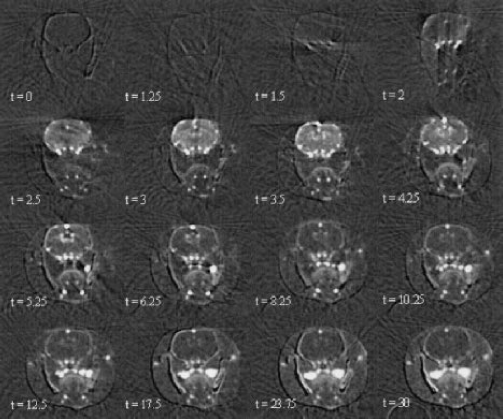
Head axial time-course of iodine concentration maps (mg · mL^–1) on a healthy rat obtained by synchrotron radiation computed tomography, after a bolus infusion (only 16 of 125 images are displayed). Time (t) is expressed in seconds; the infusion starts at t = 0. Iodine enters the brain vasculature via the arterial inputs, passes through the brain microvasculature and is washed out by the intracerebral and extracerebral venous outputs.

The signal-to-noise ratio (SNR) was defined as (Young et al., 1995):

$\text{SNR}=\frac{{\mathrm{M}}_{\mathrm{S}}}{{\mathrm{S}}_{\mathrm{N}}},$

(1)

where S_N is the noise standard deviation, calculated in a wide region of interest (ROI) outside the rat head (75,000 pixels), and M_S is the mean signal of a homogeneous ROI in the rat brain. Slice thickness was chosen based on the compromise between a high SNR and a good spatial resolution, and was set at 0.5 mm with vertically defining slits. Increasing the amount of contrast agent infused improves the SNR, but is antithetic to the needs for a short bolus. The bolus has to provide a small amount of contrast agent per body weight in a short-duration pulse, to minimize the induced physiologic effects. The volume of the infused iodinated contrast agent was 0.1 mL/100 g body weight at 1.5 mL/s, similar to the values commonly used in the literature (Cenic et al., 1999; Hamberg et al., 1996a). In this case, in the caudate putamen (70-pixel ROI) the SNR is equal to 3 with S_N corresponding to a 55-μg · mL^–1 iodine concentration.

Simulations: Accuracy and precision of the concentration measurements

Simulations have been carried out to assess the accuracy and the precision of the iodine concentration measurements. These simulations are computed with the SNARK89 software (Elleaume et al., 2002), and the geometry used simulates a CT slice of a rat head. An ellipse filled with muscle equivalent linear attenuation represents the head (dimensions: 3 × 2.5 cm). The skull is a bone elliptical ring (15 × 10 mm and 0.6 mm thick); two other bone rings stand for the jaws. The brain is considered to be a solution of iodine and water at a concentration equal to 0.125 mg · mL^–1 (i.e., mean brain tissue iodine concentration observed during the bolus passage). A circle 3 mm in diameter, located in the middle of the right hemisphere, was filled with various concentrations of iodine ranging from 0.1 to 25 mg · mL^–1. An iodine-free reference brain slice was also simulated and used as the mask image for the temporal subtractions. CT simulations were performed using entry parameters matching the experimental conditions (flux, geometry, and a skin entrance dose of 5 cGy per slice). A random photonic noise was introduced in the simulated beam. The iodine concentration was calculated in a 2-pixel-radius circular ROI centered in the middle of the iodinated area with IDL data processing software (Research System Inc., Boulder, Colorado, U.S.A.), which allows one to draw circular n-pixel radius ROIs on the slice (where n is the integer representing the radius). The ROI was then defined as the shape made with pixels arranged in a square pattern that best fits the circle. The mean concentration (M_S) and its standard deviation were derived from 10 simulations. The noise S_N in the image was computed in a large ROI outside the simulated rat head, where no signal was present. The accuracy and the precision of the iodine concentration measurements were derived from these simulations.

The accuracy was assessed by the difference between the true value and the measured value. This difference divided by the true value gives the relative error, which was computed by subtracting the true concentration from M_S and dividing the result by the true concentration. A relative error less than 1% was found for the range 0.35 to 1 mg/mL iodine, which corresponds to usual concentrations measured in the brain tissue. A relative error less than 3% was found for the range 2 to 25 mg/mL iodine, which corresponds to usual concentrations measured in the blood vessels. The standard deviation of the averaged iodine concentration measurements, calculated within a 2-pixel-radius ROI, was equal to 10 μg/mL iodine, and was not dependent on the iodine concentration. In the simulations, a noise equal to 40 μg/mL iodine was obtained, comparable to the 55 μg/mL observed in the SRCT measurements.

Recirculation and γ-variate fitting

To apply the indicator dilution theories, it was essential to consider the recirculation phenomenon in the iodine concentration–time curves (Axel, 1980; Meier and Zierler, 1954). Infusion time has to be as short as possible to get a bolus duration in the tissue that is shorter than the recirculation time (Axel, 1980). It is possible to assess the recirculation time (tr_eci_rc.) by adding the time t1 between the iodine entrance in the common carotid artery and its appearance in the jugular vein to the time t₂ needed for the blood to go through the right heart, the pulmonary vasculature, and the left heart to the common carotid artery. The delay t₂ is assumed to be equal to the delay observed between the beginning of a given infusion and the iodine entrance in the common carotid artery. The measurement of the recirculation in four rats yielded t₁ = 2.625 ± 0.32 seconds, t₂ = 0.625 ± 0.14 seconds, and t_recirc = 3.25 ± 0.35 seconds. The infusion duration (0.17 seconds) was 20 times shorter than the recirculation time. The bolus duration in the brain tissue was calculated in a homogeneous ROI (drawn in the right caudate putamen) as the full width half maximum of the ROI iodine time–concentration curve. The mean value (2.1 ± 0.43 seconds) was less than the recirculation time.

γ-Variate functions are used for fitting bolus temporal concentration curves. They match the fast rise of the iodine concentration in the tissue during its entrance, and its monoexponential washout (Thompson et al., 1984). This mathematical model for bolus transit in tissue is widely used for brain perfusion imaging (Gobbel et al., 1991b; Hamberg et al., 1996a; Ostergaard et al., 1996; Rempp et al., 1994). Time–concentration curves of each voxel are fitted with a γ-variate function of the following equation by using the downhill simplex method (Press et al., 1988):

$\begin{array}{lll}{C}_{\mathrm{T}}(t)\hfill & =\hfill & C_{\mathrm{p}}{\left(\frac{e}{\alpha \beta }\right)}^{\alpha }{(t-t_{\mathrm{A}})}^{\alpha }exp\left(-\frac{t-t_{\mathrm{A}}}{\beta }\right)\hfill \\ \hfill & =\hfill & K{(t-t_{\mathrm{A}})}^{\alpha }exp\left(-\frac{t-t_{\mathrm{A}}}{\beta }\right),\hfill \end{array}$

(2)

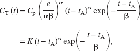
where C_T is the iodine concentration (mg/mL), t is the time (seconds), C_p is the maximal iodine concentration of the voxel (mg/mL), t_A is the iodine arrival time (seconds), α and β are adjustment parameters determining the main curve profile, and K = C_p(e / αβ)^α is an amplitude factor.

Figure 2 shows typical internal carotid artery and right caudate putamen time–concentration curves, obtained in homogeneous ROIs of a 240-g healthy rat brain. The curves were fit by γ-variate functions; the linear Pearson correlation coefficients between the native data and the fitted curves points were 0.99 and 0.97 for the arterial fit and the brain tissue fit, respectively. The first passage of the bolus and a second peak, related to the recirculation phenomenon, appear on the arterial curve.

FIG. 2.

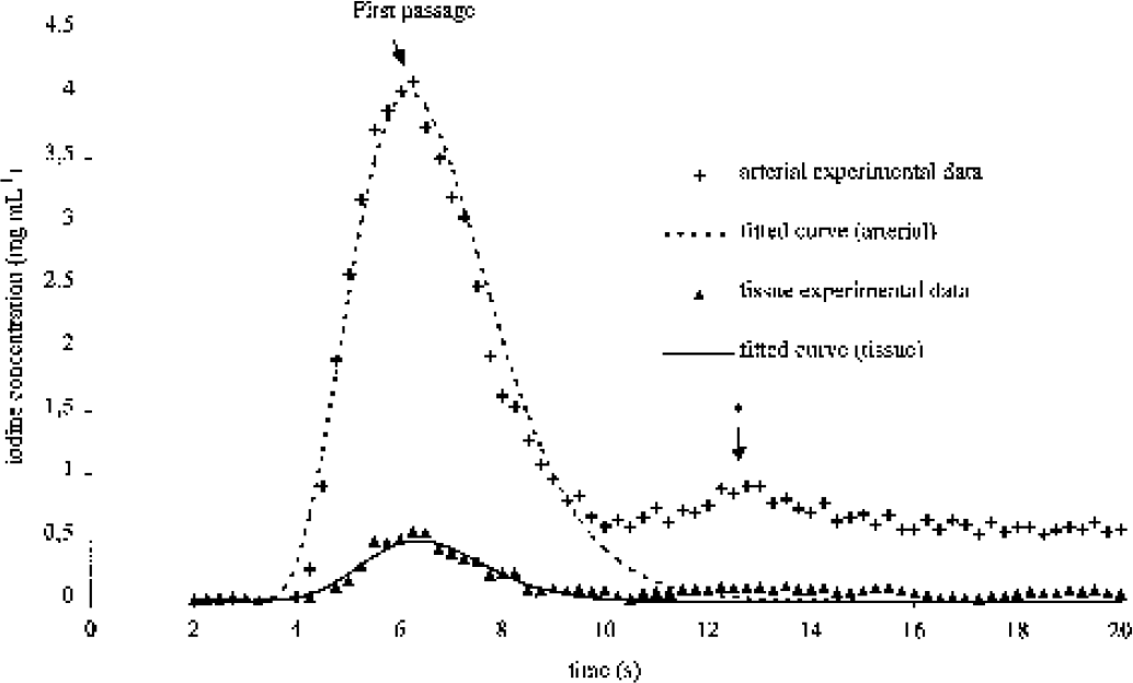
Typical arterial region of interest (ROI) iodine concentration curve and a typical right caudate putamen ROI iodine concentration curve derived from a set of synchrotron radiation computed tomography slices. Both arterial and tissue curves are fitted with a γ-variate function (R² = 0.99 and R² = 0.97, respectively). The peak (*) is related to the recirculation process. The monoexponential fall of the fitted curves limits the recirculation contribution to the bolus curve.

Stationarity and linearity

The stationarity of a system denotes the constancy of all systemic parameters in time. The response to a stimulus (bolus infusion) is fully determined by these systemic parameters. The stationarity was checked between two identical sets of SRCT acquisitions (sequences 1 and 2) performed on the same rat. Two ROIs were controlled: one arterial ROI (in the right internal carotid artery) and one brain-tissue ROI (right caudate putamen). The same amount of iodine (0.15 mL) was infused at the same rate (1.5 mL/s) but delayed in time (after iodine washout). The resulting time–concentration curves were fitted with γ-variate functions. Sequences 1 and 2 provided identical responses, which demonstrated system stationarity and allowed the comparison of SRCT scans acquired in the same conditions at different times. The linearity of the system was confirmed when the response to two combined bolus infusions was the sum of both separate responses to each single-bolus infusion. The comparisons were performed with a simple (sequence 1) and a twofold volume bolus of iodine (sequence 3) (0.15 and 0.3 mL, respectively, at the same rate of 1.5 mL/s). As a result, twofold values for the maximum iodine concentrations and the areas under the time–concentration curves were measured in the sequence 3. Therefore, in our experimental conditions, the rat brain vasculature was considered to be a stationary and linear system, implying that the area under the response curve of any type of bolus was the same if the same amount of contrast agent was infused. Moreover, after an iodinated bolus infusion the system outlets (i.e., all the arteries of the rat body, including the carotid arteries) have identical areas under the concentration curves (Lassen and Perl, 1979). This equality allowed for the comparison of measurements performed in the common carotid artery and in any artery of the skull basis. During these sequences, no significant change in the observed rat physiological parameters was observed.

Measurements

Cerebral blood volume.

The volume fraction, Vf, occupied by the indicator in the studied voxel of tissue is given by the following equation (Axel, 1980; Hamberg et al., 1996a; Ostergaard et al., 1996):

$\text{Vf}=\frac{{\int }_0^{\infty }{C}_{\mathrm{T}}(t)dt}{{\int }_0^{\infty }{C}_{\mathrm{a}}(t)dt},$

(3)

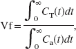
where C_T(t) denotes the evolution of the studied tissue voxel contrast-agent concentrations with time and C_a(t) its arterial input. Owing to the stationarity and linearity of the system, the latter is constant in any arterial input of the CT slice. The recirculation phenomenon has to be avoided when computing the CBV.

Since iodine is a plasmatic tracer, Vf is not the CBV per se, but the cerebral plasmatic volume, and a correction with the hematocrit value is necessary (Meier and Zierler, 1954; Zierler, 1962). By dividing by the mean cerebral tissue mass density, ρ, the following CBV equation is obtained (Rempp et al., 1994; Smith et al., 2000):

$\text{CBV}(\text{mL}/100\hspace{0.17em}\mathrm{g})=\frac{k_H}{\rho }\frac{{\int }_0^{\infty }{C}_{\mathrm{T}}(t)dt}{{\int }_0^{\infty }{C}_{\mathrm{a}}(t)dt},$

(4)

where ρ = 1.08 g/cm^–3, k_H = (1 –HCT_LV)/(1 – HCT_SV) = 0.83 is the factor correcting for the hematocrit value, and HCT_LV and HCT_SV are the hematocrit values in large and small vessels (42% and 30%, respectively) (Bereczki et al., 1993a,b). Each pixel of the SRCT slices provides the tissue concentration–time curve C_T(t) and the selected arterial input provides the input concentration–time curve C_a(t) in (Eq. 4). The CBV is computed for each pixel of the SRCT slice. Mean CBV values were also computed in several ROIs of the brain: the caudate putamen, the frontal cortex, the parietal cortex and the whole brain hemispheres (left and right in each case).

Cerebral blood flow.

It has been shown that the tissue–concentration curve of a given voxel is the convolution of the voxel residue function R(t) (which is the fraction of tracer remaining in the vasculature at time t) with its arterial input, multiplied by the CBF:

${\mathrm{C}}_{\mathrm{T}}(t)=\text{CBF}\cdot {\mathrm{C}}_{\mathrm{a}}(t)\otimes \mathrm{R}(t).$

(5)

Detailed explanations are available elsewhere (Ostergaard et al., 1996; Rempp et al., 1994). Briefly, the tissue residue function R(t) monotonically decreases from 1 to 0. The CBF is the maximum of the curve obtained when the deconvolution of the tissue concentration—time curve with the corresponding arterial input concentration curve is performed. It is crucial that the arterial input chosen is as close as possible to the studied voxel of tissue because this input may undergo dispersion before its arrival in the tissue itself. This dispersion induces errors in the deconvolution process and induces flow underestimation because the shape of the true tissue arterial input is different than that of the selected arterial input (Cenic et al., 1999; Ostergaard et al., 1996). In the present study, the biggest internal artery of the brain was selected as the arterial input, hence allowing for a better correction of the partial volume effects.

The parametric Fourier transform method is used for the deconvolution process. This method is not sensitive to the delays between the curves, as are matrix inversion methods. The CBF values obtained in humans using this method are close to the commonly accepted values measured with PET (Smith et al., 2000). To apply the parametric Fourier transform method, one has to consider continuous periodic functions. This is achievable through the γ-fitting process, providing concentration curves with zero baselines (Smith et al., 2000). A continuous and periodic function is then obtained by repeating periodically the γ curve. Eq. 5 then becomes:

$\begin{array}{l}\text{CBF}\cdot \mathrm{R}(\mathrm{t})[\text{mL}\cdot 100\hspace{0.17em}{\mathrm{g}}^{-1}\cdot {min}^{-1}]=\hfill \\ \hspace{0.17em}\hspace{0.17em}\hspace{0.17em}\hspace{0.17em}\hspace{0.17em}\hspace{0.17em}\hspace{0.17em}\hspace{0.17em}\hspace{0.17em}\hspace{0.17em}\hspace{0.17em}\hspace{0.17em}\hspace{0.17em}\hspace{0.17em}\hspace{0.17em}\hspace{0.17em}\hspace{0.17em}\hspace{0.17em}\hspace{0.17em}\hspace{0.17em}\hspace{0.17em}\hspace{0.17em}\hspace{0.17em}\hspace{0.17em}\hspace{0.17em}\hspace{0.17em}\hspace{0.17em}\hspace{0.17em}\hspace{0.17em}\hspace{0.17em}\hspace{0.17em}\hspace{0.17em}\hspace{0.17em}\hspace{0.17em}\hspace{0.17em}\hspace{0.17em}\hspace{0.17em}\frac{fac}{\rho }{F}_T^{-1}\left(\frac{F_{\mathrm{T}}(C_{\mathrm{T}}(t))}{F_T(C_{\mathrm{a}}(t))}\right),\hfill \end{array}$

(6)

where ρ = 1.08 g · cm^–3 is the brain tissue density, fac = 6,000 is a conversion factor for expressing CBF in mL · 100 g^–1 · min^–1, F_T is the Fourier transform operation, and F_T^–1 is the inverse Fourier transform operation.

This deconvolution process is extremely sensitive to noise; undesirable and meaningless high frequencies in the deconvolved curves lead to oscillations of high intensity as shown in Fig. 3A (Gobbel and Fike, 1994; Ostergaard et al., 1996; Smith et al., 2000). A low-pass filter removes the noise in the residue curve without modifying the underlying values (Gobbel and Fike, 1994). The residue function is then filtered with a low-pass filter of decreasing cutoff frequencies, until a criterion on the residue curve is satisfied. For each cutoff frequency f, the following parameters are computed: R_f(t) the residue function and the error index, Er(f):

$\text{Er}(\mathrm{f})=\frac{\left(\sum _{k=1}^N\mid R_{\mathrm{f},\mathrm{k}}-R_{\mathrm{f},\mathrm{k}-1}\mid \right)-2R_{\mathrm{f},\mathrm{M}}-R_{\mathrm{f},\mathrm{m}1}-R_{\mathrm{f},\mathrm{m}2}}{N(R_{\mathrm{f},\mathrm{M}}-R_{\mathrm{f},\mathrm{m}})},$

(7)

FIG. 3.

(A) Example of a pixel tissue residue curve obtained after deconvolution by the Fourier transform method (black dots, dashed curve). This curve has to be filtered because it contains high-frequency noise. The error index is then calculated with Eq. 7 by filtering this curve with a Butterworth low-pass filter of decreasing cutoff frequencies from 124 to 0 arbitrary units (a.u.). The solid line curve is the residue curve obtained after filtering the dashed line curve by the filter of the optimal frequency cutoff found with the error index curve (B). (B) Error index plotted as a function of the cutoff frequency. In this case the error index decreases with the cutoff frequency and increases again. The optimal error index is the minimal value and gives a cutoff frequency of 41 a.u.

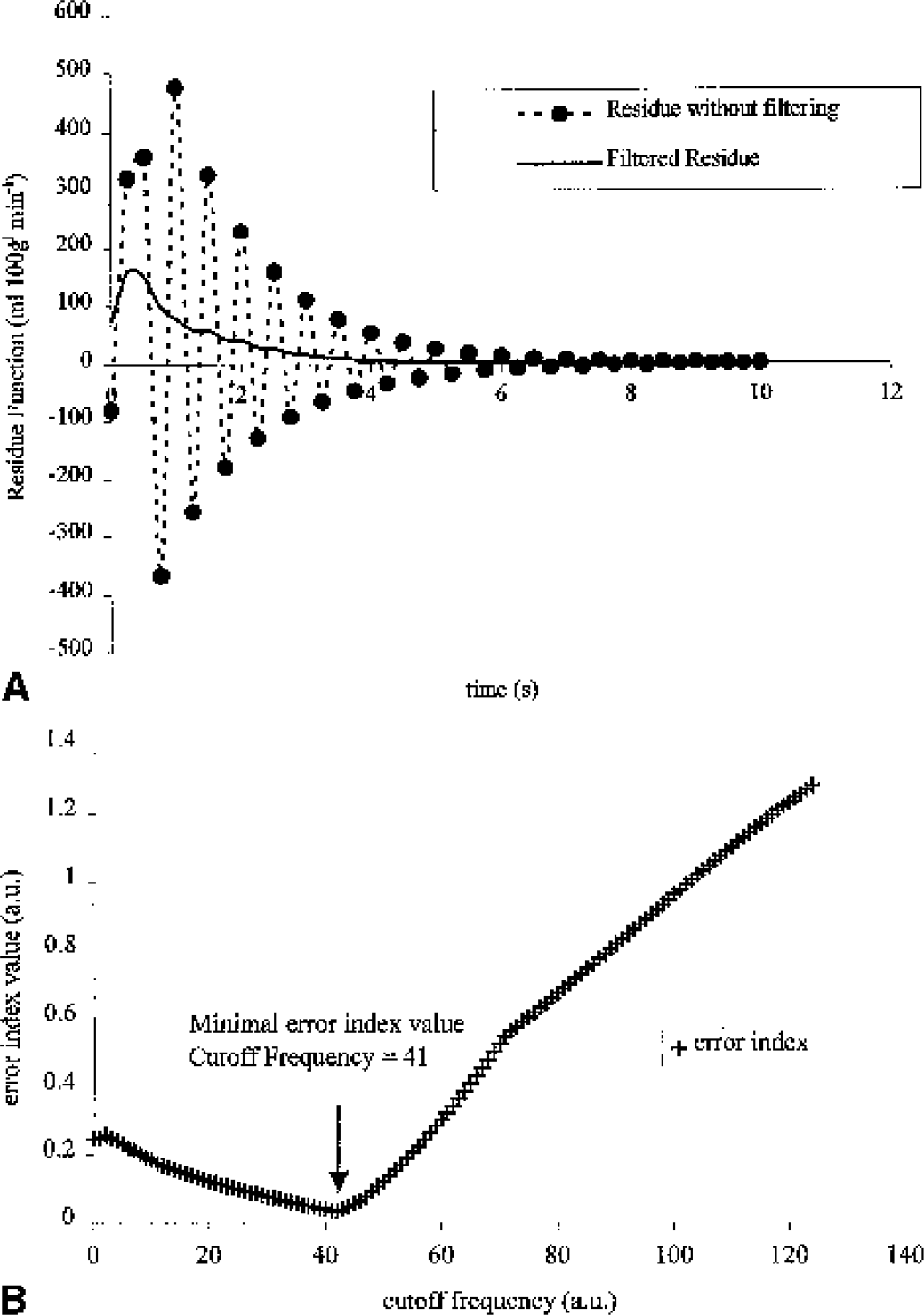
where R_f,k is the k^th element of R_f; N is the number of sampling points of R_f; R_f,M is the maximal value of R_f; R_f,m is the minimal value of R_f; R_f,m1 is the minimal value of R_f for all components R_f,k, k<M, R_f,m2 is the minimal value of R_f for all components R_f,k, k>M.

An Er(f) value close to zero is representative of the unimodality of R(t). The unimodality implies that the concentration of the indicator increases to its maximal value at the time entrance of the indicator in the tissue and then falls monotically to zero as the indicator is cleared from the tissue (Gobbel and Fike, 1994). In this study, Er(f) decreased with f to minimal value, and then increased again (Fig. 3B). This is because once R(t) is unimodal, the numerator of (Eq. 7) is small and stable when f decreases, but R(t) starts to be highly filtered and some information is lost (the value of in the denominator of Eq. 7 decreases as f decreases). The frequency corresponding to this minimal value is the optimal cutoff frequency. In most cases, R(t) is already unimodal after deconvolution; thus, Er(f) increases as f decreases and no filtering is performed. In some cases, Er(f) decreases to 0 with f and then the first cutoff frequency corresponding to Er(f)<0.0625 is chosen (Gobbel and Fike, 1994). Figure 3B shows the selected cutoff frequency used to obtain the filtered residue in Fig. 3A. The CBF is the maximal value of the filtered residue curve.

Partial volume effects

Partial volume averaging is a phenomenon that occurs when small blood vessels are imaged with insufficient spatial resolution: the tracer signal intensity of the vessel is averaged with the signal of the surrounding tissue. Partial volume averaging causes errors leading to an overestimation of the CBV and the CBF (Axel, 1980; Cenic et al., 1999). This problem, inherent to the spatial resolution of the detector, is critical for quantitative measurements when small animals are imaged. The arterial input needs to be corrected for partial volume averaging before the CBV and CBF are computed.

The method used in this article was first described in Cenic et al. (1999). A phantom dedicated to partial volume studies was designed (Fig. 4), and consisted of two lines of cylindrical holes with a diameter range of 0.3 to 1.5 mm and a 5-mm-diameter control hole. SRCT slices of the phantom were acquired with holes filled either with pure water or with iodinated contrast-agent solutions at three concentrations (5, 10, 15 mg/mL) for three series of acquisitions. The SRCT slice image of the phantom filled with water was subtracted from the others to get SRCT slices expressed in absolute contrast-agent concentration. The partial volume scaling factor (PVSF) was then computed by dividing the true concentration measured in the control hole with the concentration measured in the other tubes, for the three iodine concentrations. The concentrations were measured in each tube by using several ROI sizes: the pixel of highest concentration or circles with a radius of 1 to 5 pixels were centered on the tube to assess the effect of the ROI size on the PVSF. The measurements obtained showed that the PVSF value was only related to the diameter of the hole and to the ROI radius. The spatial location of the hole and the contrast-agent concentration did not affect the PVSF value.

FIG. 4.

Synchrotron radiation computed tomography (SRCT) of the partial volume Lucite phantom drilled with two rows of holes (diameters ranging from 0.3 to 1.5 mm, and a 5-mm-diameter control hole), filled with 10 mg · mL^–1 of iodine solution. From the SRCT acquisitions with this phantom, the ratio of the true value over the measured value, the partial volume scaling factor (PVSF) is calculated in various conditions. The PVSF depends only on two parameters: the diameter of the hole and the radius of the circular region of interest used for the measurement.

Figure 5A shows the PVSF as a function of the tube diameter for a 2-pixel-radius measurement ROI. The relation obtained between the PVSF and the tubes diameters was fitted with an exponential function:

$\text{PVSF}=1+36{\text{.8e}}^{-3.49\mathrm{d}}({\mathrm{R}}^2=0.98),$

(8)

FIG. 5.

(A) Partial volume scaling factor (PVSF) versus tube diameter in the case of a two-pixel-radius circular region of interest (ROI). A decreasing exponential fits the curve (R² = 0.98). In this case, the partial volume phenomenon occurs for objects smaller than 1.5 mm. The dashed curve is the result of the PVSF simulations. (B) The PVSF curves fitted with exponential functions of the radius of the circular ROI for three tube diameters.

where d is the tube diameter. Simulations were performed to evaluate the theoretical PVSF compared with the experimental PVSF achievable. The geometry used for these simulations was the same that the one used for the accuracy simulations. The iodine concentration in the right hemisphere circle was set to 10 mg/mL and its diameter varied in the same range as that of the partial volume phantom studies (0.3 to 1.5 mm). The concentration was measured in a 2-pixel-radius ROI centered on the iodinated area and compared with the true concentration to compute the PVSF. After the exponential fit, a simulated PVSF was obtained:

$\text{PVSF}=1+30{\text{.76e}}^{-3\text{.19d}}({\mathrm{R}}^2=0.99).$

(9)

The difference between the simulated and experimental data was negligible for diameters higher than 0.4 mm, showing a good agreement between measured and simulated data.

Figure 5B shows the exponential relation between the measured PVSF and the radius of the tube-measurement ROI in three different tube diameters. The curves are similar for the other diameters.

The correction of the partial volume effects requires the choice of an arterial input, the measurement of its diameter, and the correction with the corresponding PVSF. The in vivo arterial diameter was computed using calibration measurements achieved in the PVSF phantom studies. The concentration profiles (horizontal, vertical, or two dimensional) in the tubes on the reconstructed slice were fit with gaussian curves, and the gaussian standard deviation (GSD) is a linear function of the hole diameter. The following relation was obtained for the horizontal profiles:

$\text{GSD}=0\text{.47d}+0\text{.69}\hspace{0.17em}({\mathrm{R}}^2=0.98)$

(10)

where d is the hole diameter. Similar curves were obtained for the other profiles (vertical or two dimensional). This technique stands for measurements of diameters ranging between 0.4 and 1.4 mm.

The choice of a suitable arterial input is crucial for partial volume corrections because the quality of the in vivo diameter measurement is strongly related to the surrounding structures, the shape and size of the artery. The artery is assumed to be perpendicular to the beam. The artery has to be as isolated as possible from other iodine containing structures, which can enlarge the theoretical profiles, leading to diameter overestimation. Two different input arteries were used for comparison purposes: the common carotid arteries and the most suitable skull basis artery (Fig. 6). The literature gives a diameter close to 0.9 mm for the common carotid artery and 0.7 mm for the internal carotid at its beginning and less for the resulting brain arteries (Scremin, 1995). The kind of profile used (horizontal, vertical, or two dimensional) for the diameter computation depends on the presence of surrounding vessels. The gaussian fits of the chosen profile are performed only on the SRCT slices in which the contrast between the arterial signal and the surrounding signal is high enough leading to a mean diameter and its standard deviation. Fits are rejected when computed diameters are out of the 0.4- to 0.8-mm range for the brain arteries or out of the 0.7- to 1.4-mm range for the common carotid arteries.

FIG. 6.

Synchrotron radiation computed tomography (SRCT) iodine concentration maps of transverse brain slices on two different rats A and B imaged 2.5 seconds after the iodine bolus infusion. The bolus enters the skull basis arteries a1 and a2. a1 is the biggest brain artery with the highest blood flow and is selected as the arterial input in 4 of 5 rats. a2 is a smaller artery selected as the arterial input for one rat because a1 is not isolated in this case. On A are drawn the regions of interest (ROIs) used for the cerebral blood volume and cerebral blood flow computations in this article: the frontal cortex (ROI1), the parietal cortex (ROI2), the caudate putamen (ROI3), the whole hemisphere including blood structures (ROI4), the whole hemisphere without the blood structures (ROI5) and the whole brain (ROI4 left plus ROI4 right). The ROIs content: 15 pixels (pixel size: 0.122 mm²) in ROI1, 40 in ROI2, 65 in ROI3, 1,000 in ROI4, and 700 pixels in ROI5.

The common carotid arteries are isolated and the diameter computation is feasible on many SRCT slices. For the skull basis arteries, the gaussian fit is more difficult to implement. These arteries are smaller and surrounded by veins or tissue, where iodine appears adjacent to the arteries yielding an overestimation of the true diameter. Acceptable diameters were found only on one to five successive SRCT slices, depending on the studied rat. Table 1 shows the mean diameter computation for each considered arterial input, including the number of slices where the gaussian fit provided a reliable result. The standard deviation of the in vivo diameter measurement is accurately assessed with the common carotid arteries, which are isolated and can be considered as references, allowing a high number of different measurements, and thus an averaging on a high number of sampling points (35–103 slices provided reliable diameter measurements, depending on the studied rat). Owing to the small number of sampling points (only 1–5 slices among the 125 available provided reliable diameter measurements, depending on the studied rat) for the skull basis arteries diameter computation, the standard deviation was artificially small and not representative of the true precision.

TABLE 1.

In vivo assessment of the arterial diameters on five healthy rats

Rat no.	1	2	3	4	5
Rat weight (g)	240	240	240	240	330
Common carotid artery
n (number of slices where the gaussian fit provides reliable results)	99	86	103	73	35
Profile	Horizontal	Vertical	Horizontal	Horizontal	2D
Mean diameter ± SD (mm)	1.08 ± 0.15	1.08 ± 0.16	0.97 ± 0.16	1.16 ± 0.17	1.30 ± 0.11
Brain artery
n (number of slices where the gaussian fit provides reliable results)	4	5	3	1	4
Profile	2D	2D	Vertical	Vertical	2D
Mean diameter (mm)	0.66	0.47	0.69	0.65	0.55

For each rat two diameters are computed, in the common carotid artery and in a skull basis artery. The mean diameter is computed on each rat on both common carotid and skull basis arteries. The diameter SD is calculated only for the common carotid because it is meaningless for the small values of n for the brain artery.

Table 2 shows the PVSF computation with the diameters of Table 1 with two arterial measurement ROIs for determining the most suitable ROI size: the highest intensity pixel and a 2-pixel-radius circle centered on this highest-intensity pixel. The areas under the time–concentration curve obtained in the skull basis arteries after correction for the partial volume effects were compared with the corrected areas obtained in the common carotid artery considered as references. These areas have to be equal according to tracer kinetic theory (Lassen and Perl, 1979). The performed comparisons performed in Table 2 show that an input function measurement with a 2-pixel-radius ROI leads to better results than when the simple highest-intensity pixel is used. The mean difference between the two areas after partial volume correction in the case of a 2-pixel-radius ROI is 6.6% compared with 38% in the case of a single-pixel measurement. Larger ROIs provide results of decreasing quality due to the surrounding structures. Thus, CBV and CBF were calculated using a 2-pixel-radius ROI for the arterial input concentration–time curve measurement after the partial volume effect corrections.

TABLE 2.

Reliability and comparison of the partial volume scaling factor computation methods on five imaged rats

	Highest-intensity pixel for arterial input measurement					2-Pixel radius ROI for arterial input measurement
Rat number	1	2	3	4	5	1	2	3	4	5
Common carotid artery
Area under Ca(t) (mg · s · mL–1)	80.96	58.24	60.05	70.87	48.80	28.80	31.73	30.40	39.40	33.19
PVSF (mean ± SD)	1.21 ± 0.16	1.27 ± 0.19	1.35 ± 0.24	1.15 ± 0.15	1.06 ± 0.08	1.97 ± 0.52	2.2 ± 0.57	2.41 ± 0.71	1.77 ± 0.51	1.43 ± 0.3
Corrected area: A1 (mean ± SD [mg · s · mL–1])	97.6 ± 12.6	74 ± 11	80.8 ± 14.38	81.7 ± 10.6	52.1 ± 4.1	56.7 ± 15	69.7 ± 18	73.3 ± 21.8	69.6 ± 20.2	47.5 ± 10.2
Skull basis artery
Area under Ca(t) (mg · s · mL–1)	21.05	16.40	25.65	18.40	9.53	12.10	7.66	16.10	13.03	5.89
PVSF (mean value)	2.25	4.15	2.05	2.29	3.36	4.71	8.21	4.41	4.80	7.60
Corrected area: A2 (mg · s · mL–1)	47.43	68.10	51.60	42.10	32.00	57.03	62.90	68.96	62.54	44.75
Comparison of the corrected areas |(A1 – A2)/A1|	51%	8%	36%	48%	42%	1%	10%	6%	10%	6%

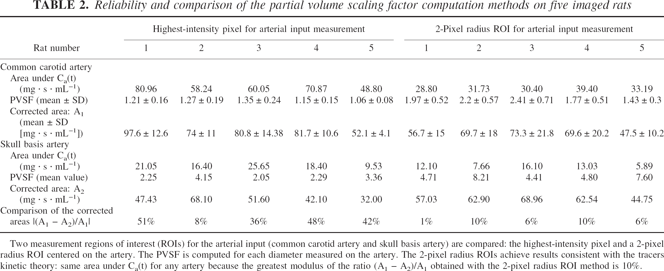
Two measurement regions of interest (ROIs) for the arterial input (common carotid artery and skull basis artery) are compared: the highest-intensity pixel and a 2-pixel radius ROI centered on the artery. The PVSF is computed for each diameter measured on the artery. The 2-pixel radius ROIs achieve results consistent with the tracers kinetic theory: same area under C_a(t) for any artery because the greatest modulus of the ratio (A₁ – A₂)/A₁ obtained with the 2-pixel radius ROI method is 10%.

RESULTS

The functional maps were produced after the computation of CBV or CBF in each pixel of the CT slices. In both cases, the selected arterial input was the brain arterial input corrected for partial volume effects. Figures 7A and 7B show three CBV and CBF maps; a dedicated color palette codes the CBV or CBF values increasing from blue to red. On these maps one can clearly identify the superior sagittal sinus, the skull basis vessels, the cortex superficial vessels, the cortex, the caudate putamen, and the corpus callosum.

FIG. 7.

(A) Transverse cerebral blood volume (CBV) maps of three healthy rat brains. From purple to red the CBV increases from 0 to 100 mL · 100 g^–1. (B) Transverse cerebral blood flow (CBF) maps of the same rat brains used for A. From purple to red the CBF increases from 0 mL · 100 g^–1 · min^–1 up to 1,500 mL · 100 g^–1 · min^–1. Black pixels inside the brain slices indicate voxels where the CBF cannot be determined.

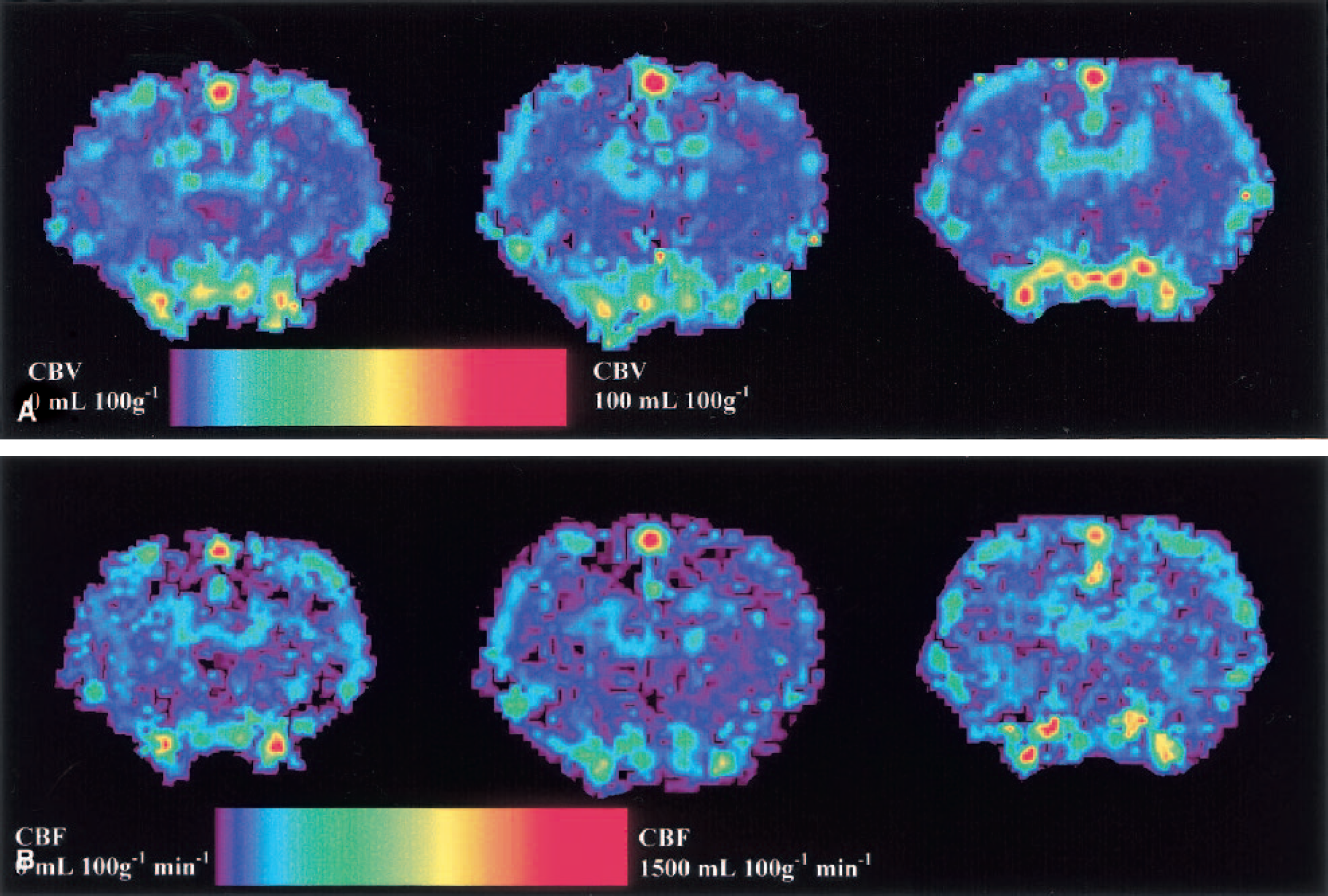
Mean CBV and CBF were computed in five different ROIs: the frontal cortex, the parietal cortex, the caudate putamen, and the whole hemisphere (with and without the blood structures) and in the whole brain (Fig. 6), according to a rat brain atlas (Paxinos and Watson, 1986). All the CBV and CBF results are summarized in Tables 3 and 4. Mean left CBV values of 2.4 ± 0.57, 2.09 ± 0.38, and 2.0 ± 0.38 mL/100 g were found in the frontal cortex, the parietal cortex, and in the caudate putamen, respectively. The global CBV calculated on the whole brain including the blood structures was 4.18 ± 1.06 mL/100 g. Mean left CBF was 154 ± 19, 129 ± 9, and 125 ± 17 mL · 100 g^–1 · min^–1 in the frontal cortex, the parietal cortex, and the caudate putamen, respectively. The global CBF calculated on the whole brain including the blood structures was 215 ± 47 mL · 100 g^–1 · min^–1.

TABLE 3.

Cerebral blood volume measurements of healthy rats in different regions of interest

	Rat no.
	1	2	3	4	5	6	7
	Rat weight
	190	240	240	240	240	240	326
ROI				CBV (mL · 100 g–1)				mean CBV ± SD (mL · 100 g–1)
Frontal cortex, left	2.71	2.68	2.37	3.03	1.92	2.89	1.46	2.44 ± 0.57
Frontal cortex, right	2.63	2.41	2.28	3.18	2.22	2.99	1.41	2.44 ± 0.58
Parietal cortex, left	2.20	2.27	2.20	2.36	1.79	2.42	1.37	2.09 ± 0.38
Parietal cortex, right	2.15	2.33	2.23	2.18	1.96	2.40	1.46	2.10 ± 0.32
Caudate putamen, left	1.96	1.99	2.18	2.50	1.70	2.32	1.37	2.00 ± 0.38
Caudate putamen, right	2.02	1.93	2.30	2.60	1.59	2.38	1.29	2.02 ± 0.46
Brain hemisphere (without blood structures), left	1.99	1.87	2.04	2.16	2.07	2.11	1.24	1.92 ± 0.32
Brain hemisphere (without blood structures), right	1.89	1.80	2.13	2.37	1.92	2.04	1.24	1.91 ± 0.35
Brain hemisphere (with blood structures), left	4.16	3.56	4.58	5.18	3.51	4.20	2.39	3.94 ± 0.89
Brain hemisphere (with blood structures), right	5.55	3.57	3.52	6.26	4.76	4.64	2.10	4.34 ± 1.40
Whole brain	4.93	3.57	4.32	5.57	4.28	4.38	2.22	4.18 ± 1.06

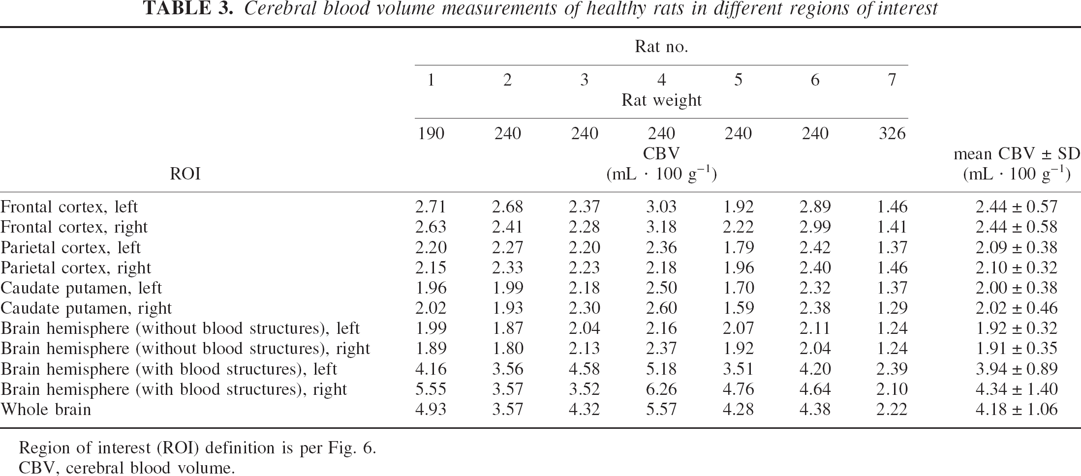
Region of interest (ROI) definition is per Fig. 6.

CBV, cerebral blood volume.

TABLE 4.

Cerebral blood flow measurements of healthy rats in different regions of interest

	Rat no.
	1	2	3	4	5	6	7
	Rat weight
	190	240	240	240	240	240	326
ROI				CBF (mL · 100 g–1 · min–1)				mean CBF ± SD (mL · 100 g–1 · min–1)
Frontal cortex, left	140.30	158.60	175.47	130.44	181.61	144.00	148.02	154 ± 19
Frontal cortex, right	170.30	162.30	153.92	122.05	135.60	150.20	136.51	147 ± 17
Parietal cortex, left	120.60	140.60	131.76	138.71	115.39	134.90	126.43	129 ± 9
Parietal cortex, right	130.40	120.80	126.62	169.17	115.61	113.10	128.90	129 ± 19
Caudate putamen, left	112.60	112.60	148.04	137.28	140.58	103.50	121.48	125 ± 17
Caudate putamen, right	119.10	124.00	142.04	150.19	142.48	102.00	103.79	126 ± 19
Brain hemisphere (without blood structures), left	100.10	100.10	152.58	158.25	123.69	103.50	128.61	124 ± 24
Brain hemisphere (without blood structures), right	110.20	110.20	149.76	194.66	137.24	123.70	124.24	136 ± 30
Brain hemisphere (with blood structures), left	244.90	164.40	223.23	232.41	243.59	179.50	158.29	207 ± 38
Brain hemisphere (with blood structures), right	271.80	148.50	265.23	280.30	239.91	226.50	142.98	225 ± 57
Whole brain	264.10	151.30	251.76	245.21	239.69	194.70	156.49	215 ± 47

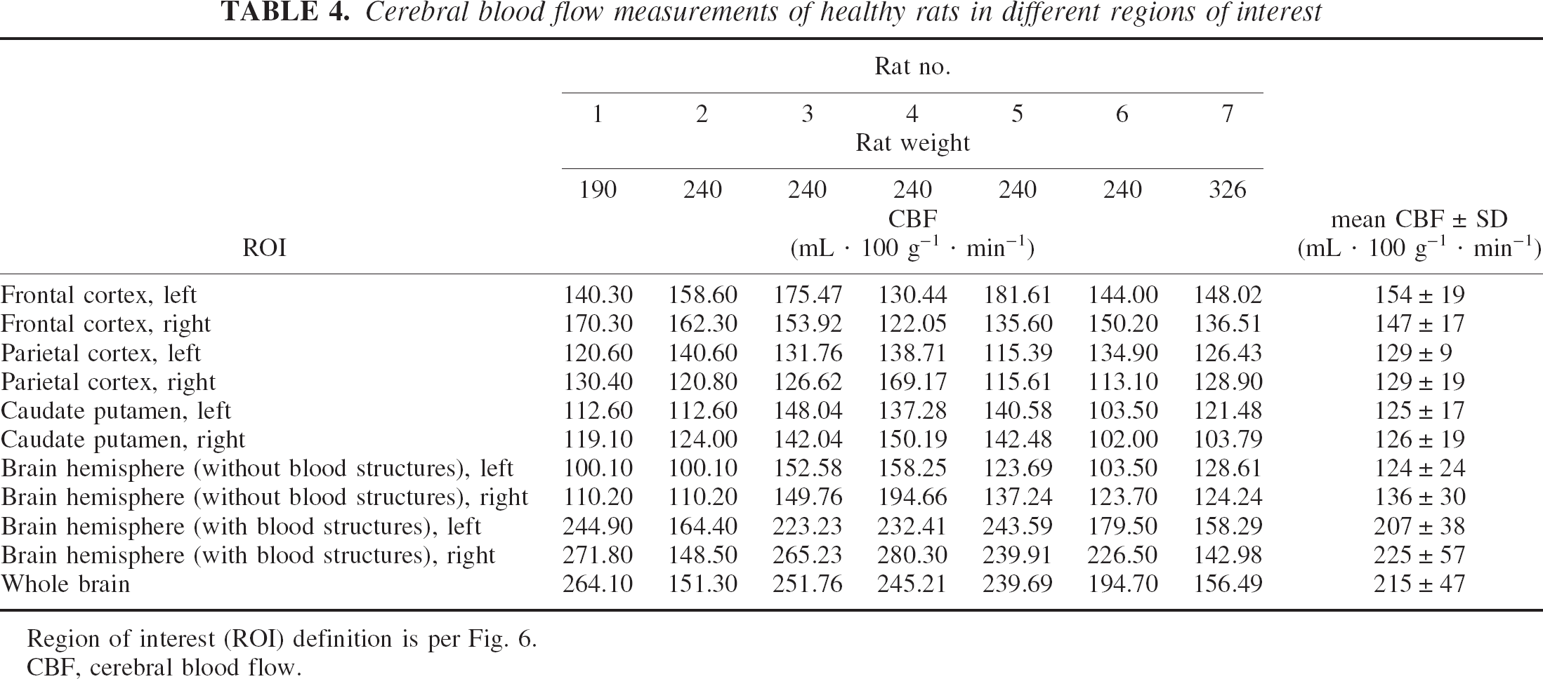
Region of interest (ROI) definition is per Fig. 6.

CBF, cerebral blood flow.

DISCUSSION

The aim of this study was to show that the SRCT technique is reliable and one of the most accurate in vivo methods for the measurement of brain perfusion parameters when compared with the existing methods (MRI, PET scan, or conventional CT), which exhibit many difficulties in quantifying CBV and CBF on an absolute scale.

Such quantification with MRI methods stands only under several conditions. Magnetic susceptibility techniques for quantifying the CBV are based on the hypothesis of a linear relation between the variation of the transverse relaxation rate ΔR₂* and the contrast-agent concentration or the blood volume itself (Kiselev and Posse, 1999; Yablonskiy and Haacke, 1994). These hypotheses stand only for small blood volumes and low contrast-agent concentrations (Barbier et al., 2001; Boxerman et al., 1995). Thus, the presence of high-blood-volume areas (e.g., big vessels, highly perfused regions) induces errors in the CBV values. PET is used for CBV and CBF in vivo measurements (Huang et al., 1983; Phelps et al., 1982; Ter Pogossian and Herscovitch, 1985) but offers a limited spatial resolution (Spinks et al., 2000), leading to important partial volume effects and systematic errors in absolute functional parameters assessment (Iida et al., 2000). Moreover, the very short half-life of the radioisotopes requires the proximity of a cyclotron.

Absolute CBV and CBF measurements with x-ray techniques are directly dependent on the capability to measure in vivo with high precision and accuracy the concentration of an intravascular tracer, thus enabling the use of tracer kinetic theory. In conventional CT scanners, the quantitative assessment of the CBV and CBF (xenon or dynamic CT) relies on the assumption that a linear relation exists between the Hounsfield units and the tracer blood concentration (Axel, 1980; Jaschke et al., 1987; Lee et al., 1990). This condition is not fulfilled with a conventional x-ray generator. The limits of conventional CT scanners in quantifying absolute attenuation coefficients, and thus absolute contrast-agent concentrations in tissues, are mainly due to the broad energy spectrum used, inducing beam-hardening effects. The beam-hardening effect can be partially corrected with an a priori knowledge of the bone or iodine compartment (Joseph and Ruth, 1997). Scattered radiation is another source of error. Numerous correction methods have been proposed with their own limitations (Vetter and Holden, 1988).

Synchrotron radiation, providing monochromatic and intense X-rays, is the alternative fulfilling all the required conditions for accurate quantitative contrast-agent concentration measurements. The x-ray beam monochromaticity is the key issue avoiding beam-hardening effects. The nearly parallel geometry of the fan beam allows the detector to be located far behind the imaged sample to eliminate the scattered beam detection (Dilmanian, 1992; Thomlinson et al., 2000).

Monochromatic CT performances, in terms of accuracy and precision, are fully determined in Dilmanian et al. (1997) and Elleaume et al. (2002). The accuracy of the measurements depends on several variables, mainly on the beam energy, the x-ray dose or photon flux, the contrast-agent concentration, the overall size of the imaged object and the size of the measurement site. The simulations performed in this study on rat head geometry show a precision of 10 μg/mL^–1, and a relative error lower than 2.5% with 5 cGy and 0.5-mm slice thickness. In the case of temporal subtraction at 50 keV on an human head phantom, simulations and experimental measurements show an achievable precision close to 30 μg/mL^–1 and a relative error lower than 3% (concentration range: 0.2–10 mg/mL, skin entrance dose: 20 cGy; slice thickness: 3 mm). With a lower precision (60 μg/mL), the skin entrance x-ray dose delivered for monochromatic SRCT human studies (50 keV, 3-mm slice thickness, relative error <3%) can be reduced to 5 cGy/image, similar to the conventional head CT scan dose delivery of 3 to 7 cGy per slice (Nickoloff and Alderson, 2001). Since 15 to 20 images are necessary for an efficient temporal sampling, the skin entrance dose would range between 0.75 to 1 Gy per examination. The limitations of the synchrotron technique are mainly due to the beam geometry. The source is fixed and therefore the rotation of the imaged sample is required, which could be a problem for patient imaging.

The small size of the imaged structures in this study is challenging because of the detector resolution, implying the correction of the partial volume effects to obtain the CBV and CBF. The correction method that has been used is derived from the one described in Cenic et al. (1999) and has been characterized in this study in terms of dependence on the concentration, on the sampling ROI size, and on the artery size. Reliable CBV and CBF measurements are achievable after correction of the partial volume effects when one selects the biggest brain artery as the arterial input with a 2-pixel-radius ROI to measure the iodine concentrations. If the highest-intensity pixel is used, the correction of the partial volume effects is less efficient. This correction has its own limitation linked to the difficulty of measuring in vivo the artery diameter. This phenomenon decreases the accuracy of SRCT for brain perfusion assessment on small animal models. In the case of larger animal models or human studies, however, the problem is far less critical.

The deconvolution technique used for the CBF computation also affects its precision, since the deconvolution process is very sensitive to noise. There are two major approaches: the Fourier transform approaches (Gobbel and Fike, 1994; Rempp et al., 1994; Smith et al., 2000) and the matrix inversion approach with the singular value decomposition in particular (Ostergaard et al., 1996). The performance of these techniques is still controversial. The parametric Fourier transform method has been used in this article.

Table 5 summarizes several reported values of CBV and CBF and compares them with the ones found with SRCT in the same regions, and mentions the methods used to achieve the CBV and CBF estimation. The CBV values found in literature lead to controversies and slightly depend on the method that is used, in particular for the autoradiographic techniques where blood fixation may be performed. Todd et al. (1993) reported that autoradiography without any fixation gives CBV values that are always lower than those obtained with microwave fixation. If no fixation is performed, the blood pressure falls to zero, leading to a lower CBV. The SRCT values, however, are close to the CBV values measured by autoradiography with blood fixation or MRI.

TABLE 5.

Comparison of rat brain synchrotron radiation computed tomography cerebral blood volume and blood flow with the literature values

Region of interest	Method	Reference (for our study n = 7)	CBV ± SD (mL · 100 g–1)	CBF ± SD (mL · 100 g–1 · min–1)
Caudate putamen	SRCT	Our study	1.92 ± 0.32	125 ± 17
	Autoradiography	Cremer and Seville, 1983	0.63 ± 0.01	123 ± 7
	Autoradiography	Nakagawa et al., 1995	0.69 ± 0.02	—
	Autoradiography	Bereczki et al., 1993b	0.85 ± 0.04	130 ± 17
	In vivo MRI	Payen et al., 2000	2.94 ± 0.43	—
	In vivo MRI	Troprès et al., 2001	2.87	—
Frontal cortex	SRCT	Our study	2.44 ± 0.58	150 ± 18
	Autoradiography	Bereczki et al., 1993b	1.05 ± 0.05	170 ± 25
	Autoradiography	Cremer and Seville, 1983	0.95 ± 0.04	142 ± 7
	Autoradiography	Nakagawa et al., 1995	0.83 ± 0.02	—
Parietal cortex	SRCT	Our study	2.1 ± 0.38	129 ± 18
	In vivo optical method	Shockley and LaManna, 1988	3.4 ± 0.4	144 ± 14
	Autoradiography	Nakagawa et al., 1995	0.99 ± 0.04	—
Whole cortex	SRCT	Our study	2.05 ± 0.4	140 ± 18
	Autoradiography with blood fixation	Aizawa et al., 1990	2.88 ± 0.56	144 ± 14
	In vivo MRI	Schwarzbauer et al., 1997	1.63 ± 0.18	—
	In vivo MRI	Payen et al., 2000	3.01 ± 0.43	—
	In vivo MRI	Troprès et al., 2001	4.07	—
Brain hemisphere	SRCT	Our study	1.92 ± 0.32	130 ± 25
without large vessels	Autoradiography with blood fixation	Everett et al., 1956	2.88 ± 0.8	—
	In vivo MRI	Lin et al., 1999	2.96 ± 0.8	—
Whole brain	SRCT	Our study	4.18 ± 1.06	215 ± 47
	Autoradiography with blood fixation	Todd et al., 1993b	2.67 ± 0.33	101 ± 24
	Autoradiography with blood fixation	Todd et al., 1993a	2.96 ± 0.57	127 ± 22

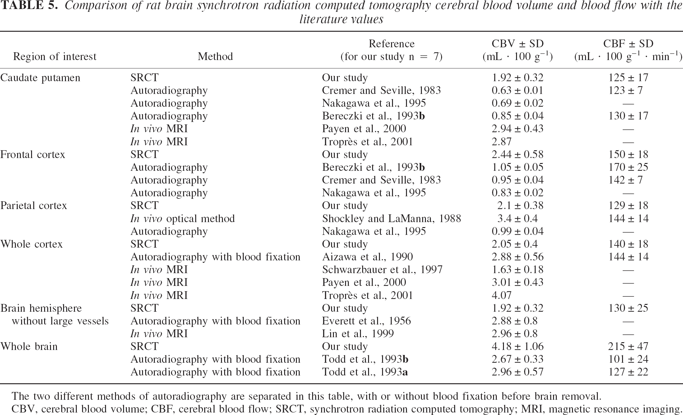
The two different methods of autoradiography are separated in this table, with or without blood fixation before brain removal.

CBV, cerebral blood volume; CBF, cerebral blood flow; SRCT, synchrotron radiation computed tomography; MRI, magnetic resonance imaging.

Until now only few quantitative CBV or CBF values have been obtained in vivo with the healthy rat model (Lin et al., 1999; Payen et al., 2000; Schwarzbauer et al., 1997; Shockley and LaManna, 1988; Troprès et al., 2001). Previously reported CBV measurements on dogs (Nabavi et al., 1999a, b ) or rabbits (Cenic et al., 1999, 2000) with dynamic CT show CBV values for the grey matter close to 2 mL/100 g, similar to the values found in this study.

For the CBF measurements, the SRCT values are in good agreement with those reported in the literature. The CBF values for a given brain region are less dependent on the technique used (Table 5). The SRCT CBF values are consistent with the commonly reported ones in all the ROIs, except for the whole-brain ROI since major vessels contribute to the SRCT CBF measurements, which is not the case for other techniques. The same problem occurs for the CBV measurements.

To our knowledge, this is the first report of the in vivo assessment of the CBV and the CBF using monochromatic x-rays. SRCT is a new tool for the study of cerebral physiopathology hemodynamic changes, such as those observed in brain tumors or in cerebrovascular diseases, and the method developed in this article could be particularly useful in the domain of novel attempts to treat brain tumors by inducing changes in brain perfusion. Various modalities of radiation therapy using synchrotron radiation (Corde et al., 2002; Dilmanian et al., 2002; Laissue et al., 1998) are under active development in different synchrotron facilities, including the ESRF. The possibility of assessing brain perfusion reinforces the potential of these programs.