Sage Journals: Discover world-class research

Abstract

One of the most limiting factors for the accurate quantification of physiologic parameters with positron emission tomography (PET) is the partial volume effect (PVE). To assess the magnitude of this contribution to the measurement of regional cerebral blood flow (rCBF), the authors have formulated four kinetic models each including a parameter defining the perfusable tissue fraction (PTF). The four kinetic models used were 2 one-tissue compartment models with (Model A) and without (Model B) a vascular term and 2 two-tissue compartment models with fixed (Model C) or variable (Model D) white matter flow. Furthermore, rCBF based on the autoradiographic method was measured. The goals of the study were to determine the following in normal humans: (1) the optimal model, (2) the optimal length of fit, (3) the model parameters and their reproducibility, and (4) the effects of data acquisition (2D or 3D). Furthermore, the authors wanted to measure the activation response in the occipital gray matter compartment, and in doing so test the stability of the PTF, during perturbations of rCBF induced by visual stimulation. Eight dynamic PET scans were acquired per subject (n = 8), each for a duration of 6 minutes after IV bolus injection of H₂¹⁵O. Four of these scans were performed using 2D and four using 3D acquisition. Visual stimulation was presented in four scans, and four scans were during rest. Model C was found optimal based on Akaike's Information Criteria (AIC) and had the smallest coefficient of variance after a 6-minute length of fit. Using this model the average PVE corrected rCBF during rest in gray matter was 1.07 mL·min⁻¹·g⁻¹ (0.11 SD), with an average coefficient of variance of 6%. Acquisition mode did not affect the estimated parameters, with the exception of a significant increase in the white matter rCBF using the autoradiographic method (2D: 0.17 mL·min⁻¹·g⁻¹ (0.02 SD); 3D: 0.21 mL·min⁻¹·g⁻¹ (0.02 SD)). At a 6-minute fit the average gray matter CBF using Models C and D were increased by 100% to 150% compared with Models A and B and the autoradiographic method. There were no significant changes in the perfusable tissue fraction by the activation induced rCBF increases. The largest activation response was found using Model C (median = 39.1%). The current study clearly demonstrates the importance of PVE correction in the quantitation of rCBF in normal humans. The potential use of this method is to cost-effectively deliver PVE corrected measures of rCBF and tissue volumes without reference to imaging modalities other than PET.

Keywords

Positron emission tomography Regional cerebral blood flow Partial volume effect Visual cortex Activation

Using ¹⁵O-water in positron emission tomography (PET) provides a method for in vivo quantification of regional cerebral blood flow (rCBF) (Kanno et al., 1987; Raichle et al., 1983). It is well known that the obtained quantitative values of rCBF using the autoradiographic (ARG) method and PET are systematically underestimated because of the so-called partial volume effect (PVE) (Iida et al., 1999), which is among the most important limiting factors for accurate quantification. Until recently methods for PVE correction have been primarily performed with reference to structural imaging techniques, CT or MRI (see Labbe et al., 1996)). An alternative approach is to formulate kinetic models in which a term for the perfusable tissue fraction (PTF, α) is included, a method which has previously been used successfully for PET quantification of myocardial blood flow (Iida et al., 1988b,1991,1995). The PTF is defined as the fractional mass of the tissue that is capable of rapidly exchanging water within a region of interest (ROI) and is expressed in g/mL as the ratio of this mass to the ROI volume.

The authors have transferred this principle to four kinetic model configurations of the dynamic behavior of ¹⁵O-water in the brain, all correcting rCBF using the PTF (Iida et al., 1999). The four models were initially implemented, compared, and validated on data derived from the brains of macaque monkeys. The models were framed as 2 one-tissue compartment models with (A) and without (B) a vascular term and two two-tissue compartment models with a white matter flow that was either fixed at 0.20 mL·min⁻¹·g⁻¹ (C) or variable (D). The gray matter rCBF was increased by approximately 100% using the optimal model (C) compared with values from assumed gray matter regions using the ARG method.

The object of the current study was to apply the same four models and the ARG method to normal humans and determine the optimal model, the optimal length of fit within a 6-minute acquisition period, the model parameters and reproducibility, and the effects of data acquisition (2D or 3D). Furthermore, the authors wanted to measure the activation response in the occipital gray matter compartment during perturbations of rCBF induced by visual stimulation after PTF correction had been performed. Based on the findings from the monkey data the a priori expectations were that the estimated gray matter rCBF values using the optimal model would be approximately 100% larger than the ARG method. The authors also considered the possibility that the activation response measured as percent of a baseline resting condition would be increased. A larger activation response would depend on the composition of gray and white matter in a given ROI and implicitly assumes that the white matter tissue compartment either does not react to or reacts less to visual stimulation. It furthermore follows from the models that the estimated PTF within a ROI should remain constant regardless of changes in rCBF.

METHODS

Subjects

Subjects consisted of eight strongly right-handed paid healthy volunteers (median age = 23 years; range 21 to 26 years; 4 female, 4 male). None of the subjects had past or present neurologic or psychiatric disorders or active use of medication or recreational drugs. Informed consent was obtained according to the Declaration of Helsinki II, and the study was approved by the local ethics committee of Copenhagen (J. nr. (KF) 01-196/97).

Experimental design

Eight scans were performed per subject divided between three within-subject factors: acquisition, 2D or 3D mode; behavioral state, resting or visual stimulation; and repeat, first or second scan. For practical reasons the two acquisition modes were performed in balanced blocks of four scans with either 2D before 3D or reversed. Within each block the subjects were scanned in two resting and two stimulation conditions in randomized order. Thus, the design was a complete within-subject design with all subjects measured on all independent variables.

PET scanning

Head movements were limited by head-holders constructed by moulded foam, and a 10-minute transmission scan was performed for attenuation correction. A short indwelling catheter was placed in the left nondominant radial artery for blood sampling.

Positron emission tomography scans were obtained with an 18 ring GE-Advance scanner (General Electric Medical, Milwaukee, WI, U.S.A.) operating in either 2D or 3D acquisition mode producing 35 image slices with an interslice distance of 4.25 mm. The total axial field of view was 15.2 cm with an approximate in-plane resolution of 5 mm. Technical specifications have been described elsewhere (DeGrado et al., 1994; Lewellen et al., 1996).

During reconstruction the images were corrected for randoms and scatter (Stearns, 1995), decay, detector efficiency variations, and dead time. They were reconstructed with an 8.0-mm Hanning filter transaxially and the 3D images were additionally filtered axially with an 8.5-mm Ramp filter.

Oxygen-15-labeled water was administered by hand as a 5 mL bolus into an antecubital intravenous catheter in the right arm over 3 to 5 seconds immediately followed by 10 mL of physiologic saline for flushing. To approximately match the 2D and 3D acquisitions for sensitivity, the injected doses were 1 GBq (27 mCi) and 0.2 GBq (5.4 mCi), respectively. The effective dose was calculated to 6.0 mSv (Smith et al., 1994), and larger doses could not be applied because of ethical considerations. The interinjection intervals were 10 to 31 minutes (average 14.3 minutes), but 28 to 54 minutes (average 35.5 minutes) when switching from 2D to 3D acquisition mode.

Arterial blood sampling was initiated 30 seconds before isotope injection and dynamic imaging began 10 seconds after injection. Dynamic scans were obtained over 6 minutes with frame durations of 12 × 5 seconds, 8 × 15 seconds, and 6 × 30 seconds in 2D; and 12 × 5 seconds, 4 × 15 seconds, 4 × 30 seconds, and 2 × 60 seconds in 3D. This difference was caused by computer memory limitations on the demanding 3D acquisition.

Radioactivity concentration in the arterial blood was continuously monitored by an automatic blood sampling system (ABSS) by withdrawal of blood between two pairs of BGO crystals in a coincidence circuit (Advance Fluid Radioactivity Quantifier System, GE). The detectors in the ABSS were cross-calibrated against the PET scanner and the sampling frequency was 1 Hz. The inner diameter of the tube connected to the arterial catheter was 1.2 mm and the flow rate was 4.0 mL/min. Because of the length of scanning and the number of scans performed, the authors chose to reduce the flow rate from the usual 8.0 mL/min, thus limiting the total blood loss to approximately 250 mL. The arterial input curves were corrected for decay and delay, and dispersion correction was performed according to previously reported procedures involving deconvolution and nonlinear least-squares fitting (Iida et al., 1988a,1986). Arterial blood partial pressures of O₂ (P_ao₂) and CO₂ (P_aco₂) and hematocrit values were measured immediately after each PET scan (ABL system 510, Radiometer, Copenhagen, Denmark).

The activation paradigms were rest with eyes closed or visual stimulation by a reversing annular checkerboard at 8 Hz displayed on a computer screen. The subjects were told to focus attention at the center of the annulus. This paradigm is well characterized and widely used in methodologic evaluations to provide large, focal, and reproducible activations of 20% to 40% in visual cortex (Belliveau et al., 1991; Fox and Raichle, 1984,1985; Vafaee et al., 1999). Stimulation was initiated at 2 minutes before isotope injection and continued throughout the acquisition period. Both conditions were performed in a dimmed and quiet room.

MRI scanning

Structural MRI scanning was performed with a 1.5 T Vision scanner (Siemens, Erlangen, Germany) using a 3D MPRAGE sequence (repetition time/echo time/inversion time = 11/4/300 milliseconds, flip angle 12°). The images were acquired contiguously in the sagittal plane with an inplane resolution of 0.92 mm, and a slice thickness 1.0 mm. The number of planes was 170 and the in-plane matrix dimensions were 256 × 256.

Image processing and regions of interest

Taking into account head movements between scan sessions the 6-minute summed intrasubject images were aligned on a voxel-by-voxel basis using a three-dimensional automated six parameters rigid body transformation (Automated Image Registration (AIR) software, version 3.0; Woods et al., 1992). The transformation parameters derived from this process were used to realign the individual time frames in the respective dynamic scans. The 90-second ARG rCBF images were calculated through time frame summation (Kanno et al., 1987). These images were subsequently used for calculation of the single subject activation response using Statistical Parametric Mapping software (SPM-96; Wellcome Department of Cognitive Neurology, London, U.K.; Frackowiak and Friston, 1994). Differences in global blood flow were removed by proportional normalization to a value of 0.50 mL·min⁻¹·g⁻¹. When comparing visual stimulation to rest, the activated regions were defined as the voxels of a continuous cluster located in the occipital region above a significance threshold level of P < 0.05, uncorrected for multiple comparison. Two 3D ROIs were drawn manually covering several slices, a visual ROI that encompassed the above defined region, and a global ROI of all tissue from the centrum semiovale and above the visual ROI (Fig. 1). To assure that all cortical gray matter counts were sampled, the outer boundaries of the ROIs were placed approximately 15 mm from the cortical edge. These ROIs were then projected onto the dynamic images across conditions to generate regional time-activity curves (TACs) for all time frames.

FIG 1.

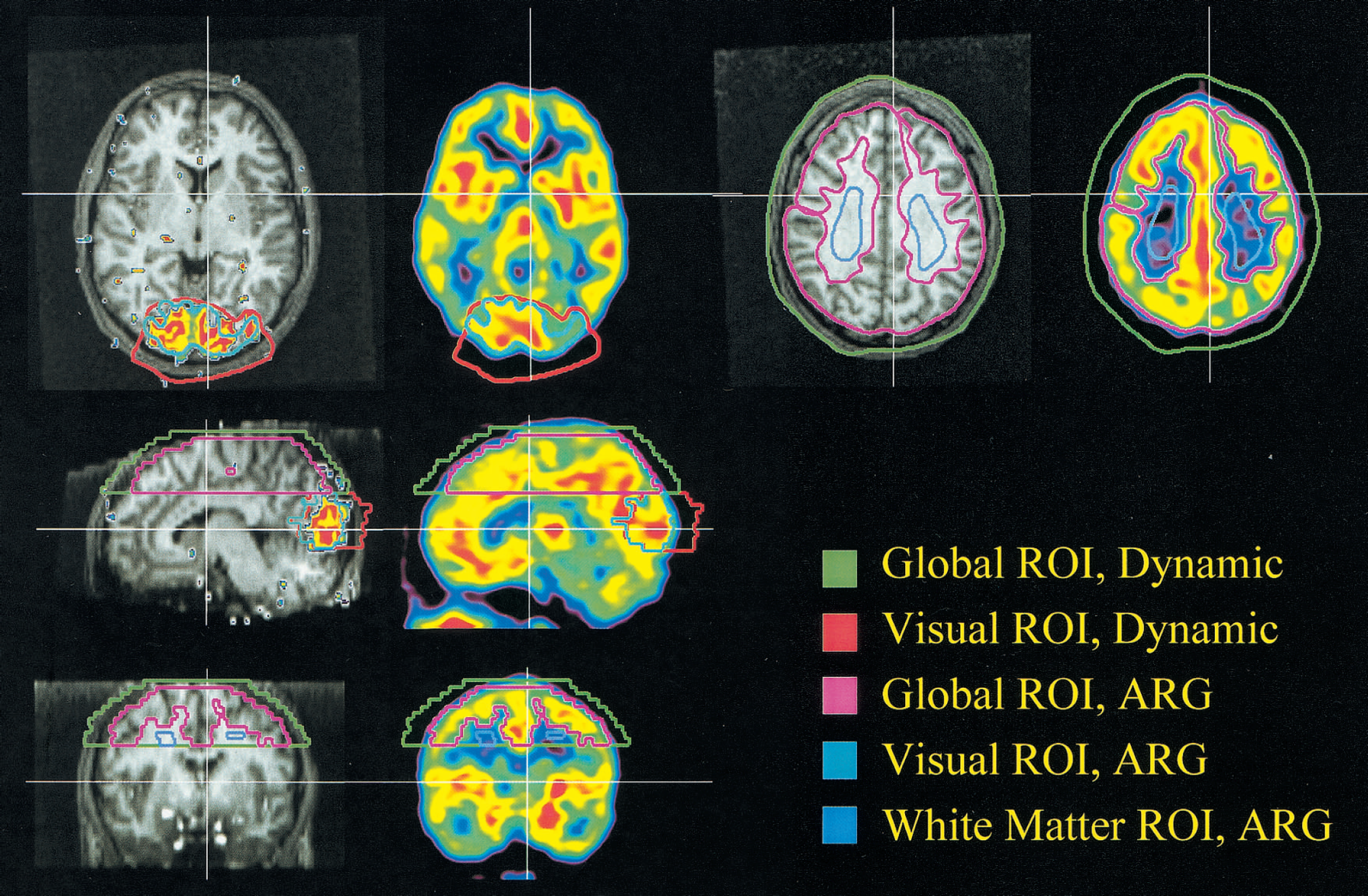
Configuration of visual, global, and white matter (autoradiographic only) regions of interest (ROIs) applied using either dynamic fitting or the autoradiographic method. The five ROIs are superimposed on a positron emission tomography autoradiographic regional cerebral blood flow (rCBF) image from a single subject and the corresponding coregistered T1-weighted magnetic resonance image with the significantly activated area (P < 0.05) during visual stimulation projected on top. Coronal, sagittal, and two transaxial views (top) are shown.

Separate visual and global ROIs were manually drawn on the ARG rCBF images with reference to the aligned structural MRI scan. The intention was to cover only the gray matter regions at the same time minimizing the contribution from white matter and extracerebral tissues. These were thus placed on the same slices as and within the dynamic visual and global ROIs. An additional ROI was placed in the centrum semiovale in representative white matter as defined on the structural MRI scan (Fig. 1).

Fitting procedure

Time-activity curves were fitted using four different models as previously described (Iida et al., 2000). These comprise a single tissue compartment model (A), a single tissue compartment model with an arterial blood volume component (B), and two gray and white two-tissue parallel compartment models (C and D):

R (t) = α \cdot f \cdot C_{a} (t) \otimes e^{- \frac{f}{p} t}

(A)

R (t) = (1 - V_{a}) \cdot α \cdot f \cdot C_{a} (t) \otimes e^{- \frac{f}{p} t} + V_{a} \cdot C_{a} (t)

(B)

R (t) = α_{g} \cdot f_{g} \cdot C_{a} (t) \otimes e^{- \frac{f_{g}}{p_{g}} t} + α_{w} \cdot f_{w} \cdot C_{a} (t) \otimes e^{- \frac{f_{w}}{p_{w}} t}

(C,D)

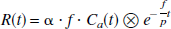
where R(t) and C_a(t) are the decay corrected cerebral and arterial time-activity curves, respectively, measured in Bq/mL. In Model A, f is the average tissue mass rCBF (mL·g⁻¹·min⁻¹), and f_g and f_w are the fitted rCBF values (mL·g⁻¹·min⁻¹) for gray and white matter, respectively. Likewise, α represents the total PTF (g/mL), whereas α and α_w are the PTFs (g/mL) specifically for gray and white matter. The average brain tissue-to-blood partition coefficient of water, p, is fixed at 0.9 mL/g, whereas the corresponding parameters for gray and white matter, p_g and p_w are fixed at 1.0 mL/g and 0.8 mL/g, respectively (Herscovitch and Raichle, 1985). ⊗ denotes the convolution operation. Model B is formulated according to Ohta et al. (1996), thus V_a represents the arterial blood volume (mL/mL). Evidently, the only difference between Models A and B is the inclusion of the arterial blood volume term. The difference between Model C and D is that the white matter rCBF, f_w, is fixed at 0.20 mL·min⁻¹·g⁻¹ in Model C, whereas it is fitted in Model D.

Calculations and statistical evaluation

Model stability

To assess the stability of the models over a range of different fitting time periods, the data included in the fit were systematically increased from 1 to 6 minutes at steps of 1 minute estimating the parameters at each interval. The means, standard deviations, and coefficients of variation (CVs) of the fitted parameters were calculated for each time interval.

Optimal model

At the longest fitting period of 6 minutes the AIC (Akaike, 1974) was calculated to evaluate the optimal model at this time point

A I C = n \cdot \ln (S S Q) + 2 p

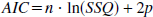
where n is the number of measurements, SSQ is the sum of squares between the model predictions and the measured tissue radioactivity concentration normalized for the variance in R, and p is the number of parameters.

Statistical evaluation

Only the parameters and the AIC values after the full 6-minute fit were used in further statistical analysis. The statistical model used on each fitted and calculated parameter and AIC value was a full interaction repeated measures analysis of variance (ANOVA) model with behavioral state, acquisition, repeat, and model (when more than one) as within factors. Significant main effects of the kinetic model were followed post hoc by 6 two-tailed paired multiple t-tests between all kinetic models with Bonferroni correction at a threshold level of P < 0.05 (t = 2.7, df = 63). As these analyses were biased by data from models that were subsequently rejected, a separated analysis on the optimal kinetic model (C) was performed. A similar ANOVA structure was used for the evaluation of the arterial blood gas measures and the ARG rCBF values.

Furthermore, the authors statistically tested two null hypotheses. The first was whether V_a (B) could be assumed to be 0 mL/mL. The second was whether f_w (D) was equal to the fixed f_w value of 0.2 mL·min⁻¹·g⁻¹ in Model C. A two-tailed Student's t-test at a significance threshold level of P < 0.05 was used.

Estimated tissue volumes

The volumes of gray and white matter were calculated using the optimal model (C, see below) by multiplying the PTFs, α_g and α_w, with the ROI volumes, and dividing by the tissue density (1.04 g/mL).

Reproducibility

As an expression of the reproducibility the intraindividual CV and the interindividual average CVs and standard deviations were calculated for each estimated parameter in Model C and for the ARG values.

Decreasing ROI size will increase noise. To investigate the stability of Model C as a function of ROI size a total of 30 nonoverlapping ROIs were drawn on the first 2D rest condition in every subject and subsequently projected onto the second 2D rest condition. There were 3 different ROI sizes with 10 individual ROIs per size. The smallest ROI size was 300 voxels (5.1 mL), of which approximately 100 voxels in the center constituting presumed gray matter judged from the ARG image. The sizes of the remaining two ROIs were 600 (10.2 mL) and 1200 voxels (20.4 mL) with presumed gray matter contents of 200 and 400 voxels, respectively. Values of each ROI were fitted dynamically using Model C. From these fitted parameters the α_g* f_g product and α_g * f_g + α_w * 0.2 mL·min⁻¹·g⁻¹ product were calculated. For each of the eight subjects, three ROI sizes and five fitted-calulated parameters, the half of the variance of the differences between the two rest conditions was calculated. The intrasubject CVs were expressed as the square root of this term divided by the average of all rest conditions. Finally the average intrasubject CVs for each parameter and ROI size were calculated.

Activation response

To assess the effects of kinetic model on the activation response, the subject specific average activation responses during visual activation (4 scans) were computed in percent of the average resting values (4 scans) in the visual ROIs. This was performed from the estimated flow values, f or f_g, in all four dynamic models and the ARG rCBF data.

The Friedman test, a nonparametric two-way ANOVA by ranks for matched samples, was used to test the null-hypothesis that the activation response in percent was unaffected by the quantitative model. This analysis was followed by multiple post hoc paired signed rank tests (Wilcoxon) between models at an uncorrected threshold level of P < 0.008. These analyses were performed both using the raw quantitative data in the visual ROI and after normalization of the quantitative values in the visual ROI by the values in the global ROI.

RESULTS

Physiologic data

There were no significant differences in the P_aco₂ or P_ao₂ values by the ANOVA, either as main effects or interactions. The main effect of the hematocrit value was significantly (P < 0.05, F_{1, 7} = 9.77) increased by an average of 0.002 during visual stimulation compared with rest (Table 1). The reason for this change is unknown. The effect this perturbation may have on the rCBF values, however, is minimal and can be neglected.

TABLE 1.

Physiologic data

Condition	Hematocrit (%)	P_ao₂ (kPa)	P_aco₂ (kPa)
Rest	0.380 ± 0.063	13.09 ± 0.63	5.12 ± 0.50
Stimulation	0.382 ± 0.063*	13.09 ± 0.59	5.09 ± 0.50

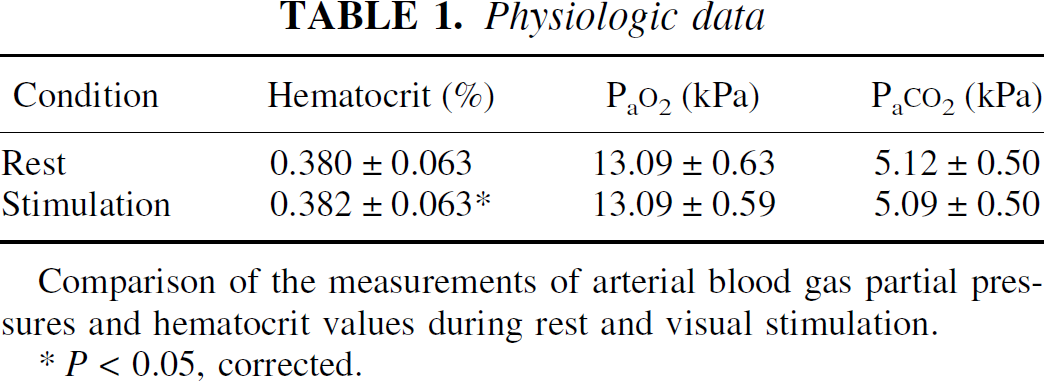
Comparison of the measurements of arterial blood gas partial pressures and hematocrit values during rest and visual stimulation.

P < 0.05, corrected.

Model stability

The effects of kinetic model and fitting time period on rCBF (f, f_g) and the PTF's (α, α_g, α_w) can be seen in Figs. 2 to 4. The steady decrease of f_g values and increase of α_g values with the length of fit using Models A and B, which do not contain terms for f_w and α_w, indicate instability. In Model C, average f, α, and α_g values stabilize after a fitting period of approximately 4 minutes, however a CV improvement can still be gained by prolonging the fit to 6 minutes. For Model D, it is uncertain if the estimated values are stable after a fitting period of 6 minutes. The average values of f_g and α_g are similar to those derived from Model C, however, the variances are significantly larger. Only AIC values and estimated parameters after the full 6-minute fit were used in the ANOVA comparing models because of the instability of Model D at shorter fitting periods.

FIG. 2.

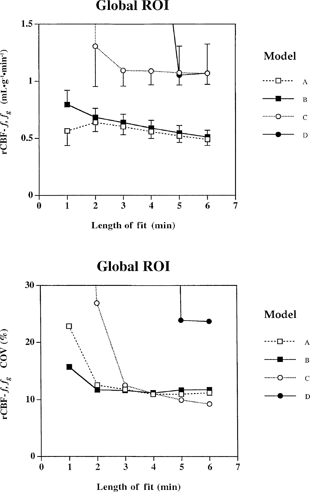
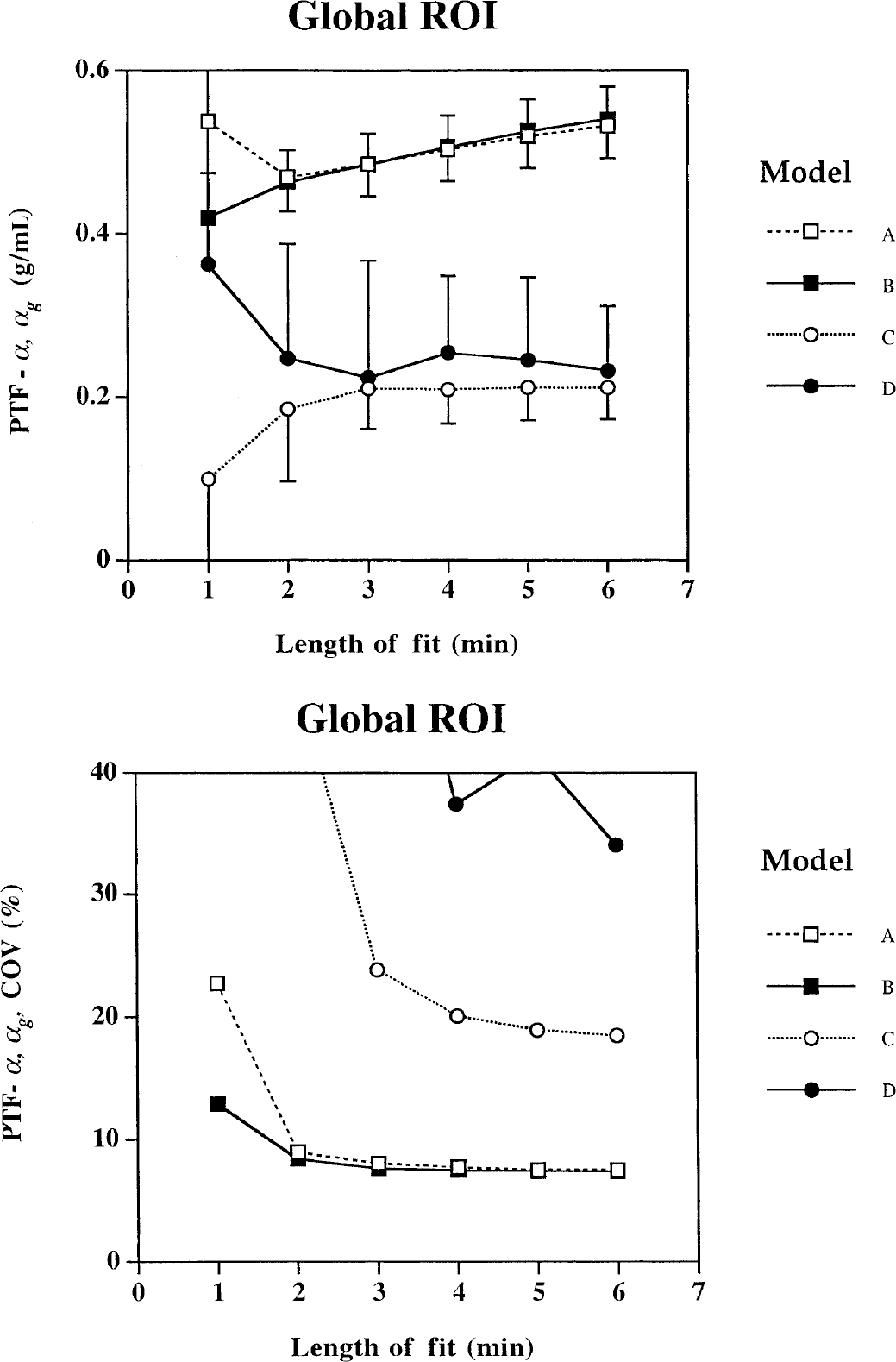
Effects of increasing the length of fitting period on the estimated parameters for the gray matter regional cerebral blood flow (rCBF) acquired from the global regions of interest (ROI). (top) Estimated parameter values using Models A to D and the autoradiographic model are displayed as mean ± SD. (bottom) Corresponding coefficients of variance (CV).

FIG. 3.

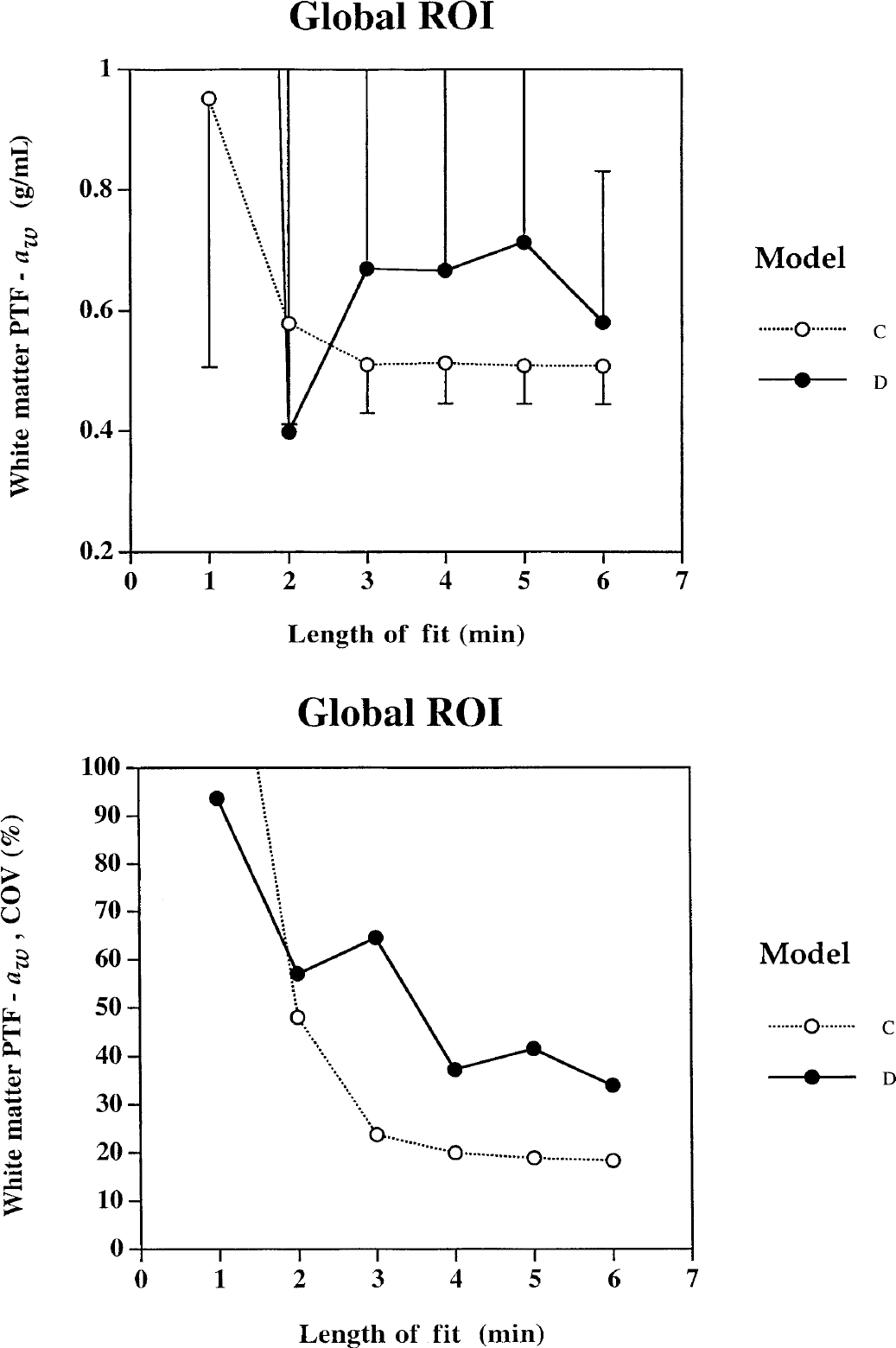
Effects of increasing the length of fitting period on the estimated parameters for the gray matter perfusable tissue fraction acquired from the global regions of interest. (top) Estimated parameter values using Models A to D are displayed as mean ± SD. (bottom) Corresponding coefficients of variance (CV).

FIG. 4.

Effects of increasing the length of fitting period on the estimated parameters for the white matter perfusable tissue fraction (PTF) acquired from the global regions of interest (ROIs). (top) Estimated parameter values using Models C and D are displayed as mean ± SD. (bottom) Corresponding coefficients of variance (CV).

Representative data sampled in the visual ROI with curves fitted by use of the four models appear in Fig. 5. The curve fits obtained by Model C and D are almost identical. Models A and B clearly perform suboptimally particularly during the flow increases of visual stimulation.

FIG. 5.

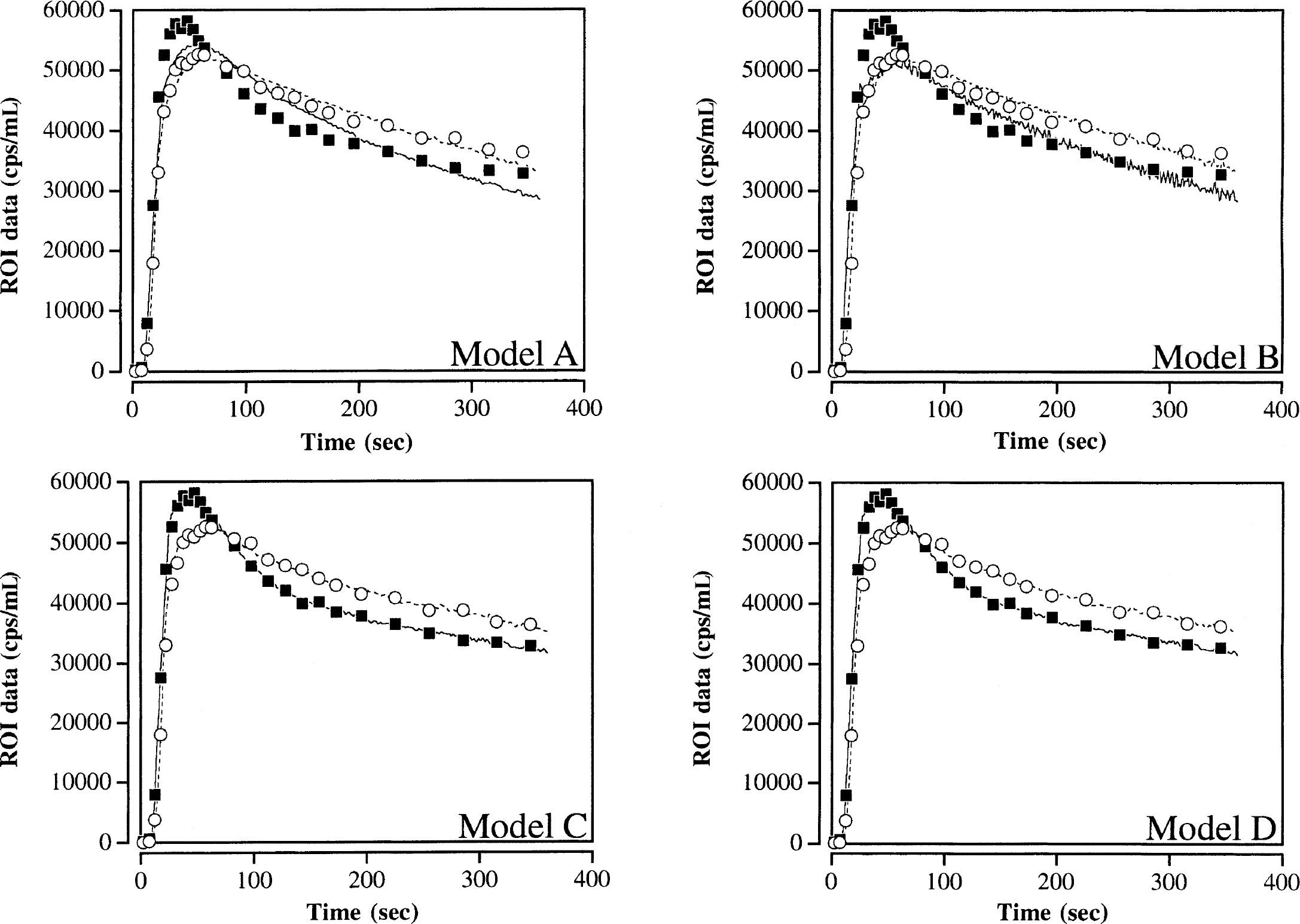
Representative time-activity curves obtained from a single subject in the visual regions of interest (ROI) during rest (○) and full-field visual stimulation (■). Corresponding fitted tissue curves for the full 6-minute time period using 4 different kinetic models are shown. Dotted line represents the fit using the ROI data during rest, whereas the solid line is during visual stimulation. For these data the fitted curves using Model C and D can hardly be distinguished. The data shown was acquired in 2D mode and decay corrected.

Optimal model

Analysis of variance of the AIC values showed significant main effects of the kinetic model for the global and visual ROIs (P < 0.001). The post hoc t-tests had the same results for both ROIs: B > A > C and C = D (Table 2 and 3). As no significant differences in AIC were found between Models C and D, the simpler model (C) was nominated as optimal when the length of fit was 6 minutes.

TABLE 2.

Akaike Information Criteria

Model	Global ROI	Visual ROI
A	602 ± 112	610 ± 119
B	616 ± 111	618 ± 122 *
C	567 ± 110	571 ± 115 * *
D	568 ± 111	573 ± 116 * *

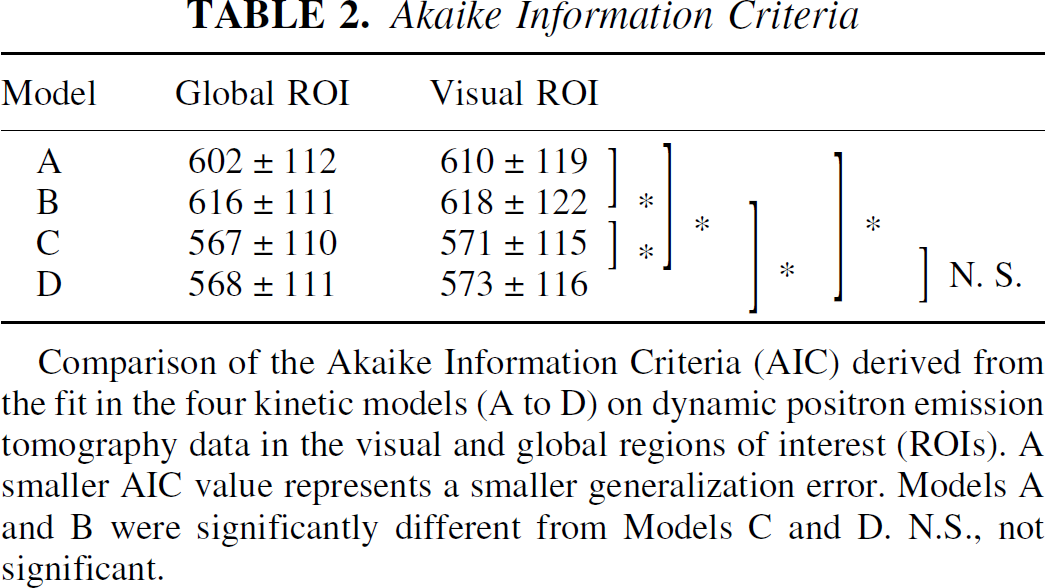
Comparison of the Akaike Information Criteria (AIC) derived from the fit in the four kinetic models (A to D) on dynamic positron emission tomography data in the visual and global regions of interest (ROIs). A smaller AIC value represents a smaller generalization error. Models A and B were significantly different from Models C and D. N.S., not significant.

Effects of acquisition, behavioral state, and repeat on the model parameters

There were no statistically significant differences between Models C and D for f_g and α_g (Tables 3 to 5). Comparing Model B to Model A shows that the f and α values were significantly larger by 4% and 2%, respectively, and the V_a term in Model B was significantly larger than zero (P < 0.001). The f values (A and B) were approximately half of the values for f_g (C and D), and conversely the α values were twice the values for α_g. There were no significant changes of α or α_g as a result of visual stimulation, acquisition, or repeat.

TABLE 3.

Summary of statistical analysis

	Global ROI		Visual ROI
Fitted/calculatedparameter
Fitted/calculatedparameter	Model effect	Other effects	Model effect	Other effects	Model C
AIC	B > A > C = D**	Not evaluated	B > A > C = D**	Not evaluated
f,f_g (mL·g⁻¹·min⁻¹)	A < B < C = D**		A < B < C = D**	State, R < V; Model × State	State**, R < V
α, α_g (g/mL)	B > A > C = D**		B > A > C = **
f_w (mL·g⁻¹·min⁻¹)	D		D
α_W (g/mL)	C < D*		C < D*

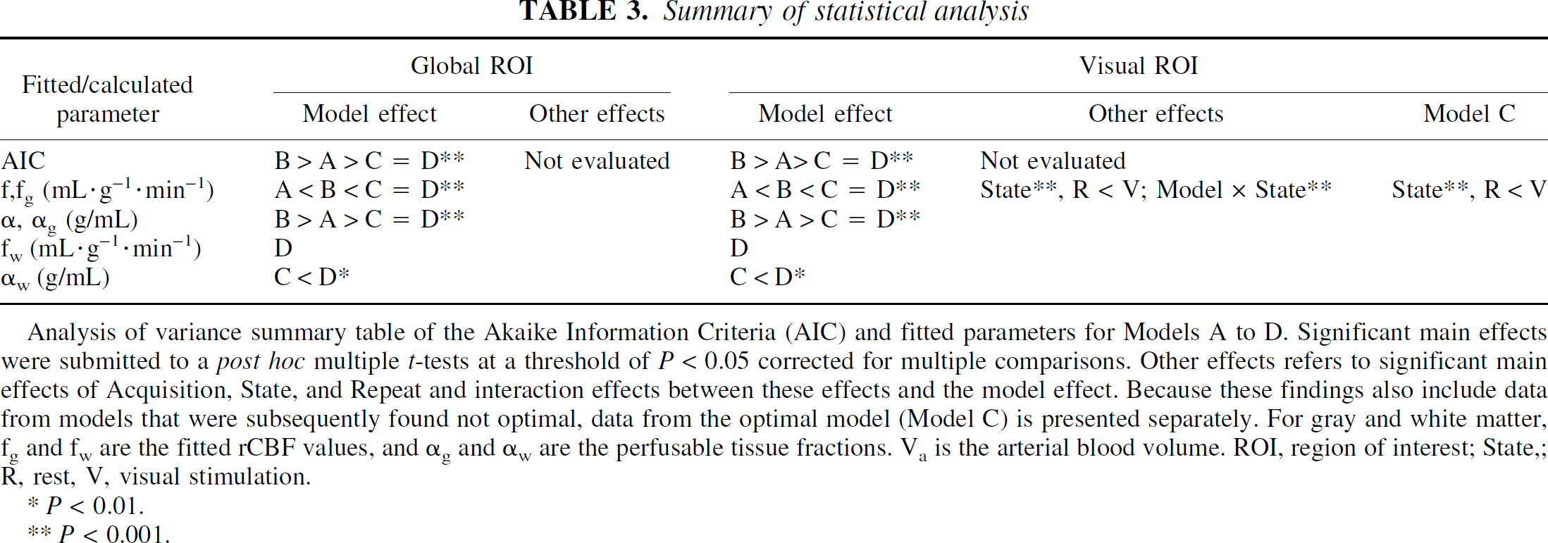
Analysis of variance summary table of the Akaike Information Criteria (AIC) and fitted parameters for Models A to D. Significant main effects were submitted to a post hoc multiple t-tests at a threshold of P < 0.05 corrected for multiple comparisons. Other effects refers to significant main effects of Acquisition, State, and Repeat and interaction effects between these effects and the model effect. Because these findings also include data from models that were subsequently found not optimal, data from the optimal model (Model C) is presented separately. For gray and white matter, f_g and f_w are the fitted rCBF values, and α_g and α_w are the perfusable tissue fractions. V_a is the arterial blood volume. ROI, region of interest; State,; R, rest, V, visual stimulation.

P < 0.01.

P < 0.001.

TABLE 4.

Comparison of fitted parameters from four different kinetic models on dynamic PET data in the global ROI

Condition	Model	f, f_g (mL·min⁻¹·g⁻¹)	α, α_g (g/mL)	f_w (mL·min⁻¹·g⁻¹)	α_W (g/mL)	V_a (mL/mL)
Rest	A	0.50 ± 0.06	0.53 ± 0.04	–	–	–
	B	0.52 ± 0.07	0.54 ± 0.04	–	–	0.012 ± 0.005
	C	1.07 ± 0.11	0.21 ± 0.04	0.20 (fixed)	0.51 ± 0.06	–
	D	1.05 ± 0.23	0.24 ± 0.09	0.17 ± 0.08	0.62 ± 0.34	–
Stimulation	A	0.49 ± 0.05	0.53 ± 0.04	–	–	–
	B	0.51 ± 0.05	0.54 ± 0.04	–	–	0.013 ± 0.004
	C	1.07 ± 0.08	0.21 ± 0.04	0.20 (fixed)	0.51 ± 0.07	–
	D	1.10 ± 0.27	0.22 ± 0.07	0.18 ± 0.07	0.54 ± 0.09	–

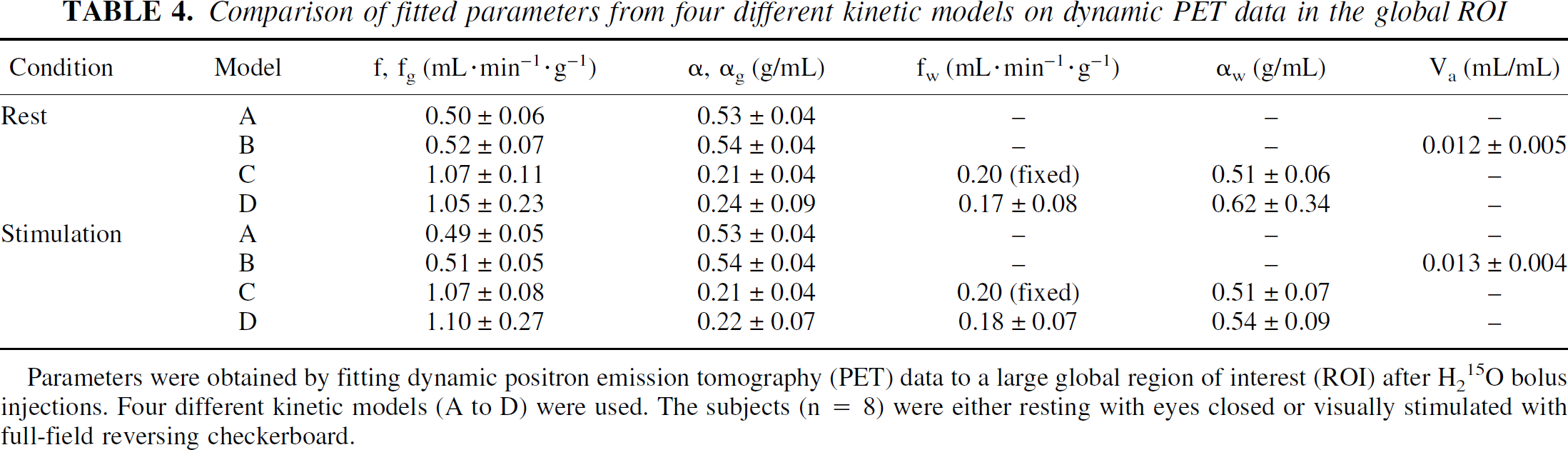
Parameters were obtained by fitting dynamic positron emission tomography (PET) data to a large global region of interest (ROI) after H₂¹⁵O bolus injections. Four different kinetic models (A to D) were used. The subjects (n = 8) were either resting with eyes closed or visually stimulated with full-field reversing checkerboard.

TABLE 5.

Comparison of fitted parameters from four different kinetic models on dynamic PET data in the visual ROI

Condition	Model	f, f_g(mL·min⁻¹·g⁻¹)	α, α_g (g/mL)	f_w(mL·min⁻¹·g⁻¹)	α_W (g/mL)	V_a (mL/mL)
Rest	A	0.55 ± 0.07	0.50 ± 0.09	–	–	–
	B	0.56 ± 0.08	0.50 ± 0.09	–	–	0.009 ± 0.004
	C	0.95 ± 0.13	0.25 ± 0.05	0.20 (fixed)	0.40 ± 0.09	–
	D	1.03 ± 0.29	0.24 ± 0.10	0.18 ± 0.10	0.55 ± 0.38	–
Stimulation	A	0.64 ± 0.07	0.49 ± 0.05	–	–	–
	B	0.68 ± 0.07	0.51 ± 0.04	–	–	0.017 ± 0.005
	C	1.31 ± 0.11	0.27 ± 0.03	0.20 (fixed)	0.39 ± 0.06	–
	D	1.40 ± 0.26	0.26 ± 0.08	0.20 ± 0.10	0.54 ± 0.31	–

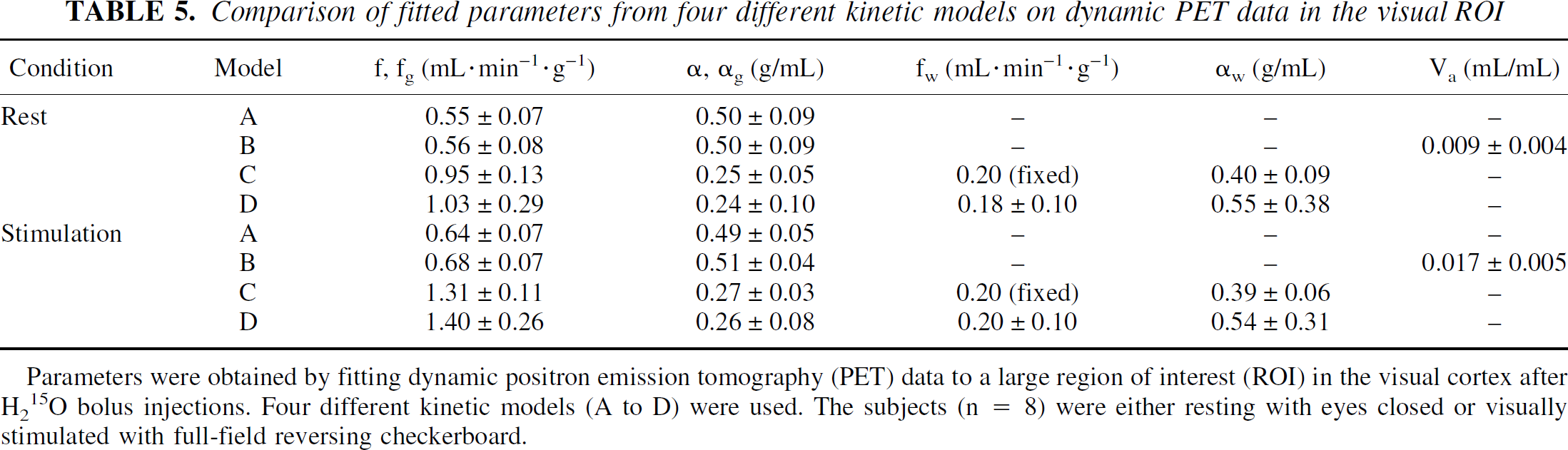
Parameters were obtained by fitting dynamic positron emission tomography (PET) data to a large region of interest (ROI) in the visual cortex after H₂¹⁵O bolus injections. Four different kinetic models (A to D) were used. The subjects (n = 8) were either resting with eyes closed or visually stimulated with full-field reversing checkerboard.

In the global ROI, the f and f_g values did not change significantly with visual activation, although as expected, this was true for the visual ROI. Also in this ROI a significant model × state interaction (P < 0.001) was found indicating a model dependent change in the activation response in absolute values. As shown in Table 5, the activation responses in absolute values are larger in Model C and D than in Model A and B. The significant main effect of state was also present using Model C alone.

The average f_w value in the global ROI (D, 0.18 mL·min⁻¹·g⁻¹, 0.07 SD) was significantly smaller (P < 0.01) than the fixed value of 0.2 mL·min⁻¹·g⁻¹ (Model C), but no changes were found by visual stimulation, acquisition, or repeat.

The average white matter PTFs, α_w, in the visual ROIs, but not in the global ROI, were significantly larger (P < 0.01) in Model D (0.54 g/mL, 0.35 SD) compared with Model C (0.40 g/mL, 0.06 SD, Fig. 4). Also, α_w was unaffected by visual stimulation, acquisition, or repeat.

A significant effect of visual stimulation was found in the visual ROI (P < 0.001) for the ARG model and a significant effect of acquisition mode (3D > 2D; P < 0.001; Table 6) in the white matter ROI.

TABLE 6.

Comparison of the autoradiographic regional cerebral blood flow data (ARG rCBF)

Condition	Acquisition	Global ROI(mL·min⁻¹·g⁻¹)	Visual ROI(mL·min⁻¹·g⁻¹)	White matterROI (mL·min⁻¹·g⁻¹)
Rest	2D	0.43 ± 0.04	0.43 ± 0.05	0.17 ± 0.02
	3D	0.43 ± 0.03	0.42 ± 0.04	0.21 ± 0.01
Stimulation	2D	0.42 ± 0.04	0.54 ± 0.05	0.17 ± 0.02
	3D	0.42 ± 0.04	0.54 ± 0.06	0.21 ± 0.02

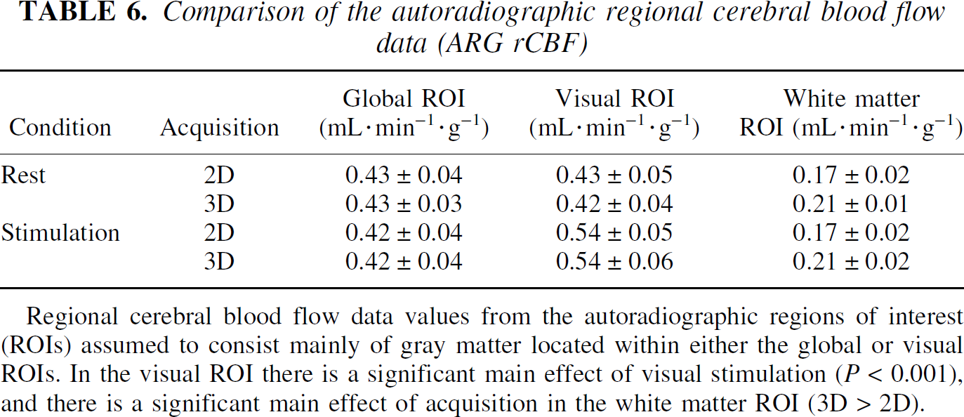
Regional cerebral blood flow data values from the autoradiographic regions of interest (ROIs) assumed to consist mainly of gray matter located within either the global or visual ROIs. In the visual ROI there is a significant main effect of visual stimulation (P < 0.001), and there is a significant main effect of acquisition in the white matter ROI (3D > 2D).

Estimated tissue volumes

The number of voxels selected was 7,501 (2,604 SD) for the visual ROI and 40,074 (4,700 SD) for the global ROI. In Model C, f_g converted to average gray matter global and visual ROI volumes of 143 mL (22 SD) and 33 mL (10 SD), respectively, and the corresponding values for white matter volumes for the two regions were 347 mL (70 SD) and 49 mL (15 SD; Table 7).

TABLE 7.

Average gray matter flow and tissue volumes with corresponding coefficients of variance using model C

	Gray matter flow (f_g)		Gray matter volume		White matter volume

ROI	Mean (mL·min⁻¹·g⁻¹)	CV (%)	Mean (mL)	CV (%)	Mean (mL)	CV (%)
Global	1.07 ± 0.11	6.4 ± 1.9	143.2 ± 22.4	12.7 ± 5.1	346.9 ± 70.4	7.0 ± 1.4
Visual			32.9 ± 10.4	14.1 ± 7.2	48.9 ± 15.1	12.5 ± 10.1
Rest	0.95 ± 0.13	8.3 ± 4.6
Stimulation	1.31 ± 0.11	4.3 ± 2.2

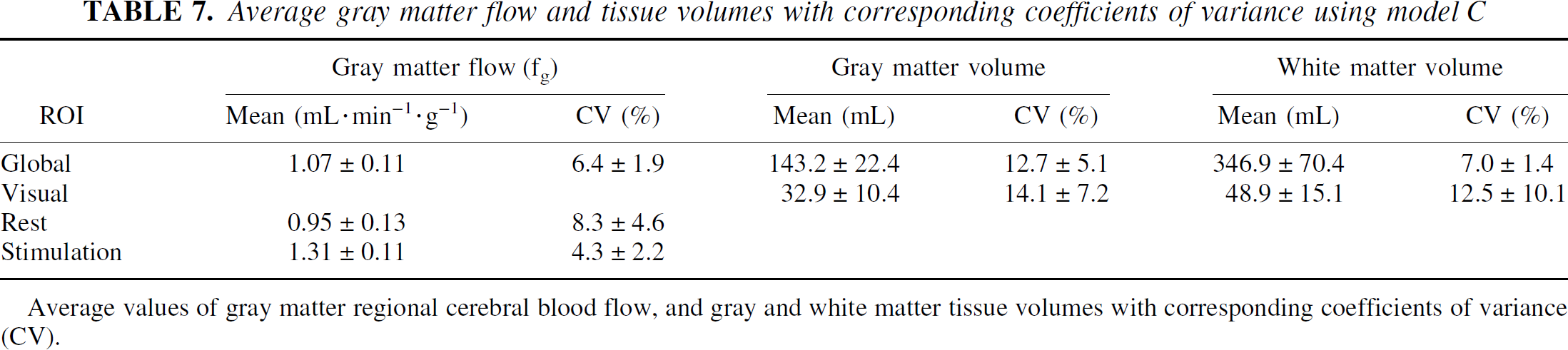
Average values of gray matter regional cerebral blood flow, and gray and white matter tissue volumes with corresponding coefficients of variance (CV).

Reproducibility

The average intrasubject CV for the gray matter flow during rest was 6% for a large ROI, whereas the corresponding value for the ARG rCBF values was 8%. The average intrasubject CV for the calculated gray and white matter tissue volumes were 13% and 7%, respectively (Table 7).

The average CVs for the 300 voxel ROIs were approximately 20% to 35% for the fitted parameters (α_g, f_g, and α_w) and 12% to 17% for the calculated products (α_g * f_g and α_g * f_g + α_w * 0.2 mL·min⁻¹·g⁻¹, respectively). Increasing ROI size to 1200 voxels reduced the average CVs to half of these values (Fig. 6).

FIG. 6.

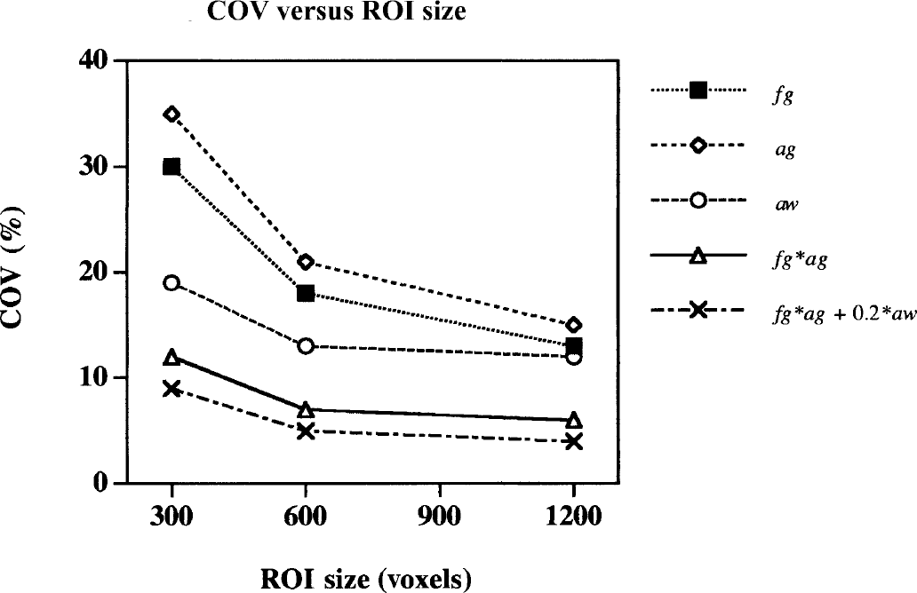
Reproducibility measured as the coefficient of variance (CV) as a function of region of interest (ROI) size. The Model C fitted parameters (α_g, f_g, and α_w) and calculated parameter products (αg * f_g, and α _g * f_g + α_w * 0.2 mL·min⁻¹·g⁻¹) are shown.

Activation response

The Friedman test across quantification models rejected the null-hypothesis of equal percent activation response for the quantitative data (P < 0.0005; χ² = 22.1; df = 4) and after normalization (P < 0.001; χ² = 18.5; df = 4). The post hoc Wilcoxon paired signed rank tests of the activation response can be summarized for both the quantitative and normalized data as the logical expression: Model A = Model B < ARG < Model C. Because of the large variance of the activation responses, Model D was not significantly different from the other models (Fig. 7).

FIG. 7.

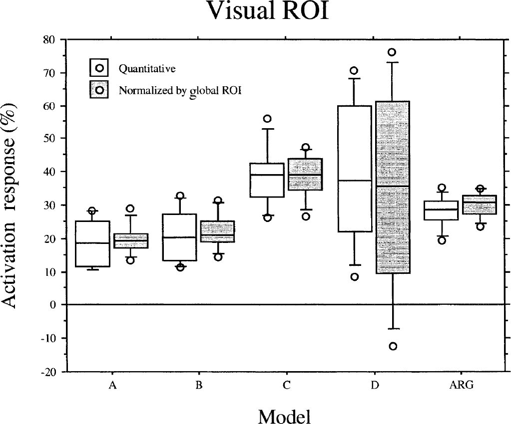
Box plot of the activation response in the visual region of interest (ROI) in percent of the baseline values across five different models. The five horizontal lines of each box show the 10th, 25th, 50th (median), 75th, and 90th percentile of the activation response. Outliers outside the limits are plotted separately. Median activation response using Model C (39.1%) is significantly greater compared with Model A (18.6%), Model B (20.3%), and the autoradiographic model (27.3%), but can not be distinguished from Model D (37.4%).

DISCUSSION

Model stability and estimated parameters

In the current study we report data obtained from four different kinetic models for estimating rCBF after injection of the diffusible tracer, H₂¹⁵O. Two of the models (C and D) included parameter estimations of the PTF (α_w) in a slow flow compartment, which primarily consisted of white matter tissue, whereas the perfusion rate (f_w) in this compartment was either fixed (C) or estimated (D). The slow flow compartment was not included in the two other models (A and B). This means that the flow and PTF estimated using Models A and B represents a weighted average of fast and slow flow tissues. Because of the faster tracer washout from the gray matter, the later PET images of a dynamically sampled sequence will be increasingly influenced by counts from the white matter compartment. This explains the gradually decreasing rCBF values (Fig. 2) and increasing PTF values (Fig. 3) with the length of the fitting period with Models A and B. The estimated parameters using these models are consequently unstable in the sense that the values depend on the length of the fitting period. Notably, the f values (A and B) at a fitting period of 1 minute are still below the values obtained for the f_g values (C) fitting for 6 minutes, which must be caused by a significant contribution of white matter counts in the early images as well.

Model C was the only model that had convincingly stable values as a function of fit time. The average values stabilized after a fitting period of 3 minutes, but a reduction of the CV could still be gained by prolonging the fit to 6 minutes. At this length of fit Model C proved the most optimal based on the AIC, which corresponds to the conclusion reached in our previously reported monkey study (Iida et al., 2000). We do not know if increasing the acquisition period even further would bring about additional CV improvements. After 6 minutes the tracer content in the brain was below 10% of the peak value because of decay and washout, therefore, the benefit of additional data points might be very small.

It should be noted, however, that the cost of the low CV in Model C is the assumption of a white matter rCBF of 0.20 mL·min⁻¹·g⁻¹. This may be a weakness in a clinical setting in which white matter pathology may be present. Actually, the average global ROI f_w value of 0.18 mL·min⁻¹·g⁻¹ (Table 4) using Model D differed significantly from this assumed value. The slightly lower value is likely to reflect inclusion of slowly perfused extracerebral tissues, that, according to previous studies, have a flow of approximately 0.05 mL·g⁻¹·min⁻¹ (Friberg et al., 1986). Model C also gave the largest average activation response (Fig. 7).

The overall worst performance in terms of intersubject variability of the fitted parameters came from Model D. A contributing factor to this could be an extreme sensitivity to errors of delay and dispersion of the input curve as have been shown by simulation studies (Iida et al., 2000).

The doubling of α_g CV (C) compared with α CV (A and B; Fig. 3) reflects a decrease in α_g with an equal standard deviation of 0.04 g/mL. Part of this variability is model invariant as the α, α_g measure represents a spatial fraction influenced by intersubject differences in ROI identification. Thus, it does not necessarily reflect poor model stability.

The importance of the inclusion of V_a in rCBF quantification models has been stressed previously (Fujita et al., 1997; Ohta et al., 1996). However, in our comparison, Model B performed the worst based on the AICs (Table 2, Fig. 5). Although we did find a V_a value significantly different from zero, the value was rather small. The data was to a larger extent dominated by the existence of two compartments, consequently we can not endorse Model B.

Obtained values for gray matter blood flow of approximately 1.00 mL·min⁻¹·g⁻¹ are somewhat higher that what have been found previously with the Xenon clearance techniques (Høedt-Rasmussen, 1965,1967; Høedt-Rasmussen et al., 1966), which would give values of approximately 0.80 mL·min⁻¹·g⁻¹. Contributing to this could be errors in the assumption of the brain tissue-to-blood partition coefficient value for water. An error in the gray matter partition coefficient of 10% (p_g), for example, relates proportionally to an error in the gray matter blood flow (f_g) (10% parameter overestimation), and inversely proportional to an error in the gray matter PTF (α _g ; 10% parameter underestimation) (Iida et al., 2000).

Partial volume correction of cerebral blood flow

Estimated f_g values from Model C and D were significantly increased compared with f values (100%) from Models A and B, and the ARG rCBF values (150%). A similar relation between models was found in the previous monkey study (Iida et al., 1999), thus confirming our a priori expectations.

Partial volume effect correcting techniques based on registration to structural imaging modalities (Herscovitch et al., 1986; Meltzer et al., 1996; Muller-Gartner et al., 1992; Rousset et al., 1998; Schlageter et al., 1987; Videen et al., 1988) have been concerned primarily with correcting separately measured values of the regional glucose metabolism. Average regional increases after PVE correction in the cortical gray matter of healthy controls have been reported as varying from 10% to 50% (Labbe et al., 1996) depending on scanner resolution, reconstruction filtering, and cerebral region. The largest disadvantage of this approach is the practical requirements of structural images with the added cost for image acquisition and data processing. Using magnetic resonance imaging will require correction of magnetic field inhomogeneities, which, however, will not correct the changes in gray—white matter contrast in the MR images. This together with the MR image PVE and PET-MRI misregistration errors can lead to missegmentation. Furthermore, a validation of the tissue categories derived from the various segmentation techniques against histologic criteria, or physiologic criteria, or both, is often missing. Conversely the kinetic modeling approach based on physiology alone can cost-effectively estimate tissue volumes and PVE corrected rCBF values simultaneously without reference to structural imaging techniques. This would be of particular interest in the study of patients with particular thin gray matter (for example, in children) or cerebral pathology characterized by atrophy (for example, Alzheimer's disease), in which the regional gray matter flow values will be falsely underestimated using the ARG method alone.

It should be noted that as the model essentially fits a fast and a slow flow component there is a possibility that the value in an isolated area of gray matter would be low enough to be modeled as white matter. This would underestimate gray matter PTF and overestimate gray matter rCBF, whereas white matter PTF and white matter rCBF would be overestimated. However, if the white matter flow is also reduced, preserving the gray—white matter contrast, errors may not arise. Further investigation is needed.

Reproducibility

The average intrasubject CV of f_g was 6% to 8% during rest, which is in the same range as the ARG rCBF values in the same regions (Table 7). The average intrasubject CV of the calculated gray matter tissue volumes was approximately 14%. There are several error sources that could potentially contribute to this value. One obvious error source is within modality misregistration (PET-to-PET), the size of which depends on the ROI configuration and the nature of movement. Validation studies using a 3D brain phantom show that the AIR algorithm aligns PET images with maximum positional errors that are usually less than the width of a voxel (Woods et al., 1992); thus a positional error in the order of 1 to 2 mm could be expected. To estimate the effect of a 1-mm parallel translation in the z-direction of the global ROI, the ratio of the number of voxels in the bottom ROI slice times 1/4.25 to the total number of global ROI voxels was calculated for all subjects. The average impact of a movement of this kind was a change in the global ROI volume of 3.4% per millimeter (SD 0.3). This error would translate directly into the estimated gray matter volume providing that the PTF of the tissue was approximately equal to the average for the whole ROI, and that the movement was not compensated in the other end of the ROI by an exclusion of tissue. This latter point was unlikely with our ROIs that were placed well outside the cortex.

Simulation studies show that a 2-second error of the delay or dispersion can lead to a 2% error in the estimation of the PTF. Furthermore, should the true average white matter flow in the ROI deviate 0.01 mL·min⁻¹·g⁻¹ from the assumed value of 0.20 mL·min⁻¹·g⁻¹ this would translate into an error of approximately 3% (Iida et al., 2000).

The CV for fitted parameters using small ROIs of 300 voxels was rather large (20% to 35%), whereas the larger ROI sizes of 600 and 1200 voxels gave acceptable values of approximately 15% (Fig. 6). It should be noted that correction of possible confounding global differences was not performed. The CVs for the calculated products (α * f_g and α_g * f_g + α_w * 0.2 mL·min⁻¹·g⁻¹) followed the same pattern of reduction with increasing ROI size, but were only half of the values of the fitted parameters.

Fitting the parameters on a voxel-by-voxel basis was thus not a realistic strategy for this model. However, as outlined in the current study, the placement of ROIs around larger continuous clusters of reduced or increased rCBF could be guided by an initial SPM type analysis of ARG rCBF images. A post hoc dynamic fitting procedure would allow for a more differentiated analysis of the parameters under investigation applied not only to normal physiology, but also to pathologic conditions. Thus, for activation studies, in which physiology rather than localization is of interest, or clinical group analyses of, for example, patients versus normal controls, the presented techniques provide a supplement, rather than a substitute, for the existing simpler ARG PET technique.

2D versus 3D acquisition

Statistically there were no differences between 2D and 3D acquisition, either as main effects or interactions, in any of the fitted parameters. Only with respect to the ARG rCBF in the white matter region was there a significant increase (Table 6). Contributing to this were several factors including decreases in axial resolution during 3D acquisition caused by the removal of septa covering part of the crystals (Lewellen et al., 1996), the use of 2D transmission scans in the reconstruction of 3D data, and differences in scatter correction methods. Thus, with this limitation in mind for future quantitative rCBF studies using dynamic or ARG models with the GE-Advance PET scanner, it is recommended that they all be performed in 3D acquisition mode. In application of the method the injected dose, which was limited in the current study because of a combination of ethical considerations and design, could easily be increased from 200 MBq to 600 MBq. This would give a considerable advantage in the signal-to-noise characteristics of the PET images (Holm et al., 1996), the arterial input curves, and possibly the resulting model fits and image alignment procedure. The measured reproducibility measures for the small ROI could thus be improved even further.

Activation response

The model including the contribution of a fixed slow tissue flow component (C) gave a significant increase in the activation response over models that did not include the contribution(A and B, Fig. 7). In Model C we found that the slow tissue flow component on average consisted of two-thirds of the visual ROI tissue voxels (Table 5), which is likely derived from extracerebral regions. During stimulation the f_w increased from 0.18 mL·min⁻¹·g⁻¹ to 0.20 mL·min⁻¹·g⁻¹ using Model D, which was not significant. The power of this analysis, however, is rather weak because of the high CV of the measure. The ARG rCBF activation response was the intermediary between Models A and B and Model C. It should be noted that as the visual ROIs were defined based on the ARG rCBF images the results could be biased towards this model. Normalization to the global ROI affected mainly the variation of the activation response, which was reduced with the exception of Model D (Fig. 7). The instability of this model can be credited for this effect, thus the model noise contribution had a greater influence than global rCBF changes on the variability in the visual ROI values. This increased Model D variation can also explain that the χ² value is lower in the normalized compared with the quantitative data.

In conclusion, the current study clearly demonstrates the importance of PVE correction in the quantitation of rCBF in normal humans. In a region assumed to consist primarily of gray matter the PVE contributes to the underestimation of the absolute ARG CBF value by 50%, and more interestingly, to the underestimation of the gray matter CBF response to visual stimulation.

Footnotes

Acknowledgments

The authors acknowledge Karin Stahr and the staff at the PET center at Rigshospitalet, Copenhagen, for their participation. Furthermore, the John and Birthe Meyer Foundation is gratefully acknowledged for donating the Cyclotron and PET scanner.

Abbreviations used

References

Akaike

(1974) A new look at the statistical model identification. IEEE Transaction on Automatic Control AC-19:716–723

Belliveau

Kennedy

McKinstry

Buchbinder

Weisskoff

Cohen

Vevea

Brady

Rosen

(1991) Functional mapping of the human visual cortex by magnetic resonance imaging. Science 254:716–719

DeGrado

Turkington

Williams

Stearns

Hoffman

Coleman

(1994) Performance characteristics of a whole-body PET scanner. J Nucl Med 35:1398–1406

Fox

Raichle

(1984) Stimulus rate dependence of regional cerebral blood flow in human striate cortex, demonstrated by positron emission tomography. J Neurophysiol 51:1109–1120

Fox

Raichle

(1985) Stimulus rate determines regional brain blood flow in striate cortex. Ann Neurol 17:303–305

Frackowiak

Friston

(1994) Functional neuroanatomy of the human brain: positron emission tomography—a new neuroanatomical technique. J Anat 184:211–225

Friberg

Kastrup

Hansen

Bulow

(1986) Cerebral effects of scalp cooling and extracerebral contribution to calculated blood flow values using the intravenous 133Xe technique. Scand J Clin Lab Invest 46:375–379

Fujita

Meyer

Reutens

Kuwabara

Evans

Gjedde

(1997) Cerebral [(15)O] water clearance in humans determined by positron emission tomography: II. Vascular responses to vibrotactile stimulation. J Cereb Blood Flow Metab 17:73–79

Herscovitch

Auchus

Gado

Chi

Raichle

(1986) Correction of positron emission tomography data for cerebral atrophy. J Cereb Blood Flow Metab 6:120–124

10.

Herscovitch

Raichle

(1985) What is the correct value for the brain—blood partition coefficient for water? J Cereb Blood Flow Metab 5:65–69

11.

Holm

Law

Paulson

(1996) 3D PET activation studies with an H215O bolus injection. In: Quantification of brain function using PET ( Myers

R CV

Bailey

Jones

, eds), San Diego, CA:Academic Press, pp 93–97

12.

Høedt-Rasmussen

(1965) Regional cerebral flow in man measured externally following intra- arterial administration of 85-Kr or 133-Xe dissolved in saline. Acta Neurol Scand Suppl 14:65–68

13.

Høedt-Rasmussen

(1967) Regional cerebral blood flow. The intraarterial injection method. Copenhagen, Denmark: University of Copenhagen

14.

Høedt-Rasmussen

Sveinsdottir

Lassen

(1966) Regional cerebral blood flow in man determined by intra-arterial injection of radioactive inert gas. Circ Res 18:237–247

15.

Iida

Higano

Tomura

Shishido

Kanno

Miura

Murakami

Takahashi

Sasaki

Uemura

(1988a) Evaluation of regional differences of tracer appearance time in cerebral tissues using water and dynamic positron emission tomography. J Cereb Blood Flow Metab 8:285–288

16.

Iida

Kanno

Miura

Murakami

Takahashi

Uemura

(1986) Error analysis of a quantitative cerebral blood flow measurement using H2(15)O autoradiography and positron emission tomography, with respect to the dispersion of the input function. J Cereb Blood Flow Metab 6:536–545

17.

Iida

Kanno

Takahashi

Miura

Murakami

Takahashi

Ono

Shishido

Inugami

Tomura

(1988b) Measurement of absolute myocardial blood flow with H215O and dynamic positron-emission tomography. Strategy for quantification in relation to the partial-volume effect. Circulation 78:104–115

18.

Iida

Law

Pakkenberg

Hansen

Eberl

Holm

Hansen

Thomsen

Svarer

Ring

Friberg

Paulson

(2000) Quantitation of regional cerebral blood flow corrected for partial volume effect using O-15 water and PET: I. Theory, error analysis, and histostereological analysis. J Cereb Blood Flow Metab 20:1237–1251

19.

Iida

Rhodes

de-Silva

Yamamoto

Araujo

Maseri

Jones

(1991) Myocardial tissue fraction-correction for partial volume effects and measure of tissue viability. J Nucl Med 32:2169–2175

20.

Iida

Takahashi

Tamura

Ono

Lammertsma

(1995) Myocardial blood flow: comparison of oxygen-15-water bolus injection, slow infusion and oxygen-15-carbon dioxide slow inhalation. J Nucl Med 36:78–85

21.

Kanno

Iida

Miura

Murakami

Takahashi

Sasaki

Inugami

Shishido

Uemura

(1987) A system for cerebral blood flow measurement using an H215O autoradiographic method and positron emission tomography. J Cereb Blood Flow Metab 7:143–153

22.

Labbe

Froment

Kennedy

Ashburner

Cinotti

(1996) Positron emission tomography metabolic data corrected for corticl atrophy using magnetic resonance imaging. Alzheimer Dis Assoc Disord 10:141–170

23.

Lewellen

Kohlmyer

Miyaoka

Kaplan

Stearns

Schubert

(1996) Investigation of the performance of the general electric ADVANCE positron emission tomograph in 3D mode. IEEE Transactions on Nuclear Science 43:2199–2206

24.

Meltzer

Zubieta

Links

Brakeman

Stumpf

Frost

(1996) MR-based correction of brain PET measurements for heterogeneous gray matter radioactivity distribution. J Cereb Blood Flow Metab 16:650–658

25.

Muller-Gartner

Links

Prince

Bryan

McVeigh

Leal

Davatzikos

Frost

(1992) Measurement of radiotracer concentration in brain gray matter using positron emission tomography: MRI-based correction for partial volume effects. J Cereb Blood Flow Metab 12:571–583

26.

Ohta

Meyer

Fujita

Reutens

Evans

Gjedde

(1996) Cerebral [(15)O]water clearance in humans determined by PET: I. Theory and normal values. J Cereb Blood Flow Metab 16:765–780

27.

Raichle

Martin

Herscovitch

Mintun

Markham

(1983) Brain blood flow measured with intravenous H2(15)O. II. Implementation and validation. J Nucl Med 24:790–798

28.

Rousset

Evans

(1998) Correction for partial volume effects in PET: principle and validation. J Nucl Med 39:904–911

29.

Schlageter

Horwitz

Creasey

Carson

Duara

Berg

Rapoport

(1987) Relation of measured brain glucose utilisation and cerebral atrophy in man. J Neurol Neurosurg Psychiatry 50:779–785

30.

Smith

Tong

Lammertsma

Butler

Schnorr

Watson

Ramsay

Clark

Jones

(1994) Dosimetry of intravenously administered oxygen-15 labeled water in man: a model based on experimental human data from 21 subjects. Eur J Nucl Med 21:1126–1134

31.

Stearns

(1995) Scatter correction method for 3D PET using 2D fitted gaussian functions. J Nucl Med 36:105P

32.

Vafaee

Meyer

Marrett

Paus

Evans

Gjedde

(1999) Frequency-dependent changes in cerebral metabolic rate of oxygen during activation of human visual cortex. J Cereb Blood Flow Metab 19:272–277

33.

Videen

Perlmutter

Mintun

Raichle

(1988) Regional correction of positron emission tomography data for the effects of cerebral atrophy. J Cereb Blood Flow Metab 8:662–670

34.

Woods

Cherry

Mazziotta

(1992) Rapid automated algorithm for aligning and reslicing PET images. J Comput Assist Tomogr 16:620–633

Quantitation of Regional Cerebral Blood Flow Corrected for Partial Volume Effect Using O-15 Water and PET: II. Normal Values and Gray Matter Blood Flow Response to Visual Activation

Abstract

Keywords

METHODS

Subjects

Experimental design

PET scanning

MRI scanning

Image processing and regions of interest

Fitting procedure

Calculations and statistical evaluation

Model stability

Optimal model

Statistical evaluation

Estimated tissue volumes

Reproducibility

Activation response

RESULTS

Physiologic data

Model stability

Optimal model

Effects of acquisition, behavioral state, and repeat on the model parameters

Estimated tissue volumes

Reproducibility

Activation response

DISCUSSION

Model stability and estimated parameters

Partial volume correction of cerebral blood flow

Reproducibility

2D versus 3D acquisition

Activation response

Footnotes

Acknowledgments

Abbreviations used

References