Responding to new information in a mining complex: fast mechanisms using machine learning

Abstract

As more and more data about mining complex operations are collected and stored, it becomes increasingly important for computer systems to help human operators make better, more informed decisions. This can be done indirectly, through improved visualization or prediction, or directly by suggesting decisions that respond to new information. This paper contributes to the direct approach by showing how state-of-the-art data-driven decision making can be used for optimizing material flows in a large mining complex. To this end, a combination of neural networks and policy gradient reinforcement learning is used for computing material destination decisions that automatically respond to new information. Results using a computational model of a large copper mining complex show that the proposed method significantly outperforms an optimized cut-off grade policy similar to the one currently used at the mine.

Introduction

Due to decreased sensor and storage cost and increase standardization and ease of use, more and more data are collected about the operation of industrial processes. In mining, in particular, information concerning the properties of material as it flows through the mining complex can be collected using near-infrared reflectance spectroscopy (Goetz et al. 2009) or camera images (Chatterjee 2013; Horrocks et al. 2015) in addition to the more traditional blasthole and in-fill drilling analysis. Material can also be better located thanks to the use of GPS devices on hauling equipment or RFID tags embedded in the material (La Rosa et al. 2007). Benndorf and Jansen (2017) provide an overview of the state of these data collection methods in the industry, as well as surveying existing and proposed closed-loop optimization methods that can leverage it.

All this data can assist better understand the functioning of the mining complex and assist in making decisions that adapt to the new situations encountered. For instance, if too much material is waiting at one of the crushers in a multi-crusher complex, then staff might decide to re-route some of the material bound for that crusher to others that are less busy. However, as the amount of available data collected increases, it becomes more and more difficult to ensure that the best decisions are being made in light of the new information.

This paper attempts to alleviate these issues by introducing a new system for automatically selecting the best way to respond to new information. The system is based on data-driven stochastic optimization techniques originating in the field of reinforcement learning (Sutton and Barto 1998). In the last few years, reinforcement learning has seen notable successes in simulated domains, such as producing the first Go algorithm to successfully compete against the best human players (Silver et al. 2016) or playing video games based on pixel information alone (Mnih et al. 2015). These successes have inspired companies to include it as a core part of their operation, such as Microsoft's Multiworld Testing framework 1 or Google's adaptive data center cooling. 2 An important advantage of reinforcement learning methods over other optimization techniques is that the decision-making policies they compute explicitly encode what decisions to make in different situations. By contrast, decisions computed using more traditional optimization approaches, such as mixed integer stochastic programming, have to be re-optimized every time the system's state changes as a result of new information. This can make them too slow for practical use when decisions need to be frequently updated. More subtly, the complexity of evaluating the effect of a re-optimization strategy can scale exponentially if the decisions made before time affect the optimality of decisions made after time .

The standard stochastic programming response to these concerns is multi-stage stochastic programming (MSP) (Birge and Louveaux 1997; Boland et al. 2008; Del Castillo and Dimitrakopoulos 2018). Given a set of realizations of uncertainty, typically referred to as scenarios, MSP computes scenario-dependent decisions whose inherently optimistic nature is kept in check through the use of non-anticipativity constraints. By modelling how decisions should respond to different scenarios, MSP can approximately evaluate the effect of re-optimizing decisions in light of new information. However, computing the optimal decision for measurement values not present in the scenarios using MSP is heavily dependent on the metric used to measure how similar different scenarios are, and it is rarely clear how to specify such a metric. By contrast, reinforcement learning can leverage modern machine learning methods in order to automatically infer the similarity between different situations. The relationship between MSP and reinforcement learning has been analyzed by various researchers (Defourny et al. 2012; Powell 2012; Powell et al. 2012).

The use of reinforcement learning for mining complex optimization has already been explored by Paduraru and Dimitrakopoulos (2014). However, their work has the drawback that the decisions made for each block depend explicitly on the position that the respective block has in a fixed extraction sequence. This limits the use of their method to settings where the extraction sequence is fixed and pre-defined, ignoring the reality that the order in which the material is extracted is rarely known in advance, especially for multi-pit mining complexes. The main contribution of this paper is to propose an alternative reinforcement learning approach that overcomes these limitations and to showcase its application using a challenging mining complex optimization problem. The first part is accomplished by using more powerful reinforcement learning methods that leverage the capabilities of modern neural networks. The second part involves building a stochastic hour-by-hour model of material flow based on geostatistical simulations and equipment performance data for a large multi-pit copper mining complex. The model is used for generating training data for the reinforcement learning approach and for comparing the proposed method to an optimized cut-off grade policy modelled based on the current practice at the mine.

The remainder of the paper proceeds as follows. Section ‘Stochastic operational modelling of a mining complex’ describes the rationale and implementation for the stochastic hour-by-hour material flow model. Section 3 describes a method for optimizing material flow by using neural network based reinforcement learning and shows how this method can be applied to the model introduced in Section ‘Stochastic operational modelling of a mining complex’. The resulting implementation is then compared to an optimized cut-off grade policy, and the results are presented in Section ‘Case study’. Finally, conclusions and future work are discussed in Section ‘Conclusions’.

Stochastic operational modelling of a mining complex

Material extracted in a mining complex undergoes various transformations before the concentrated or refined product is shipped to customers. Understanding the effect of these transformations, as well as the associated cash flows, can help develop better planning strategies and provide a more realistic assessment of their impact. Therefore, this section focuses on developing realistic models of material flow in a mining complex, starting by discussing general concepts and then describing a particular implementation for a multi-pit copper mining complex.

Material flows, which determine the revenues obtained from the final product and the operating costs, depend on several factors, including geology, transportation availability, and processing characteristics. Since none of these factors can be known a priori with full precision, explicitly modelling the uncertainty is necessary for identifying and managing risk. This work uses the common approach of incorporating geological uncertainty via a set of geostatistical simulations. A wide range of models that can produce a set of simulations capturing geological uncertainty have been proposed over the years (Goovaerts 1997; Strebelle 2002; Zhang et al. 2006; Remi et al. 2011; Boucher and Dimitrakopoulos 2012; Soares et al. 2017; Minniakhmetov et al. 2018). These can be combined with a stochastic model of extraction, transportation, and processing, producing a set of joint simulations that reflect the combined uncertainty. For the purpose of this paper, extraction and transportation uncertainty refers to the time it takes to extract material and transport it between various points in the mining complex. There are several potential sources for this temporal uncertainty, including:

equipment breakdown and repair times

truck and shovel cycle times

queuing times for trucks, either at the origin (shovel) or at the destination (crushers, plants, leach pads etc.)

The uncertainty in crushing and processing times is partly due to geometalurgical properties, such as SPI (Sag Power Index), BWI (Bond Work Index) and many other material property attributes (Sepúlveda et al. 2018). It can also be due to equipment breakdown or additive (un)availability.

The different transformations undergone by extracted material can add non-temporal uncertainty to the material flows. For instance, the level of coarseness resulting from crushing, recovery rates at the plants or leach pads, or amount of deleterious elements in concentrate may all exhibit variability. Part of this variability can be explained by quantities that can be measured; for instance, it is common for recovery to be affected by head grade. However, there may also be unmeasured or imperfectly measured quantities that cause variability in the output of transformations. Therefore, this paper proposes a mixed approach: the outcome of transformations is modelled using a sum of a regression output and stochastic noise, with the regression covariates being the quantities that are known to affect the output of interest. An example of this is illustrated in Section ‘System dynamics’.

The sources of uncertainty described above make it clear that there can be multiple interactions that determine the amount of time a certain activity takes. Some of these interactions include:

Crushing and processing times depend on the rate of material sent to crushers and plants, which in turn depends on cycle times and extraction rates.

Queuing times are affected by

○ the relationship between shovel productivity and the number of trucks assigned to each shovel,

○ the number of trucks sent to the same destination,

○ cycle times and extraction rates,

○ crushing and processing times.

Extraction rates can be affected by queuing times if the shovel has to wait for trucks.

Plant recovery rates can be affected by crushing parameters and performance.

These interactions can be modeled using various methodologies, such as discrete event simulation (Zeigler et al. 2000), system dynamics (Sterman 2000), or agent-based modelling (Railsback and Grimm 2012). For a survey of the use of these methodologies in mining, see Raj et al. (2009). More recently, discrete event simulation has been used for modelling truck-shovel systems by Jaoua et al. (2012). The model proposed in this paper combines discrete event simulation and system dynamics concepts, and will be outlined in the following section.

Case study implementation

A diagram of the material flow for the copper mining complex used in the case study is shown in Figure 1. There are two pits, and five shovels for each pit. Material extracted by each of the shovels is transported by truck to one of the four crushers (C1, C2, C3 and C5) or to one of the two leach pads. Each pit can only send materials to a subset of the crushers, as indicated by the arrows in Figure 1. Crushed material is sent on conveyor belts to one of the three plants, with the plants that each crusher can send material to also indicated by arrows in Figure 1. The final product is either copper concentrate (from the plants) or copper cathodes (from the leach pads). The details of the stochastic model built for this case study are presented in the following sections.

Figure 1

Material flow diagram for the mining complex considered. Images are available in colour online.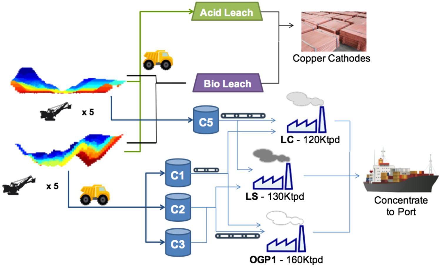

Material representation

The material flowing through the mining complex is represented using a set of additive properties, similarly to Goodfellow and Dimitrakopoulos (2016, 2017). For this case study, the properties are tonnage, copper content, amount of soluble copper, and arsenic (in ppm). When material from different sources is combined, some of these properties are added (e.g. tonnage, copper content) and others are computed as a mass-weighted average (e.g. arsenic concentrations). The various destinations in the mining complex can effect non-linear transformations on the material. For this case study, hardness-related properties are not considered; therefore, the transformations performed by the crushers are not considered.

Discrete event simulation

Because destination decisions for the material being sent from the shovels to the crushers are made at the block level, and blocks are clearly defined discrete units, discrete event simulation is used for modelling material flow up to the crushers. More precisely, a discrete event is triggered whenever:

The shovel finishes extracting a block (and starts extracting the next); this is determined by the amount of time it takes to extract the current block, which is encoded by a variable .

The block first reaches the crusher, which is modelled by a variable called .

To compute , the following assumptions are made:

Under perfect transportation and mechanical availability (meaning that a truck is always ready to be loaded and the shovel does not break down), extraction time is assumed, for reasons of simplicity in the present study, to follow a normal distribution. The mean and standard deviation of this distribution were generated from historical data.

The shovel can break down according to an exponentially distributed failure model. If the shovel does break down, the time it takes to get it back online is assumed to have a log-normal distribution (because the repair time must be greater than zero). Since no data regarding shovel breakdowns was available, the parameters of these two distributions were assigned arbitrary values; the expected value of the resulting random variables were 600 h for the time to failure and 12 h for the repair time. Adding shovel breakdown times to the ideal-conditions extraction time results in a random variable called .

Extraction times are also impacted by the time that the shovel has to spend waiting for trucks. If the block is being sent to the crusher, the waiting time is determined by the following two quantities:

Truck cycle times, which similarly to shovel times are modelled herein using a normal distribution under perfect mechanical availability. The mean of that distribution is determined by the depth of the block and the distance to the destination. Modelling the effect of truck breakdowns is more complicated than for shovels, since trucks can be replaced, and modelling each individual truck would have been overly detailed. Therefore, truck breakdowns are accounted for by multiplying the normal operation time above by a constant whenever a ‘breakdown event’ occurs; this is assumed to occur for each block with a fixed probability. The corresponding random variable is called .

The time that trucks have to wait before they unload at the crushers, which depends on how long it takes to crush the materials a block. This, in turn, depends on how much material has already been sent to that crusher. The corresponding waiting time is reflected by the variable , which is computed by adding the tonnage of the allocated block to the tonnage of the material waiting to be crushed and dividing by the (deterministic) crusher throughput.

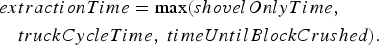
Precisely modelling the effect of transportation and crushing on extraction time requires detailed fleet modelling that is beyond the scope of this work. Instead, the approximation used here accounts for the different bottlenecks by taking the maximum of the three variables defined above, resulting in the random variable being defined as

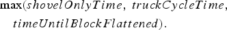
If the block is sent to one of the leach pads, the extraction rate may be constrained by the rate at which material sent to the leach pad can be flattened. This is determined by a variable called , which is the equivalent of above. Consequently, if the block is sent to the leach pad, is considered to be equal to

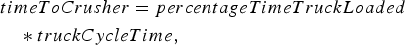
In order to model the time when a block first reaches the crusher, it is assumed that the amount of time that the truck spends loaded (i.e. transporting material from the shovel to the crusher) is a fixed percentage of the cycle time, which is denoted by . Then the time to reach the crusher is simply where is the same value that was used to compute .

System dynamics

System dynamics models typically involve concepts such as stocks, flows, feedback loops and time delays, which are all present for the mining complex considered in this paper. The main difference with respect to discrete event simulation is that system dynamics models tend to divide time into discrete units and compute the total effects of the various interactions within each unit of time, whereas discrete events may be triggered at any point in time and have an immediate event once they are triggered. Because the operation of crushers, plants, conveyor belts and leach pads is marked by very few temporal discontinuities, it was decided to use a system dynamics approach for modelling these parts of the mining complex. Every time step (hour), the following operations occur for the mining complex components modelled using system dynamics:

Each crusher transforms incoming material hauled by trucks into crushed material that gets placed on the conveyor belt connecting it to the destination plant. A list of the blocks processed every hour is maintained and updated each time a block arrives at the crusher or finishes crushing. An equal proportion of each of these blocks is crushed every hour, with the total amount that can be crushed limited by the crusher's (deterministic) throughput. The properties of the crushed material are determined by averaging the properties of the input material.

Crushed material is placed on the conveyor belt corresponding to the destination plant. The conveyor belt determines what fraction of that material will arrive at the plant during each of the subsequent hours.

Each plant uses a feed pile that receives material from the conveyor belts and temporarily stores it before it is processed. The material available for processing during each hour is computed by adding the properties of the material placed on the feed pile during that hour to the properties of the material already on the feed pile. A fraction of that material, computed according to the plant's throughput, is processed each hour. The properties of interest for the concentrate (copper tonnes recovered and arsenic concentration) are the results of transformations whose parameters were estimated using historical data as outlined below.

Determining plant output

The characteristics of the concentrate produced by plants are in general a function of the properties of the input material, additives, processing parameters etc. This function can be fit using historical data, and increasingly complex and accurate models can be used if large amounts of data collected at a high temporal resolution are available. However, only daily production data was available for the case study presented in this paper. Based on this data, the best-performing model for the copper tonnes recovered was simply a linear function of the input grade; similarly, the best-performing model for the amount of arsenic in concentrate was a linear function of the amount of input arsenic concentration. Because significant variability in the output did remain after using these explanatory variables, a stochastic model was used where the variance of the output variable was estimated as a linear function of the input value. For the copper tonnes recovered, this can be written as

The coefficients and were estimated using linear regression based on daily historical data collected during five years of operation. A similar model was used for sampling arsenic concentration.

For the leach pads, only monthly production data was available, resulting in a much smaller data set that made density estimation less reliable. Therefore, the tonnage of recovered copper was estimated as a deterministic linear function of the input grade.

Modelling joint uncertainty

In order to produce a full uncertainty model, the above components need to be merged and combined with a set of available simulations that captures geological uncertainty. The simulated values, including Cu, soluble Cu, and As, are correlated both with each other and spatially. All blocks were assumed to have the same tonnage. The geostatistical simulations are combined with the aforementioned models for material transportation and processing in order to produce a model of the combined uncertainty in the mining complex. This is a generative model, meaning that, rather than providing an analytical form of the joint distribution, it consists of an algorithm for sampling new scenarios from this distribution. For each time horizon , a new scenario is sampled by first randomly selecting one of the geostatistical simulations provided and then subsequently performing the following steps for each time period (hour) :

[1] The material extracted by each shovel is computed by first determining the block(s) extracted during period , and then using the current simulation to determine the properties (Cu, soluble Cu, and As) for the extracted block(s). Each shovel starts period by extracting the same block that was being extracted at the end of period . The time when the block has finished being extracted is computed by sampling and adding it to the time when the block started being extracted. If the resulting value falls within period , a discrete event is triggered, and the shovel moves on to the next block. This next block, as well as the very first extracted block, are determined by a pre-defined extraction order; the optimization of this order is left for future work.

[2] A list containing all the blocks that are being extracted and being sent for crushing is maintained for each of the crushers. Each block has an associated random variable called that encodes the time when the block first reaches the crusher. The value of is computed by adding the time when the block started to be extracted to a sampled value of , which is computed as described in Section ‘Discrete event simulation’.

[3] For each crusher, the blocks being crushed during the period are the blocks that were being crushed at the end of period in addition to the blocks on the list described above for which falls within period . As described in Section ‘System dynamics’, the output of each crusher is placed on the conveyor belt corresponding to the destination plant for period .

[4] The plant feed pile contents during period , as well as the material processed during , are determined based on the conveyer belt material due to reach the plant during that period. The properties of the concentrate produced during period (recovered Cu and As concentration) are then sampled from the stochastic plant model, based on the material processed during .

Computing destination policies

The objective of this work is to compute a policy for determining the initial destination of each block at the time when it starts being extracted. This is done via a reinforcement learning algorithm that uses neural networks. The optimized policy will be compared to a baseline consisting of a cut-off grade policy similar to the one currently in use at the mine. The remainder of this section describes the baseline and optimized policies.

Baseline destination policy

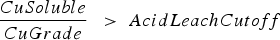
The baseline policy decides where to send each extracted block based on the block's copper grade and soluble copper content. The policy depends explicitly on the ratio between soluble copper and grade – the higher the ratio, the more oxide-like the material is. The cutoff grades for the plants (vs everything else), bio leach (vs waste), and acid leach (vs waste) are denoted by , and , respectively. If the eventual destination is one of the plants, the block is sent to the crusher that has the minimum total tonnage being sent to it at the time when the block needs to be allocated, and the crushed material is placed on the conveyor belt corresponding to the plant with the lowest feed pile tonnage. The baseline policy is summarized below:

If :

If > :

destination =  Min Tonnage Crusher

Else:

If :

 destination = BioLeach

Else:

 destination =  Waste

Else if :

If :

destination = BioLeach

Else:

destination =  Waste

Else:

If :

destination = AcidLeach

Else:

destination =  Waste

Optimized destination policy

This section illustrates how destination policies can be optimized using reinforcement learning. In general, reinforcement learning is concerned with optimizing control policies for time-varying stochastic systems that are, in turn, based on data collected by interacting with the system of interest. For this paper, the system of interest is represented by the stochastic mining complex model outlined in Section ‘Determining plant output’. The class of policies being optimized maintains the same structure as the baseline destination policy but replaces the cutoff-based decisions with optimized sub-policies. The general form of the optimized policy will therefore involve selecting one of three optimized sub-policies, namely, CrusherVsBioLeachVsWastePolicy (that is, the crusher and eventually mill, bio leach and waste dump), BioLeachVsWastePolicy (bio leach and waste dump) and AcidLeachVsWastePolicy (acid leach and waste dump) depending on the value of :

If :

 destination = CrusherVsBioLeachVsWastePolicy

Else if :

 destination = BioLeachVsWastePolicy

Else:

 destination = AcidLeachVsWastePolicy

In reinforcement learning, the policies being optimized are a function of the state of the system being optimized. The state can be informally described as a numerical representation containing all the necessary information about the system of interest. 3 States change over time, reflecting new information obtained about the system. For the case study in this paper, the state is a vector containing the following components, which are updated every time a new block needs to be allocated:

For all sub-policies, the properties (Cu, soluble Cu, and As) of the block being allocated.

For CrusherVsBioLeachVsWastePolicy and BioLeachVsWastePolicy, Cu tonnes and total tonnage of the material placed on the Bio Leach.

For CrusherVsBioLeachVsWastePolicy, Cu tonnes, total tonnage and As of the material already sent to each of the crushers.

For AcidLeachVsWastePolicy, Cu tonnes and total tonnage of the material placed on the Acid Leach.

For all sub-policies, the percentage of the blocks scheduled to be extracted next by every shovel that would get sent to each of the destinations considered by the sub-policy, if they were being allocated using the baseline policy. This provides the neural network with some information about upcoming material.

Policy representation

In reinforcement learning, the term policy has a specific meaning: it is a mathematical function mapping the state space to the decision space. As such, it can be seen as an instantiation of the common use of the word ‘policy’ (‘a course or method of action’). Expressing policies as explicit functions of the state allows them to be optimized using numerical methods. In addition, by incorporating new information into the state as soon as it becomes available, policies can work as a mechanism for responding to this new information. This allows us to model, for instance, destination decisions made in light of grade information only available at the decision-making time.

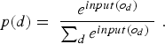
The objective of reinforcement learning problems is to find a policy that maximizes the sum of the so-called rewards over the total duration that the policy is applied for. For each time when a decision is made according to policy , the reward is defined as the net benefit occurring between and the time when the next decision is made. For the case study in this paper, the reward for the destination decision made by some policy is equal to the net cash flows obtained until the next destination is selected. In this sense, the framework used in this paper is closer to semi-Markov decision processes (Bradtke and Duff 1995) than to more commonly used Markov decision processes (Bellman 1957). Since finding the optimal policy is an optimization problem over functions, the class of functions that the optimization is performed over needs to be decided. For this paper, the policy class used for each of the three policies consists of a neural network. Neural networks were chosen due to their versatility in modelling arbitrary functions as well as the success of recent improvements in gradient-based methods for optimizing their parameters (LeCun et al. 2015; Schmidhuber 2015). In a machine learning context, neural networks are parameterized function architectures that can be viewed as layers of (partially) interconnected nodes. They are sometimes referred to as ‘artificial neural networks’ in order to distinguish them from the biological neural networks present in central nervous systems (from which they draw inspiration).

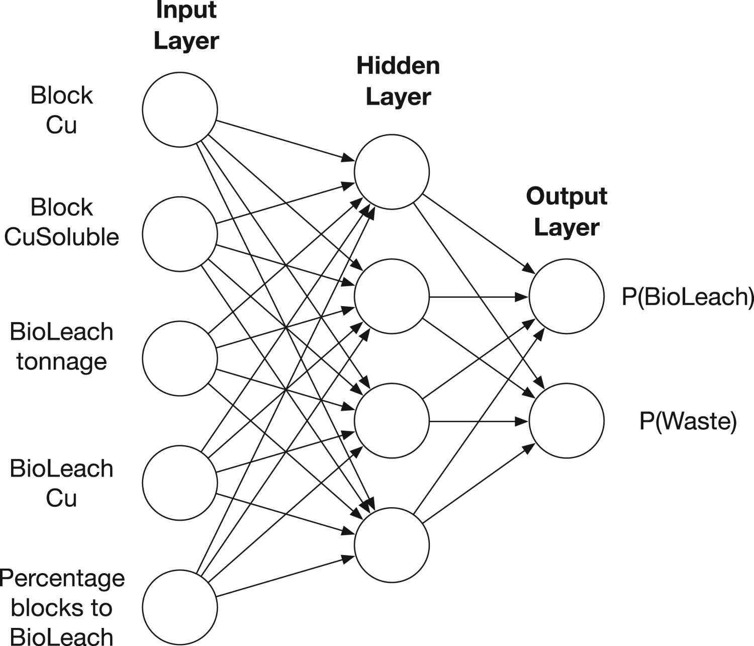
The neural network used for the BioLeachVsWastePolicy is illustrated in Figure 2. It is a feed-forward, fully-connected network with a single hidden layer. The circles in Figure 2 correspond to the interconnected ‘neurons.’ For illustration purposes, it should be noted that the number of hidden neurons in Figure 2 is much smaller than the number used in the experiments described in Section ‘Conclusions’, which used between 300 and 800 hidden neurons (depending on the size of the input layer). The input neurons correspond to the components of the state vector, and the two output neurons correspond to the probability that the optimal destination is or , respectively. In order for the policy to make a deterministic decision, the destination corresponding to the highest probability can be selected. Note that a single output node would have sufficed, since could have been computed as . However, the two-output network structure was shown because it better illustrates the type of multiple-output networks necessary when more than two destination decisions are considered.

Figure 2

Neural network representation for BioLeachVsWastePolicy. Images are available in colour online.

To compute for some state vector with components and some destination , the following steps are performed for this particular network:

[1] The input to each hidden neuron is a linear combination of the input neurons:

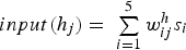
[2] The output of hidden neuron is determined by applying its activation function to its input. There are many possible choices for the activation function. This paper uses the simple rectified linear function (ReLU), which is generally regarded as a good choice for fully connected networks. The output using ReLU activation is computed as:

[3] The input to each output neuron , , is a linear combination of the outputs of the hidden neurons:

[4] The output of each output neuron is computed by applying the softmax function to its input:

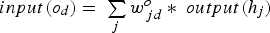
The networks used for the other two sub-policies are similar to the one for BioLeachVsWastePolicy, the only differences being that the input neurons will correspond to the appropriate state representation for the sub-policy considered. As such, the number of hidden neurons will differ in order to remain proportional with the number of input neurons, and the number of output neurons will reflect the number of destinations that the sub-policy chooses between.

Gradient-based policy optimization

This section describes the use of a policy gradient approach for optimizing the neural network policies. Policy gradient has first been proposed by Williams (1992), who also described how it should be used in conjunction with neural networks. However, neural policy gradient was seldom used until new developments in neural network training allowed it to obtain impressive results in difficult problems. For example, it was one of the building blocks for the widely acclaimed AlphaGo program (Silver et al. 2016).

Policy gradient updates the parameters of the policy by performing gradient ascent on the objective function. For the stochastic optimization problems in this paper, the objective function is an expected value and is not necessarily differentiable, so computing its gradient is non-trivial. Policy gradient addresses this by relying on the key insight that, given a function and a probability density function parameterized by , the following equality holds: (1) For policy gradient, corresponds to the objective function and corresponds to the decision selection (output) probabilities 4 computed by the neural network as described in Section ‘Policy representation’. The probabilities are parameterized by , a matrix containing the values and defining the linear combinations that are part of the neural network. The equation above circumvents the need for directly computing the gradient of the objective function. Instead, only the gradient of the action-selection probabilities needs to be computed. This is considerably easier, since neural networks are typically built in order to ensure differentiability and efficient gradient computation, whereas objective functions are not.

The optimization process starts with some initial policy, typically constructed by randomly initializing the weight matrix . The destination-selection process then interacts with the generative model described in Section ‘Determining plant output’ by taking the following steps every time a block needs to be allocated:

The reward (cash flow since the last decision was made) is computed.

The state vector components are determined according to the most recent information concerning material properties at different locations.

The state vector is used as an input to the corresponding sub-policy neural network, and a destination is selected according to the probabilities computed by the output nodes of the network, by deterministically picking the action with the highest probability.

The reward, state, and decision are stored in order to be used by the optimization process.

When the planning horizon is reached, the weights of the neural network are updated based on the rewards and decisions stored during the previous steps.

The updates at Step 5 are performed by taking a step in the direction of the approximate gradient of the objective function (expected total reward for the period of interest). The gradients with respect to different weights in the network are computed using backpropagation, a technique based on the chain rule that iteratively computes the gradients for each layer in a neural network, starting with the output layer.

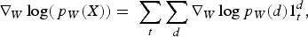
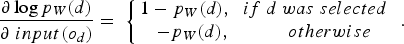
According to Equation (1), the gradient of the objective function can be written as a function of the gradient of the logarithm of the destination-selection probabilities. The gradient of this logarithm with respect to the output layer's inputs is Therefore, the gradient of with respect to each weight is:

Continuing applying the chain rule, one gets: Going back to Equation (1), the gradient of the objective function can be expressed as

As is common in stochastic gradient methods, the outer expectation in the equation above is replaced by a single-sample estimate, i.e. is replaced by , where is the net cash flow obtained during the planning horizon and is the vector of decisions that led to that cash flow. The gradient of can be computed as where the outer sum is taken over all decision times encountered during the planning horizon, the inner sum is taken over all the destinations, and is equal to 1 if destination was selected at decision time and zero otherwise.

From the above, a stochastic approximation for is obtained. This allows the use of stochastic gradient ascent in order to update the parameter matrix approximately in the direction of greatest increase in . The RMSPprop method (proposed by Geoff Hinton in Lecture 6 of CSC321 Winter 2014 at the University of Toronto), is used here, as it performs more complex updates than the alternative common stochastic gradient ascent approaches and provides increased stability and convergence speed. Denoting the stochastic approximation of 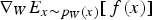by , RMSprop updates the weight matrix using the equations where and are user-defined parameters set to 0.99, 0.001 and 0.00001, respectively, for the case study in this paper.

This completes the description of step 5 above. The learning process involves repeating steps 1–5 until a pre-defined condition is met (for instance, a pre-defined number of iterations have been performed, or the network has achieved a satisfactory level of performance). Once the learning process is complete, the final values for the neural network weights determine the three sub-policies CrusherVsBioLeachVsWastePolicy, BioLeachVsWastePolicy and AcidLeachVsWastePolicy. Combining them results in an optimized policy for sending extracted material to the initial destinations. The policy determines the initial destination each extracted block should be sent to, including which of the crushers. The crushed material is placed on the conveyor belt corresponding to the plant with the lowest feed pile tonnage, similarly to the baseline policy.

The behavior of the policies is determined by the weights resulting from the optimization procedure described in this section. Unfortunately, while the use of neural networks allows us to express a very large class of policies and use efficient optimization techniques, it also renders the resulting policies very hard to interpret by a person. While there are tools that one can use to understand their behaviour (for instance, one could plot how the decision changes as the grade changes in a certain state), expressing a full neural network policy in a compact, human-readable form is, unfortunately, not possible.

Case study

The case study compares the baseline cut-off grade policy to the neural network based policy for the task of selecting the initial destination. The policies are compared according to the cash flows they obtain under scenarios generated using the joint uncertainty model described in Section ‘Determining plant output’. In order to conduct a fair evaluation, the 15 geostatistical simulations provided were divided into two groups. The first, consisting of 10 simulations, was used for optimizing the cut-off grades as well as the neural network parameters. The cut-off grades were optimized using a grid search, resulting in values of 0.52, 0.33 and 0.49 for , and , respectively. The neural network parameters were optimized using policy gradient reinforcement learning, as discussed in the previous section. The 5 remaining simulations were used for comparing the optimized cut-off policy to the optimized neural network policy. The policies’ behaviour was evaluated for a total of 6 months of production.

The rewards used by the reinforcement learning approach are the net cash flows obtained after processing and selling the extracted material. The objective function is the expected value of the total reward for a pre-defined period of time (in reinforcement learning terminology, a finite-horizon value function). For this case study, the length of this period of time was set to the 36 h after the material in the allocated block reaches its destination. The 36-hour window was chosen in order to account for the effect of the material in the block on cash flows given the different destinations’ throughputs and lags (e.g. feed pile-induced).

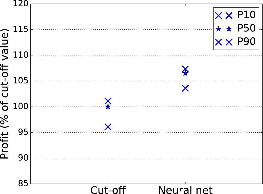
The net cash flow during a time period is computed as The value of is computed by multiplying the amount of copper produced according to the current scenario at each destination during period by the copper price and summing up the results over all destinations. The processing cost for each plant is computed as 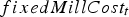where includes the fixed cost per unit of time of operating the mill regardless of the tonnage, and is a function of the tonnage processed during time and includes all the variable costs. For the heap leaches, only tonnage-dependent costs are considered. The value of was set to US$3 per 0.1% As content above 0.2% for each ton of concentrate processed during time . This value was chosen according to Bruckard et al. (2010), who averaged various sources. Finally, 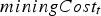denotes the cost of extracting and hauling material during time . The exact values of 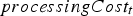and were provided by the mining complex and are omitted for confidentiality. Figure 3 compares the cash flow obtained for the test simulations by the baseline cut-off grade policy and the neural network policy. The P50 for the neural network policy is 6.5% higher than for the cut-off grade policy, and the P90 for the neural network policy is higher than the P10 for the cut-off policy.

Figure 3

Cumulative cash flow comparison between the cut-off grade policy and the neural network policy. The y-axis values indicate the percentage of the cut-off policy's value computed using the test simulations. Images are available in colour online.

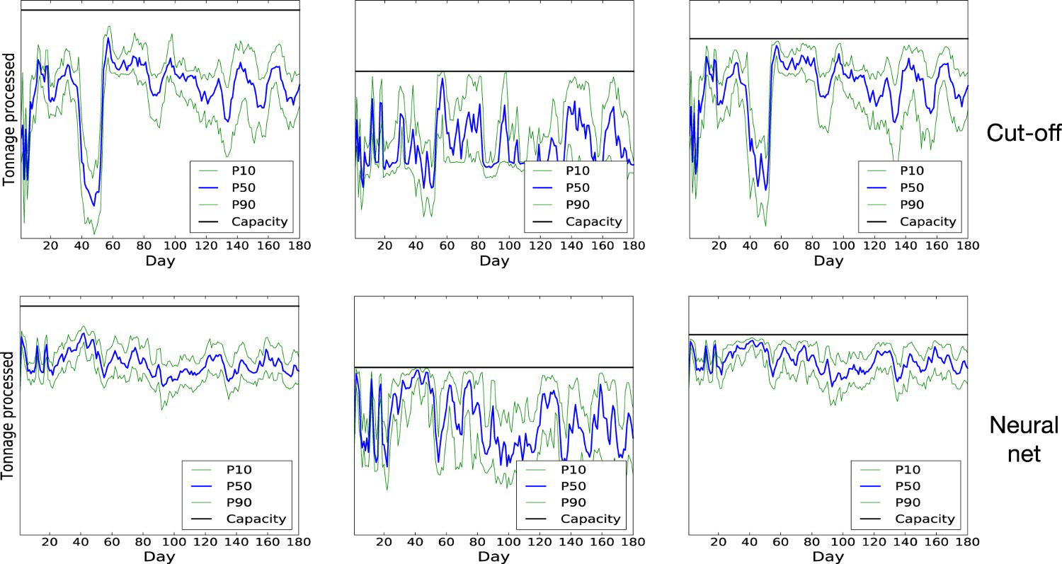
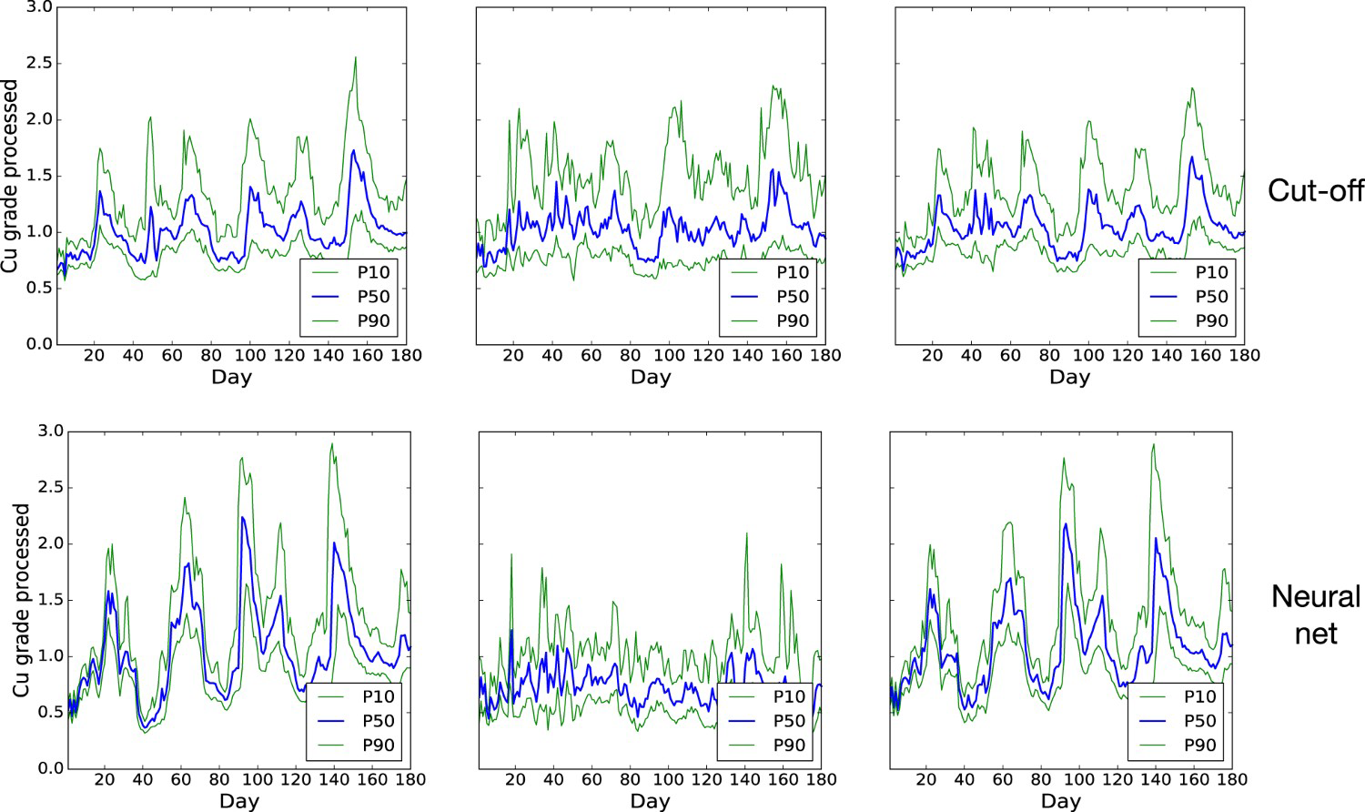
The difference between the two policies appears to be largely explained by the way they manage to ensure a constant feed for the plants. The component of the total processing cost, which is incurred irrespective of the tonnage processed during time , acts as an implicit penalty on feeding the plant below capacity. In Figure 4, it can be seen that the neural network policy does a better job at providing a consistent feed for the mill than the cut-off grade policy. Figure 5 suggests that this is because the cut-off grade policy is more flexible about the way it can adapt the grade of the material being sent to the plants. Indeed, it can be seen that, for periods corresponding to low plant tonnage under the cut-off grade policy, the neural network policy typically lowers the head grade to below the 0.52 cut-off. By contrast, in periods where high-grade material is abundant, the head grade is raised, which can reduce the time spent waiting for material to be crushed and processed and therefore improve shovel productivity.

Figure 4

Daily tonnage processed at the three plants when initial destinations are selected according to cut-off grade policy (above) and neural network policy (below). The tonnages are compared to the capacities (horizontal black lines).

Figure 5

Average daily grade processed at the three plants when initial destinations are selected according to cut-off grade policy (above) and neural network policy (below).

The example shown in Figure 6 gives further weight to this hypothesis. This case provides two situations in which the neural network policy selects a different destination from the cut-off grade policy. By considering inputs other than the grade, the neural network is capable of making more flexible decisions. In the top situation, where there is not much material sent to the crushers and the As concentration is lower, the neural network decides that the block should be sent to one of the plant crushers, despite having a lower grade than in the bottom situation. The cut-off grade policy does not have the flexibility to adapt its decisions to additional information in this way.

Figure 6

Two situations where the neural network decision is different from the cut-off policy decision. Images are available in colour online.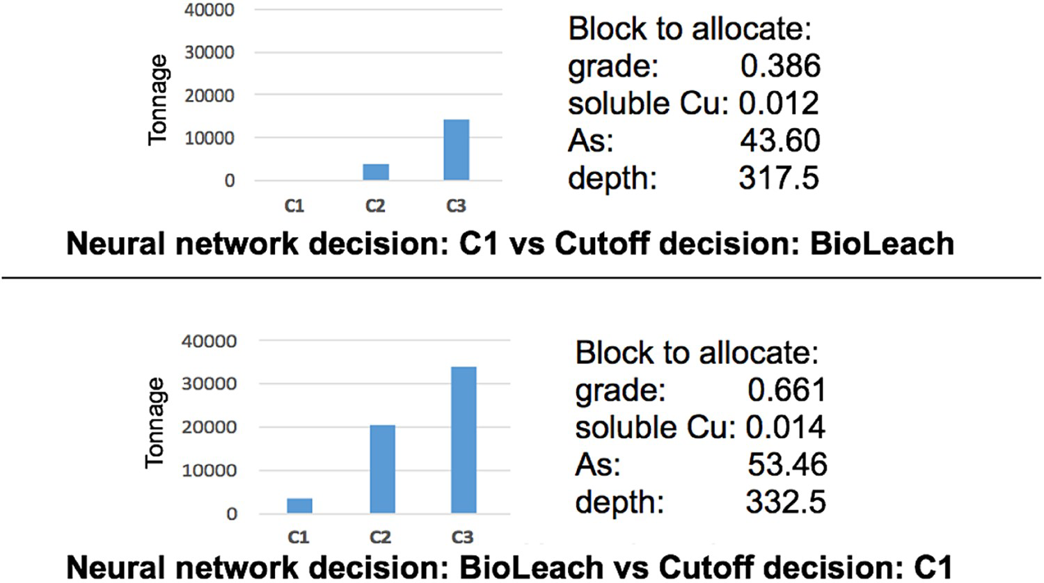

Conclusions

This paper demonstrates how to use reinforcement learning in order to compute policies for allocating material in a mining complex. The reinforcement learning allows new information to determine the policy's response by including that information into the state update process. The policy then returns the decision corresponding to the updated state. A key advantage of the reinforcement learning approach is that it can alleviate the need for computationally expensive re-optimization. There are two ways in which this happens. First, because the policy produced by reinforcement learning is a mapping from states to decisions rather than a sequence of decisions, there is no re-optimization necessary when new information is obtained. Instead, the policy only needs to compute the decision corresponding to the new state, which typically requires very little computational overhead. Second, if the distribution of the data used in the optimization process is carefully selected (Levine and Koltun 2013), the same policy can be used for different input distributions; for example, the same destination policy can be used for different extraction sequences. This can allow a reinforcement learning policy to be used as part of global mine complex optimization methods. For example, metaheuristic and hyperheuristic production scheduling methods (Lamghari and Dimitrakopoulos 2012, 2018) could use the costs and revenues obtained when applying the optimized policy for computing the objective function associated with a given perturbation, thus better informing the search for the optimal extraction sequence.

In addition to destination policies, the types of policies proposed here could be used for many parts of the mining complex, such as extraction (deciding which of the available blocks each shovel should extract next), fleet allocation, or processing. Allowing these policies to be optimized simultaneously could further improve coordination and final value, similarly to existing work on global optimization of mining complexes under uncertainty (Montiel and Dimitrakopoulos 2015; Montiel et al. 2016; Goodfellow and Dimitrakopoulos 2016, 2017). Incorporating very recent advances in reinforcement learning (e.g. Mnih et al. [2016]) could ensure that this is done as efficiently as possible. In order for the outcome of any optimization process to be successfully used in production, it is essential that the models used for the optimization closely match the behaviour of the actual process of interest. This requires careful assessment and validation of the model's assumptions and outcomes, which was not performed in this work but is crucial when moving from experimental development to actual deployment. In addition, policy parameters that were optimized based on some computational model could continue to be updated based on real data obtained during deployment. Another important avenue for future work is to explicitly incorporate particular sensors and data streams into the decision-making process. This may involve including the sensors directly as part of the state representation or building stochastic models that are updated based on new incoming data. Recent work by Benndorf and Buxton (2016) shows examples of this can be done.