
Abstract
Simultaneous stochastic optimization of mining complexes aims to optimize its different components in a single optimization model under grade, geometallurgical and material type uncertainty. The single optimization model capitalizes on synergies between the different components and the quantified variability and uncertainty of the materials mined, to better meet production targets while maximizing the net present value (NPV) of a mining complex. Integrating uncertainty and decisions about geometallurgical aspects of materials in the optimization model assists in achieving higher and more stable throughput with comminution circuits. This paper introduces an approach to integrate uncertainty and decisions about two non-additive geometallurgical properties, semi-autogenous power index and bond work index in the simultaneous stochastic optimization model. An application of the proposed approach at a large copper–gold mining complex indicates higher chances of meeting the different production targets, substantial increase in metal production and a 19.3% increase in NPV compared to the conventional plan.
Introduction
A mining complex consists of multiple components such as mines, crushers, stockpiles, leach pads, processing mills, waste dumps, means of transportation and customers. The components are interlinked to form the mineral value chain. Material extracted from the mines flows through the mineral value chain to finally produce the products which are delivered to customers and/or spot market. In the last decade, developments have been made to integrate different decisions in the mineral value chain in one single optimization model. The integrated model of a mining complex simultaneously optimizes the different decisions in the related mineral value chain to utilize synergies in developing jointly sequence of extraction, destination policies, processing stream utilization, operating modes, transportation alternatives, capital expenditure, and so on.
Past work in simultaneous optimization models of mining complexes can be categorized into two groups: conventional approaches and stochastic approaches. Hoerger et al. (1999) present a model for Newmont's Nevada mining complex that simultaneously optimizes the timing of open-pit layback, underground stope development, capital expenditure, the timing of processing plant startup and shutdown, and, material routing decisions. Stone et al. (2007) present BHP's advance mine planning optimization tool, ‘Blasor’, which simultaneously optimizes long-term panel extraction sequence and amount of material extracted from multiple mines. Whittle and Whittle (2007) present a global asset optimization model that includes optimization of extraction sequence, mining rate, cut-off grade policy, processing path selection, stockpiling strategy to satisfy production targets. The model does not optimize the different components simultaneously instead repeatedly creates random feasible extraction sequence and finds a locally optimal blending and processing stream utilization strategy. Whittle (2018, 2014) presents the Prober C algorithm that generalizes the algorithm used to solve global asset optimization model. In Prober C, grades are expressed as an additive quantity, say metal quantity. This structure allows integrating aspects of stockpiling, transportation, and so on in the global asset optimization model. An integrated approach is presented by Pimentel et al. (2010) to address the simultaneous optimization of mining complexes and possible solution strategies. Some of the typical limitations of the conventional approaches include: (i) aggregation of mining blocks into larger volumes, before starting the optimization process, to reduce computation requirements, (ii) do not simultaneously optimize the different components of mining complex, i.e. separate model for different components of mining complexes that interact through some form of heuristic approach, (iii) do not consider uncertainty in grade, geometallurgical and material types of the mineral deposits.
Simultaneous stochastic optimization of mining complexes overcomes the above limitations of earlier models by considering one single optimization model to simultaneously optimize the different components of a mining complex under uncertainty. Montiel and Dimitrakopoulos (2015) propose a model that simultaneously optimizes block extraction, block destination, processing streams utilization, operating modes, transportation alternatives, under grade and material type uncertainty. Results from a copper–gold mining complex indicate deviations of less than 3 and 1.2% from capacity and blending targets respectively for the proposed model compared to large and impractical deviations in the range of 30–40% and 11–22%, respectively, in the conventional mine production plan (Gemcom, 2005). In addition, the proposed method increases the net present value (NPV) by 5% as compared to conventional mine production plan. Montiel et al. (2016) extend the model to include underground mines. Montiel and Dimitrakopoulos (2018) present another extension integrating the specification of additional practical operational constraints to mine production schedules, as well as a large-scale application and comparisons with conventional methods at the Twin Creeks gold mining complex, Nevada. Montiel and Dimitrakopoulos (2017) present a metaheuristic algorithm to solve the large optimization model of mining complexes. The algorithm first changes the block extraction and destination decisions to improve NPV and then selects the optimal operating and transportation modes. The decisions are synchronized as the algorithm progresses. The proposed method increases the NPV by 30% and decreases the deviation from production target by 45% compared to conventional mine production plan. Goodfellow and Dimitrakopoulos (2016) present a model that simultaneously optimizes block extraction decisions, multiple element destination policies, and processing stream utilization strategies, under grade and material type uncertainty. The proposed method is applied at a copper–gold mining complex and shows deviations of less than 10% compared to 40% in the conventional mine production plan while increasing the NPV by 22.6%. Goodfellow and Dimitrakopoulos (2017) study the efficiency of the multiple element destination policies. Results from a nickel-laterite mining complex show deviation of less than 1% for blending target and improved NPV of 3% for multiple element destination policies under supply uncertainty compared to multiple element destination policies for estimated deposits. Some of the common and useful aspects of simultaneous stochastic optimization models of mining complexes can be summarized as: (i) ability to capitalize on synergies between different components of mining complexes, (ii) capability to take advantage of and capitalize on the variability of grade and material type, (iii) do not aggregate mining blocks into large volumes to misrepresent mining selectivity, (iv) focuses on value of product sold to the different customers instead of value of mining blocks, (v) increased expectation of meeting production forecasts, and, (vi) higher NPV and metal production.
The stochastic mine planning models reviewed above although incorporate grade and material type uncertainty, but, do not integrate the uncertainty and variability related to geometallurgical properties of the material. Geometallurgical properties such as grinding ability\hardness of material processed, ore texture, and so on, affect the throughput and energy consumption of the comminution circuits. Not accounting for such geometallurgical aspects in strategic mine planning models may result in sub-optimal mine plans (Dowd et al., 2016). More specifically, comminution circuits in a mining complex typically account for 33–50% of the mine costs (Curry et al., 2014), which depends on factors such as the feed particle size, hardness of the material and many more. Ballantyne and Powell (2014) present a survey of the comminution circuit energy consumption of major Australian gold and copper producer which account for 1.3% of Australian electricity consumption. The hardness of the material is measured using grindability tests such as semi-autogenous (SAG) power index (SPI) for SAG mills and bond work index (BWI) for ball mills. Verret et al. (2011) present the overview of the different grinding ability tests used characterizing ore hardness for comminution circuits. Hardness indexes such as SPI and BWI are hard to model due to their sparse sampling nature. Different approaches are proposed to model geometallurgical properties such as primary and secondary response framework (Coward et al., 2009), combination of simulation and power approach (Alruiz et al., 2009), use of two-stage linear regression model (Boisvert et al., 2013), projection pursuit method (Sepúlveda et al., 2017), and fuzzy clustering (Sepúlveda et al., 2018). However, it is even harder to include the hardness indexes such as SPI and BWI in the strategic mine planning models due to their non-additive nature. In addition, blending of material with substantially different hardness properties can introduce the problem of inconsistent throughput and higher energy consumption in the comminution circuits.
The work presented herein introduces an approach to integrate geometallurgical uncertainty of two hardness indexes SAG power index (SPI) and bond work index (BWI) into the simultaneous stochastic optimization model of mining complexes. In addition, the proposed model also deals with the blending of multiple materials with different hardness properties to ensure consistent throughput of material to comminution circuits. In the following sections, a brief description of the extended model of Goodfellow and Dimitrakopoulos (2016) is provided, followed by an application at a large copper–gold mining complex that consists of 2 mines with 12 different material types, 5 crushers, 2 stockpiles, 3 processing mill, 1 waste dump and, 2 leach pads, and produces copper, gold, silver and, molybdenum products. Conclusions and future work follow.
Method
This section discusses the model for simultaneous optimization of mining complexes under uncertainty proposed in Goodfellow and Dimitrakopoulos (2016), which is extended in this work to include uncertainty and constraints related to geometallurgical properties associated with grindability (SPI and BWI). Geometallurgical properties are non-additive in nature and this specific aspect is not accounted for in Goodfellow and Dimitrakopoulos (2016). The work presented herein provides an approach to include constraints and uncertainty related to such non-additive geometallurgical properties in the context of simultaneous optimization of mining complexes. In addition, and most importantly, the work presented highlights the applied aspects of the method with an application at a large copper–gold mining complex with over 1.6 million binary and 50,000 continuous variables. First, definitions and notation are provided, then, the different decision variables are discussed. Finally, the objective function and constraints are outlined.
Definitions and notation
The notations used in this section are as follows.  represents a group of mines.
  represents the set of mining blocks
 for mine
  and
and  represents the mining cost of block
  in period
  . A block
  is accessible to extract following the extraction of its overlying blocks represented by a mathematical ‘Set’
  .
.  denotes a set of scenarios that quantify the joint uncertainty in grade, geometallurgical properties and material types.
  represents the scheduling periods. Extracted material from mines can either be stockpiled, or, processed after crushing, or sent to waste.
  , represent the amount of property
 at location
 in period
 and scenario
 . S, represent the set of stockpiles.
 represents the stockpiling cost of stockpile
 for property
  in period
  .
.  represents the cost of re-handling material from stockpile
 for property
 in period
 .
.  represents the set of crushers.
  represents the crushing cost of material with crusher
  for property
  in period
  .
.  represents the set of processing mills.
  represents profit (selling price–selling cost) for recovered product a with processing destination
  in period
  .
. represents the processing cost with processing destination
  for property
  in period
  . Properties such as metal tonnage, rock tonnage and ore tonnage are represented by
 , and are calculated by adding amount of metal, rock, and ore tonnage processed at different location in a mining complex. Properties such as head grade copper, head grade arsenic, etc. are calculated as head grade copper is equal to total copper metal tonnage/total ore tonnage, head grade arsenic is equal to total arsenic metal tonnage/total ore tonnage respectively at different locations.
  represents the amount of different products recovered.
Production targets are usually present in a mining complex, such as (i) capacity targets represent by a set  , (ii) quality targets represented by a set
  , and (iii) geometallurgical targets represented by a set
  . Mineability targets are also included in the model. Mineability targets ensure that the production schedules are practically mineable.
  is the specified mining width.
  is the number of blocks scheduled in multiple periods inside a mining width.
  is the penalty cost associated with not scheduling blocks inside the mining width in the same mining period.
  and
and  represent the penalty costs with deviations from maximum/upper and minimum/lower production targets respectively for property
  in period
  . Profits and costs are discounted using an economic discount factor
  , as
, as  . Cost of deviation from capacity, blending, geometallurgical and mine ability targets are also discounted using a geological discount rate
  , as
, as  used from Dimitrakopoulos and Ramazan (2004), Ramazan and Dimitrakopoulos (2013), and Spleit and Dimitrakopoulos (2017). Geological risk discounting helps to defer the risk of not meeting production targets to later years when more information will be available.
Decision variables
Decision variables for the model are: (i) mine extraction sequence variables  defines whether (1) or not (0) block
  is extracted in period
  , (ii) processing stream utilization variables,
  define the proportion of material sent from location
  to subsequent location
  in period t and under scenario
  , and (iii) cluster destination policy variables
 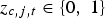 define whether (1) or not (0) cluster
  is sent to one of the allowed destination
  in period
  . Cluster destination policy is based on clusters defined over multiple elements of interest (Goodfellow and Dimitrakopoulos, 2016). Continuous variables that allow deviations from different targets are also included in the model. Surplus variable
  represents excess from maximum target (
 ) for property
  in period
  and scenario
  . Shortage variable
  represent shortage from minimum target (
 ) for property
  in period
  and scenario
  .
.
Objective function
The objective function (Equation (1)) of the model is a two-stage function that maximizes the value of the product generated from a mining complex and delivered to customers or spot market, while minimizing the deviations from capacity, blending, geometallurgical and mineability targets, under grade, geometallurgical and material type uncertainty.
Part I in the objective function represents the profits of different products produced and sold to the customers. Part II is the processing cost of the material at the different processing destinations. Part III represents the crushing cost at the different crushers. Part IV represents the stockpiling cost at the different stockpiles. Part V represents the cost of re-handling material from the different stockpiles. Part VI, VII, and VIII represents the cost of deviation from the capacity, quality and geometallurgical targets at the processing streams. Part IX is the cost of deviation from the crusher capacity target. Part X is the cost of deviation from the stockpile capacity target. Part XI represents the cost of deviation from the mining capacity target. Part XII represents the mining cost at the different mines. Part XIII is the cost associated with the smoothness of schedules.
Constraints
The processing mill in the mining complex has multiple operating modes. Operating modes are defined herein as the configuration of the processing mill that determines the grinding size of the materials. For example, fine grinding compared to coarse grinding operating mode. Different operating modes have different costs, energy consumption, and throughput. However, such cost, energy consumption, and throughput for a fixed operating mode might change based on the hardness of material processed. For example, the fine grinding of hard material will require longer residence time when compared to the softer material, which results in higher costs and lower throughput. Uncertainty about the hardness of material results in inconsistent throughput, energy consumption, and operating cost with a fixed operating mode at the processing mill. Hardness index such as SPI and BWI are non-additive properties which cannot be directly included in the outlined optimization model. A different approach is utilized in this work to overcome such non-additive issues with hardness indexes. First, the operating mode is fixed and linked to the proportion of hard and soft material that the processing mills can process to achieve maximum throughput and recovery, and minimum cost. Such proportions of hard and soft material are defined as geometallurgical targets  with the different processing mills for a fixed operating mode. Further, the material at the mine is characterized as soft and hard material based on their hardness indexes. For instance, if the hardness indexes of the mining block in the mine are above a threshold, it is defined as hard otherwise soft.
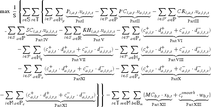
The amount of hard and soft material is extracted from the mine and sent to different processing streams and is finally processed at the different processing mills. At the different processing mills, the total amount of hard and soft material is determined, and their ratio is calculated as  . Finally, deviations from upper and lower limit of predefined geometallurgical targets
  , is calculated using Equations (2) and (3). Such deviations are penalized in the objective function with a penalty cost. Penalizing such deviations ensures that proportion of hard and soft material processed at the processing mills is within the required geometallurgical targets.
Equation (4) calculates the number of blocks scheduled in multiple periods ( ) inside a mining width given by
  and penalizes with a penalty cost of
  in the objective function. Other constraints implemented in the model are capacity/quantity, blending/quality, destination policy, processing stream flow, reserve, and slope, constraints detailed in Goodfellow and Dimitrakopoulos (2016).
Solution approach
The simultaneous stochastic optimization model of mining complexes outlined in the previous sections is a large combinatorial optimization model with millions of binary decision variables. Such large optimization models cannot be solved with general purpose commercial solvers such as CPLEX. Metaheuristic algorithms have proven effective to generate near-optimal solutions in reasonable computational time. The solution approach used to solve the model is adopted from Goodfellow and Dimitrakopoulos (2016, 2017). A brief review of the solution approach is outlined in Appendix A2.
Application at a large copper–gold mining complex
This section outlines the application of the method presented in the previous section at a large copper–gold mining complex and demonstrates its applied aspects. The management of the mining complex makes decisions based on a given strategic mine plan. The strategic mine plan currently used at the mining complex is developed with high-end conventional technologies as outlined in Section ‘Conventional optimization’. The framework proposed herein generates a stochastic strategic mine plan that accounts for variability and uncertainty in the supply of material and jointly optimizes the different components of the mining complex. The following sections compare and highlight the differences between the forecasted performance of the conventional and stochastic mine plans. The key aspect of the comparison is to highlight that the decision makers will make different decisions with the conventional mine plan as compared to the stochastic mine plan.
Overview of the copper–gold mining complex
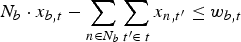
The copper–gold mining complex consists of two mines (Mine A and Mine B) with 120,000 and 78,000 blocks, respectively, and measure 25 × 25 × 15 Flow of material at the copper–gold mining complex. in size. The mineral deposits consist of 8 different mine zones, 8 different alterations and 10 lithologies each of the two mines. The stratigraphic sequence of material is waste rock, followed by copper oxide, mixed and copper sulphide. The mining complex produces copper concentrate and copper cathode as primary products and gold, silver and molybdenum concentrate as secondary products. The material extracted from both mines is classified into 12 different material types for each mine and can be sent to one out of 9 different destinations (5 crushers, 2 stockpiles, 1 bio leach pad (sulphide leach pad) and 1 waste dump) as shown in Figure 1. Material from five different crushers is further sent to three different processing mills and an oxide leach pad that supplies material to the port and to a copper cathode plant. The primary product generated at the port is copper concentrate. In addition, different secondary products such as gold concentrate, silver concentrate, and molybdenum concentrate are also generated at the port.
Copper cathode plant generates copper cathode as the product. The port and the copper cathode plant produce the final products of the mining complex which are transported and sold to different customers. Geometallurgical targets related to hardness indexes SPI and BWI are present with the three processing mills in the mining complex. Different blending and capacity targets are also present with the different components of the mining complex.
Stochastic optimization
The stochastic optimization model generates the stochastic mine production plan which is referred to herein as ‘stochastic plan’. The different parameters associated with the stochastic plan are discussed in Sections ‘Stochastic orebody simulations, Economic and operational parameters, Production targets, Metaheuristic parameters’.
Stochastic orebody simulations
Fifteen stochastic simulations are generated for each mine that quantifies uncertainty in grade, geometallurgical properties and material types using the direct block simulation with minimum/maximum autocorrelation factors (Boucher and Dimitrakopoulos, 2009). A brief review of the above simulation method can be found in Appendix A1. Grade uncertainty is quantified for seven different correlated properties namely: copper soluble (CuS), copper total (CuT), iron (Fe), arsenic (As), gold (Au), silver (Ag), and molybdenum (Mo).
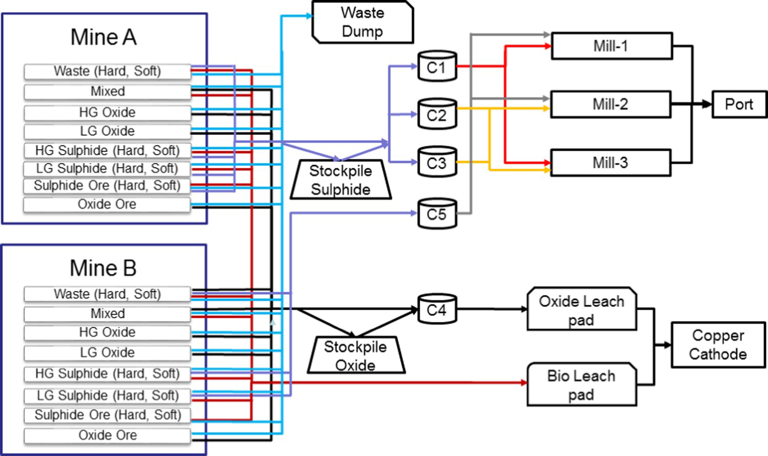
The two mines have eight different mine zones each, thus the simulation of grade properties were generated separately for each mine zone of each mine, each time using the samples of the seven correlated grade properties within the corresponding mine zone. The direct block simulation method was used to generate the correlated grade properties of the mining blocks within each mine zone. The combination of the simulated mining blocks from different mine zones provided the final simulation of correlated grade properties for each mine. Figure 2 represents the randomly selected three simulations for the two deposits for copper total grade property compared to the estimated deposit. Variability in copper total grade property can be easily perceived from the simulations compared to a smooth representation of the estimated deposits. Geometallurgical uncertainty is quantified for two hardness index values, SPI and BWI. The two mines have 10 different lithologies each, thus the simulation of geometallurgical properties were generated separately for each lithology of each mine, each time using the samples of SPI and BWI within the corresponding lithology. The direct block simulation method was used to generate the correlated geometallurgical properties of the mining blocks within each lithology. The combination of the simulated mining blocks from the different lithologies provided the final simulation of correlated geometallurgical properties for each mine.
Simulation of copper total for the two deposits compared to the estimated deposits.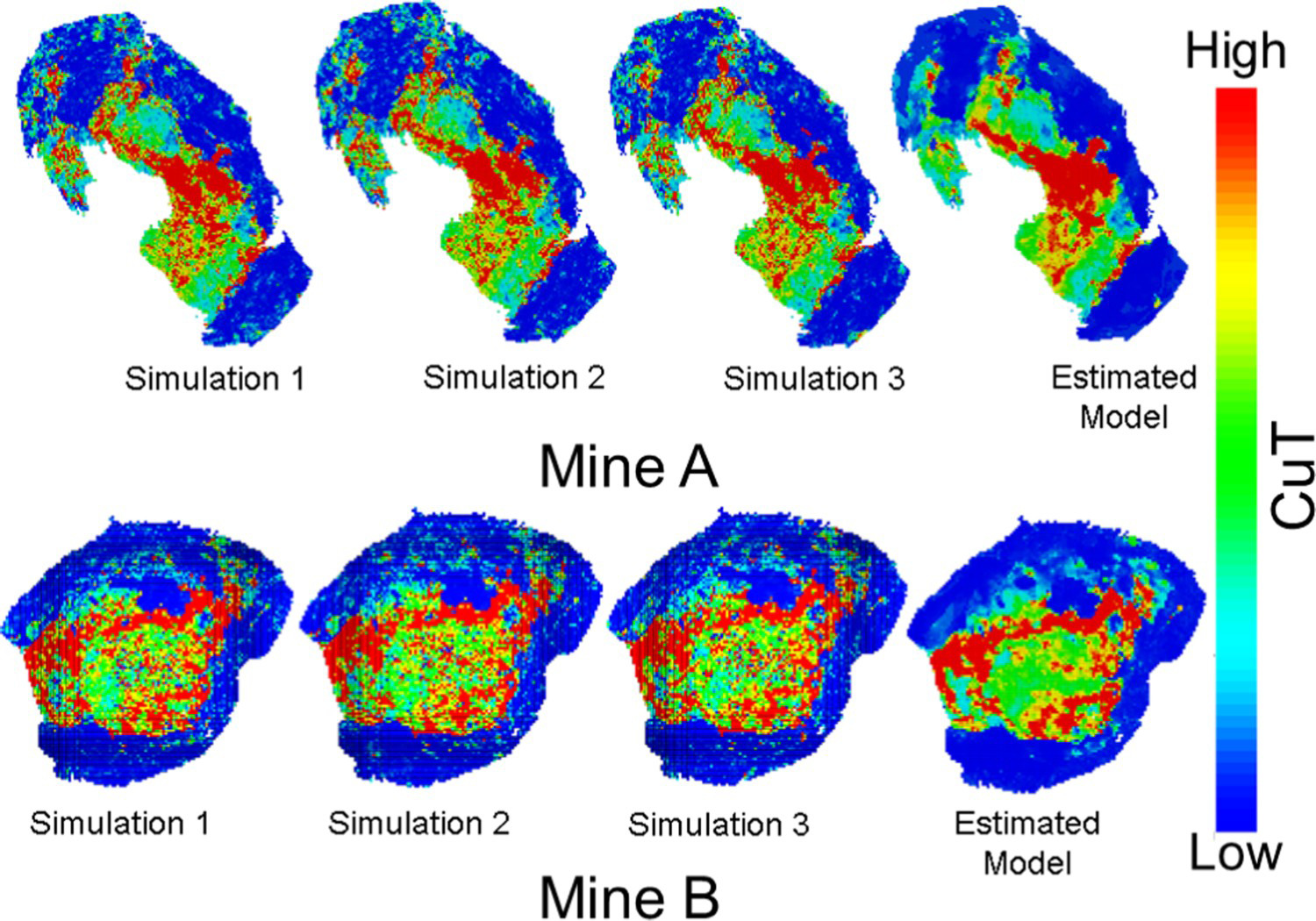
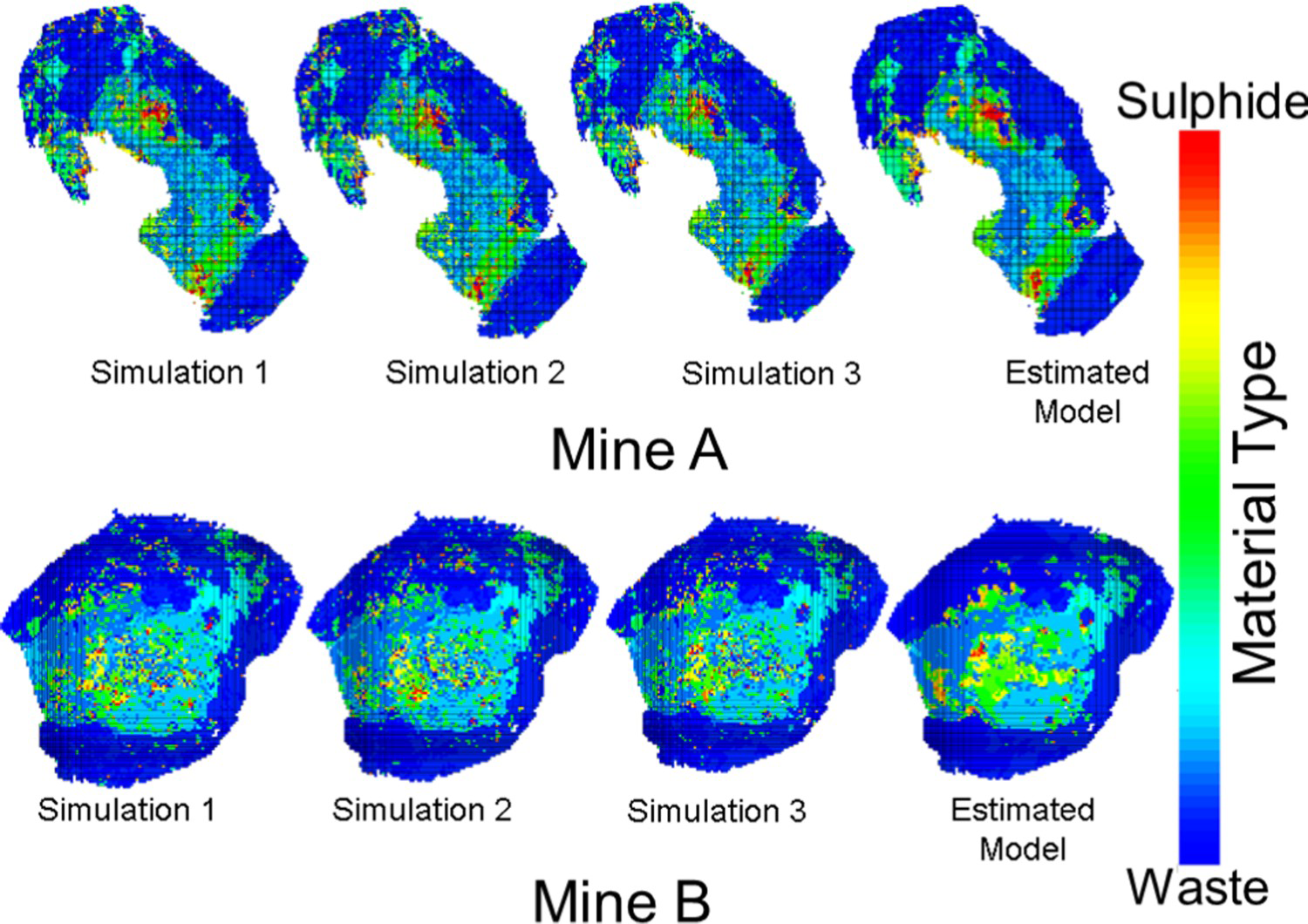
Figure 3 represents the randomly selected three simulations for the two deposits for the hardness index SPI compared to the estimated deposits. Large variability in hardness properties is perceived from the simulations compared to a very smooth representation of the estimated deposits. Variability and uncertainty in the grade and geometallurgical properties result in an uncertainty in material types which is shown in Figure 4. Materials are first classified as sulphide, oxide, waste and mixed based on geological properties (alteration and lithology) and grade properties (copper soluble, copper total, and copper soluble to copper total ratio), then geometallurgical properties (SPI and BWI) are used to further characterize the materials as soft and hard. Such classification strategy results in twelve different material types with distinct geological, grade, and geometallurgical properties. Material type uncertainty is quantified for twelve different material types (i) soft waste, (ii) hard waste, (iii) mixed, (iv) high grade oxide, (v) low grade oxide, (vi) soft high grade sulphide, (vii) hard high grade sulphide, (viii) soft low grade sulphide, (ix) hard low grade sulphide, (x) soft sulphide ore, (xi) hard sulphide ore, and (xii) oxide ore.
Simulation of SPI for the two deposits compared to the estimated deposits. Uncertainty in material types for the two deposits compared to the estimated deposits.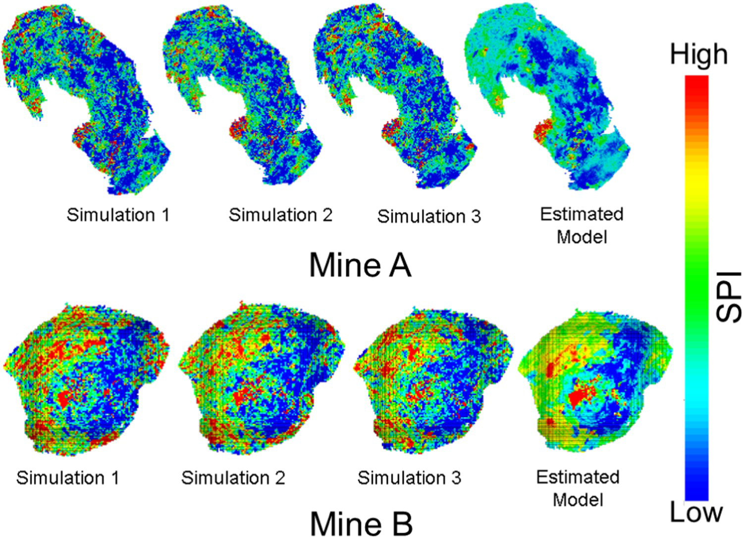
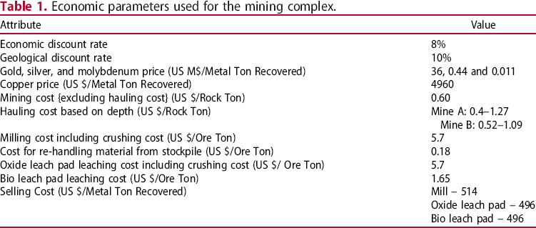
Economic and operational parameters
Economic parameters used for the mining complex.
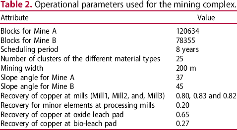
Operational parameters used for the mining complex.
Production targets
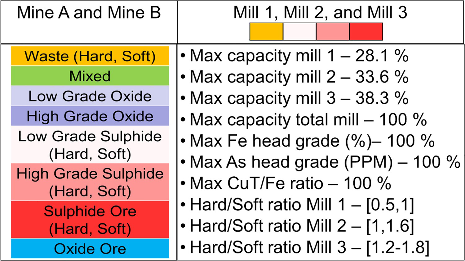
Figures 5 and 6 represent the different quality, quantity, and geometallurgical targets of the different processing streams in the mining complex. The colour legend represents the different rocktypes in the two mines, and the different processing streams have an associated colour band that shows what rocktypes are eligible to be processed at that processing stream. The geometallurgical targets mentioned in Figure 6 were selected based on the information provided by the mining company operating the mining complex. The mining complex has decided such targets based on studies about the configuration and operating modes of their different processing mills to achieve optimal throughputs. The modelling of hardness properties can also be integrated in the model by associating material to throughput and cost based on their hardness properties. However, the approach outlined in this work is selected to adhere to the specification and targets provided for the specific case study and the given mining complex. The different quantity and quality targets are scaled values for reasons of confidentiality.
Quantity and quality targets with crushers, stockpiles, and leach pads used for the mining complex. This image is available in colour online at https://doi.org/10.1080/25726668.2019.1575053. Quantity, quality, and geometallurgical targets with processing mills used for the mining complex. This image is available in colour online at https://doi.org/10.1080/25726668.2019.1575053.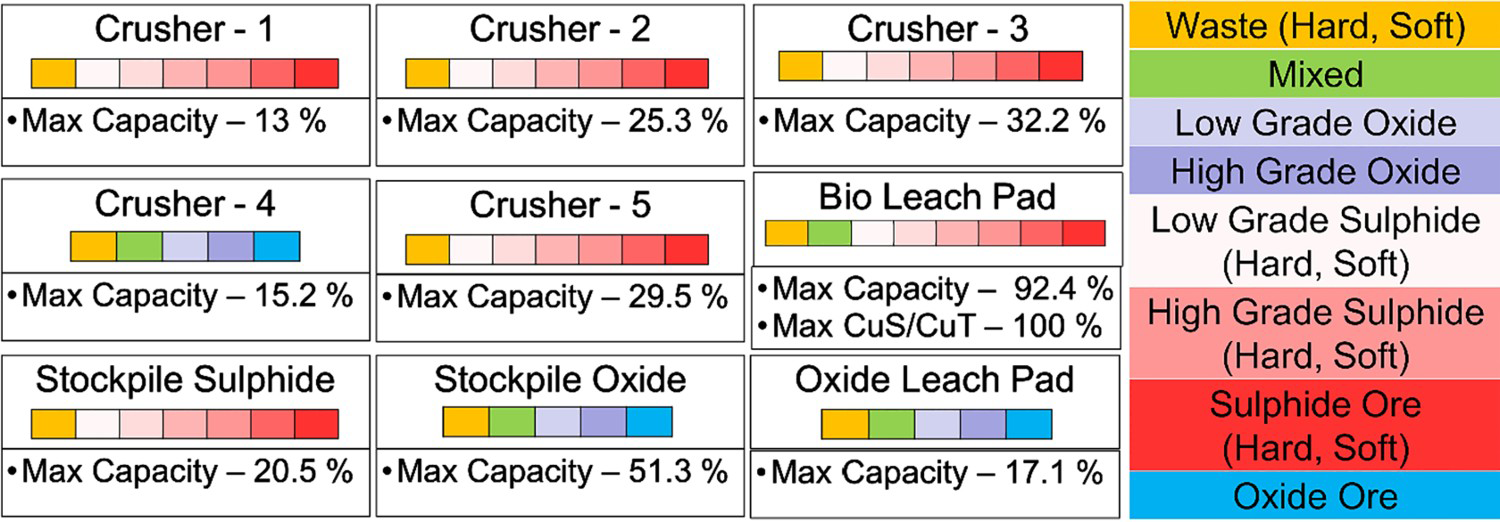
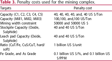
Penalty costs used for the mining complex.
Metaheuristic parameters
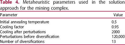
Metaheuristic parameters used in the solution approach for the mining complex.
Conventional optimization
The long-term mine production plan currently used at the mining complex is optimized using a two-step optimization approach by (a) the extraction sequence of multiple mines is optimized independently of each other using Whittle version 4.5.4 (Gemcom, 2005; Dassault, 2017), a widely used software for strategic mine planning, (b) the destination of the extracted material based on cut-off grade policy presently used at the mining complex and is based on Lane's approach (Lane, 1988; Rendu, 2014; Khan and Asad, 2018), and then defining utilization of different processing streams using a separate optimization model. In addition, this two-step optimization process is performed over the estimated mineral deposits, as is the standard practice in the mining industry. This long-term mine plan of the copper–gold mining complex generated with this two-step approach generates the conventional mine production plan, which is referred to herein as ‘conventional plan’. Economic parameters, operational parameters and production targets used to generate the conventional plan are same as the one used for the stochastic plan. The different geometallurgical and quality targets are only used during optimization of the processing stream utilization decisions in the conventional mine plan. The extraction sequence and cut-off grade policy in the conventional mine plan accounts only for the quantity targets. Estimated mineral deposits used in the conventional plan are shown in Figures 2 and 3 for grade and geometallurgical properties respectively. Material types of the estimated mineral deposits are shown in Figure 4.
Results of stochastic optimization and comparison to conventional optimization
The results of the stochastic optimization of the copper–gold mining complex are presented in this section. Results are reported using the 10th, 50th, and 90th percentiles risk profiles (P10, P50, and P90, respectively) of the different performance indicators with respect to the simulated orebody models of the two mines. P10 stands for the 10% probability that the values are below this value, P50 is 50% probability of having values below this value and, similarly, P90 stands for 90% probability of having values below this value. The forecasts of the stochastic plan are compared to the forecast of the conventional plan throughout its presentation and discussion, to highlight the differences in forecasted performance between the two mine plans and to show the added value of the stochastic framework, where appropriate.
Capacity targets
Figures 7(a–h) present the risk profiles of meeting the capacity target for crushers 1, 2, 3, 4 and 5, and mill 1, 2, and, 3. Figure 7(a) shows that the stochastic plan better utilizes and respects the crusher capacity (P10, P50, and P90 of the risk profiles are very close to the capacity target). The capacity target is only violated slightly in year 7, but is, overall, well controlled throughout the scheduling period in the stochastic plan (Figure 7(a)). Similar behaviour is observed for the stochastic plan for crusher 2 (Figure 7(b)), crusher 3 (Figure 7(c)), and crusher 5 (Figure 7(e)), where the capacity target is well respected and utilized over all the scenarios and throughout the scheduling period. However, the conventional plan shows very low production in year 6 for crusher 1, crusher 2, and, crusher 5. In addition, the production for crusher 2, and crusher 3 is lower throughout the scheduling period in the conventional plan (Figure 7(b,c) respectively) compared to the stochastic plan.
Forecasts for crushers 1–5 and capacity targets for the stochastic and conventional plans for mills 1–3.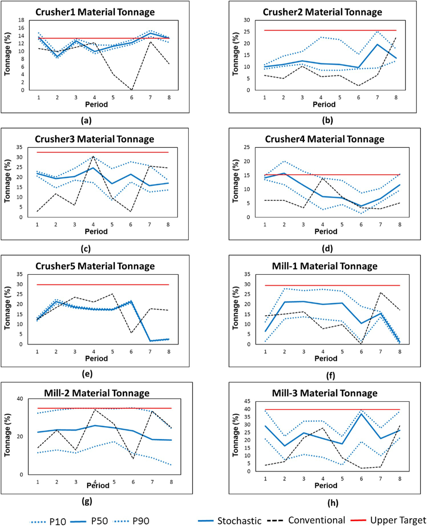
Crusher 4 (Figure 7(d)) shows only a small violation of the capacity target in the stochastic plan in year 2, but it utilizes the crusher 4 capacity better than the conventional plan. However, the risk profile for the stochastic plan for crusher 4 has a much wider envelop compared to the other crushers. Similar behaviour is present for mill 1 (Figure 7(f)) and mill 2 (Figure 7(g)) for the stochastic plan. Such a wide risk envelop in crusher 4, mill 1 and mill 2 capacity target originate from the processing of materials from both the mines, which results in a relatively high grade, geometallurgical and material type uncertainty. In the conventional plan, the capacity target is respected for crusher 4 (Figure 7(d)) but does not utilize the maximum crusher capacity. Similarly, the mill capacity is not fully utilized in the conventional plan for mill 1 and mill 2 with almost negligible production in year 6 for mill 1 (Figure 7(f)) and mill 2 (Figure 7(g)). The mill 3 (Figure 7(h)) capacity target has a relatively narrow risk envelop compared to the other mills because it processes material from only one mine. The stochastic plan better utilizes the capacity target in mill 3 compared to the conventional plan, where the production is almost negligible for the conventional plan in year 1, 6 and 7 (Figure 7(h)). Both the conventional and stochastic plan respect the capacity target of all the mills throughout the scheduling period.
Figure 8(a–d) presents the risk profiles of the capacity target for the oxide leach pad, bio-leach pad (sulphide leach pad), sulphide stockpile and oxide stockpile. A small violation only in year 2 is observed in the stochastic plan for oxide leach pad capacity target (Figure 8(a)) with a wide risk envelop originating from the reason explained above. The capacity target is well respected for the bio-leach pad (Figure 8(b)), stockpile sulphide (Figure 8(c)), and stockpile oxide (Figure 8(d)) in the stochastic and conventional mine plans. Figure 8(e–f) presents both the forecasted mining rates of the stochastic and conventional mine plans for mines A and B, respectively. The mining rates and, consequently, the mine production plans between the two mines are very different; more specifically, the stochastic mine plan mines more materials from mine A and less materials from mine B during the initial periods, when compared to the conventional mine plan.
Forecasts for sulphide stockpile, oxide stockpile, oxide leach pad, bio-leach pad capacity target, and mining rate of mines A and B for the stochastic and conventional plans.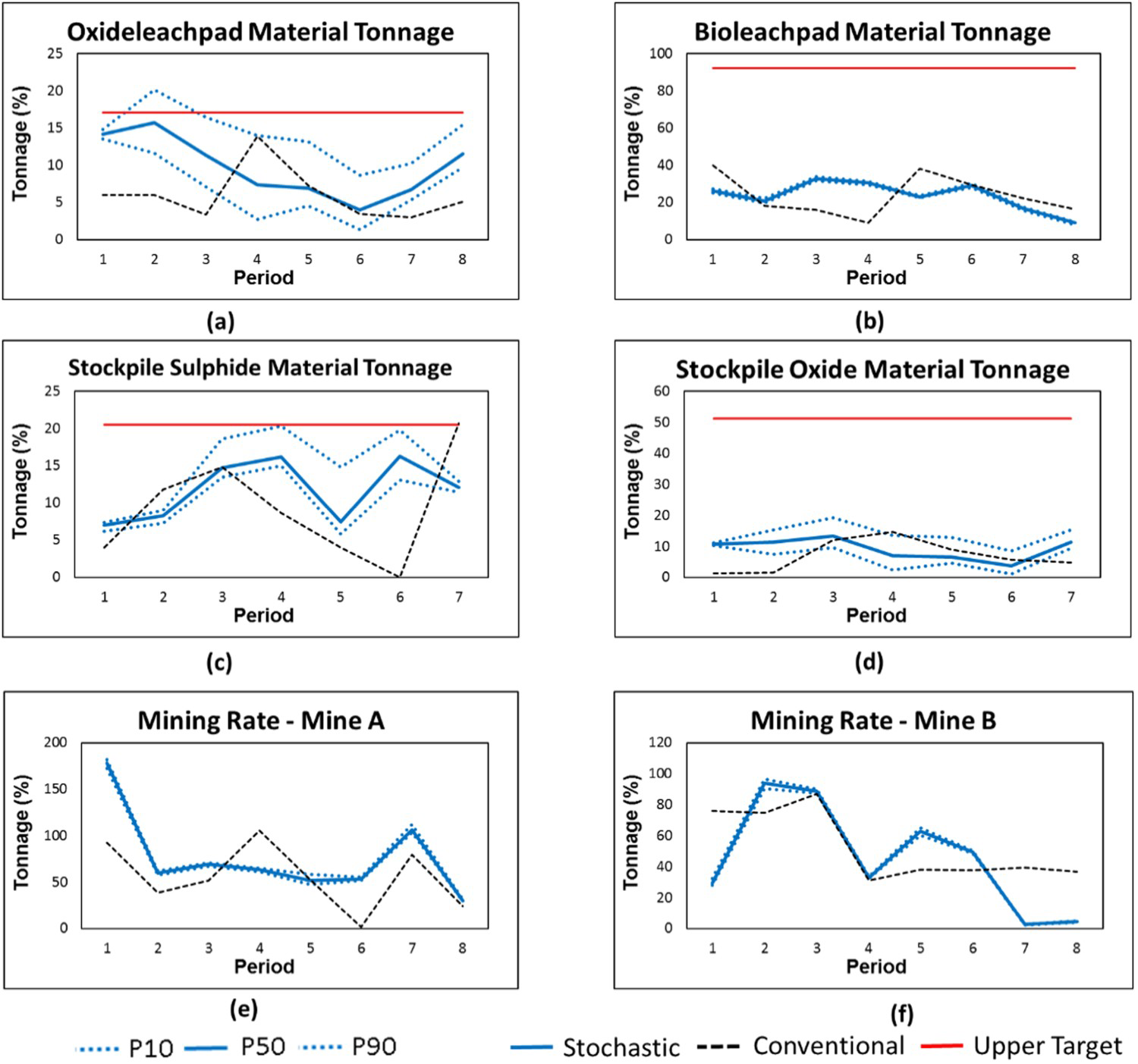
Blending targets
Figure 9(a–d) represents the risk profiles of blending target of (copper total to iron ratio) at the different processing mills and (ratio of copper soluble to copper total) for the bio-leach pad. The blending target is very well respected for the stochastic plan for mill 1 (Figure 9(a)), mill 2 (Figure 9(b)), and mill 3 (Figure 9(c)) with minor violations in years 2 and 4. The conventional plan shows larger violations from such target for all the mills. The blending target with bio-leach pad is very well respect in the stochastic and conventional plan. Figure 10(a,c,e) shows the risk profile of iron (Fe) head grade target for the different processing mills. The stochastic plan has a small violation for the iron head grade target for mill 1 (Figure 10(a)) in year 6. Mill 2 (Figure 10(c)) presents a small violation in year 6 for the iron head grade target in the stochastic plan. Mill 3 (Figure 10(e)) presents no violation for the iron head grade target in the stochastic plan. The conventional plan also presents a violation from year 6 onwards for mill 1 (Figure 10(a)) for the iron head grade target. The conventional plan shows no violation for the iron head grade target for mill 2 (Figure 10(c)) and mill 3 (Figure 10(e)).
Forecasts of blending target (CuT/Fe and CuS/CuT ratio) for mill 1, 2, and 3 and bio-leach pad for the stochastic and conventional plan. Forecasts of blending target (Fe and As head grade) for mill 1, 2, and 3 for the stochastic and conventional plan.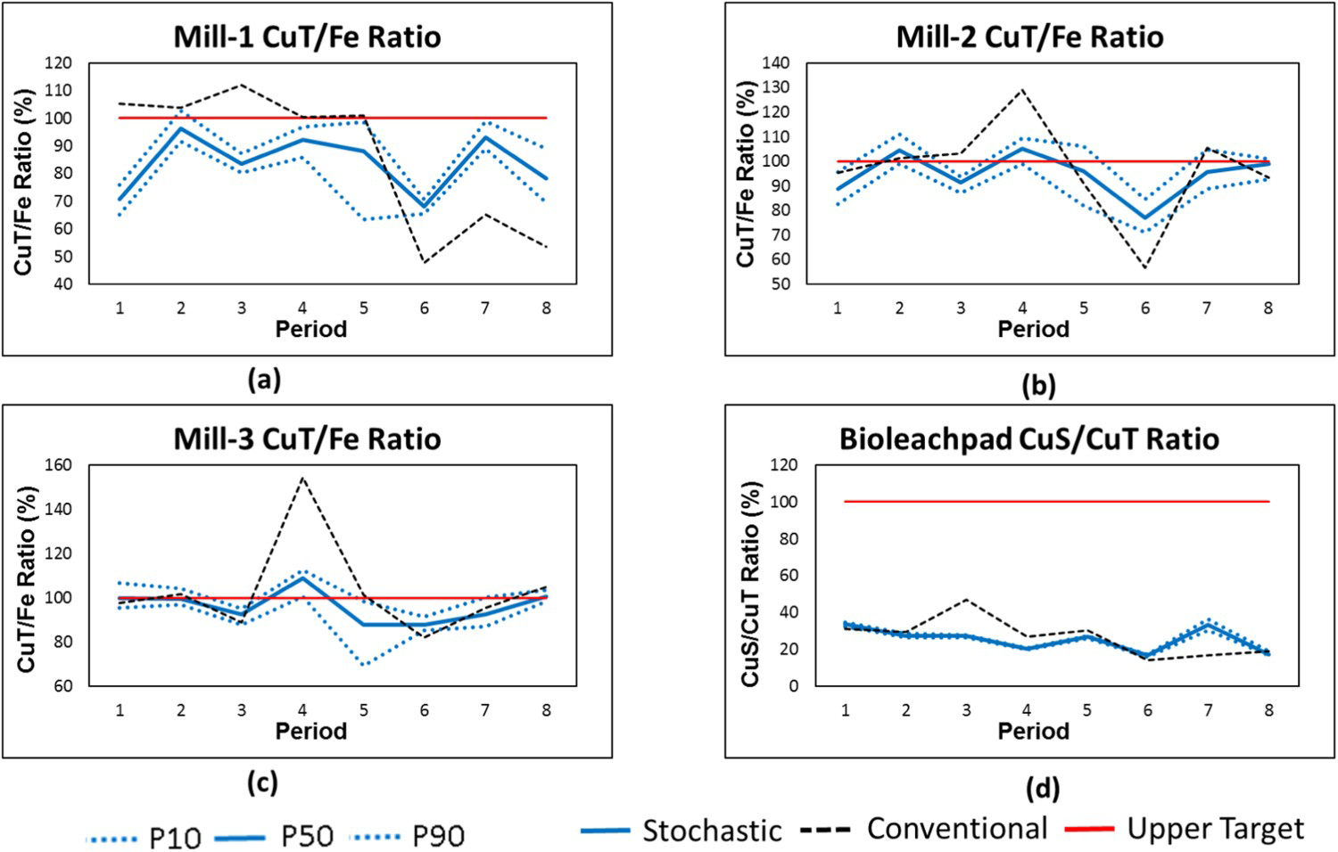
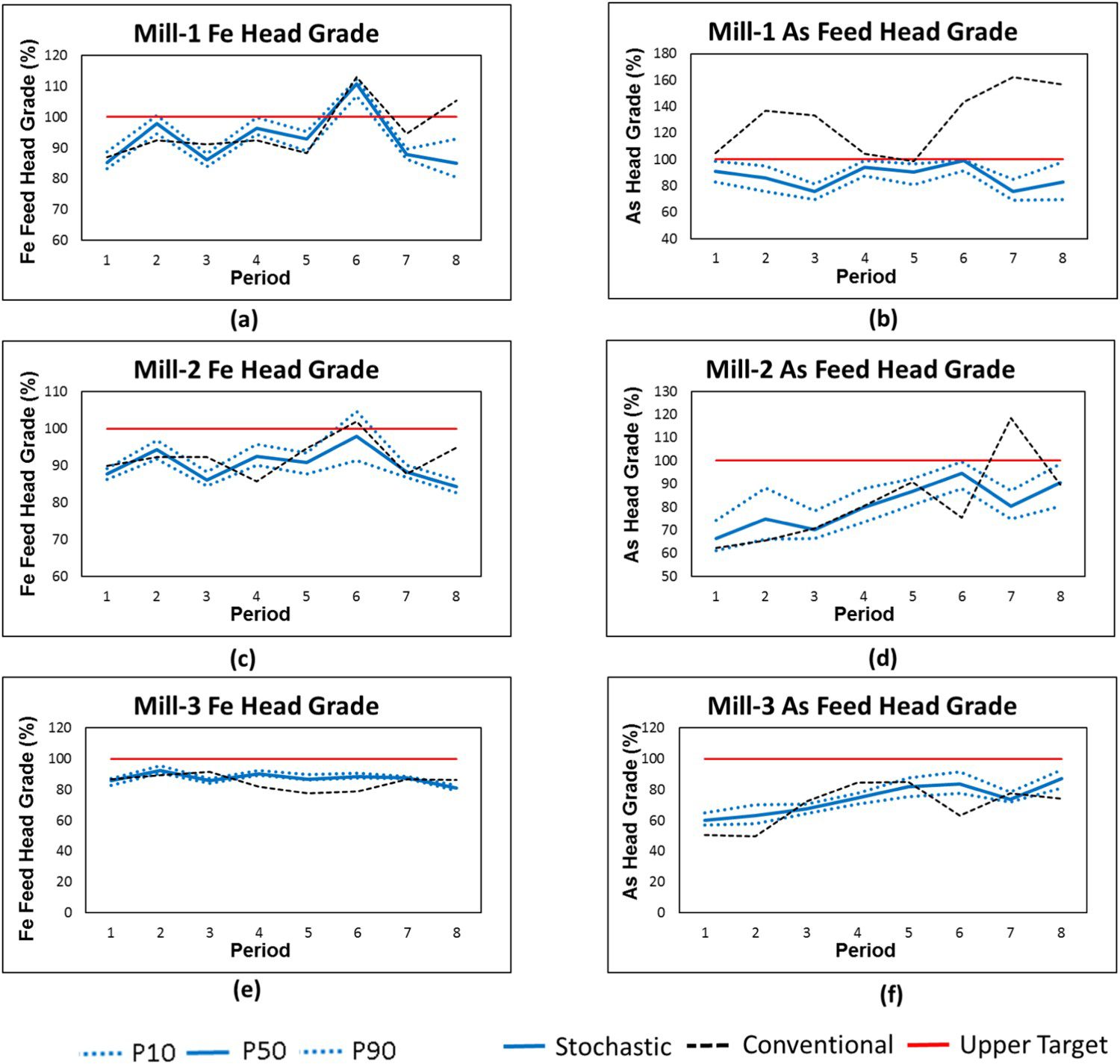
Figure 10(b,d,f) shows the risk profile of arsenic (As) head grade target for the different processing mills. The stochastic plan respects the arsenic head grade target very well for mill 1 (Figure 10(b)), mill 2 (Figure 10(d)), and mill 3 (Figure 10(f)). In the conventional plan, a large violation from the arsenic head grade target is expected over the scheduling period, particularly in year 2, 3, 6, 7, and 8 for mill 1 (Figure 10(b)). Similar behaviour is observed for mill 2 arsenic grade target (Figure 10(d)), with a small violation in initial years and a larger one in later years. The arsenic target is well respected in the stochastic and conventional plan for the mill 3 (Figure 10(f)).
Geometallurgical targets
Figure 11(a,b,c) displays the risk profiles of geometallurgical targets (hard/soft material ratios) for mill1, mill 2, and mill 3. The stochastic plan presents a very small violation from geometallurgical targets only for mill 1 as compared to the conventional plan, which presents a very large violation from such targets for mill 1 and mill 2 (Figure 11(a,b) respectively). The conventional plan does not account for geometallurgical properties in the optimization model but only uses it for determining processing stream utilization decisions. The geometallurgical targets are well respected for mill 3 for stochastic and conventional plan (Figure 11(c)). In addition, the stochastic plan shows stable geometallurgical target forecasts with significantly less fluctuation over the scheduling period as compared to a higher fluctuation in the conventional plan. Maintaining such a stable proportion of hard and soft material helps to achieve better throughput rates and efficient planning of processing mill operations.
Forecasts of geometallurgical target for mill 1, 2, and 3 for the stochastic and conventional plan.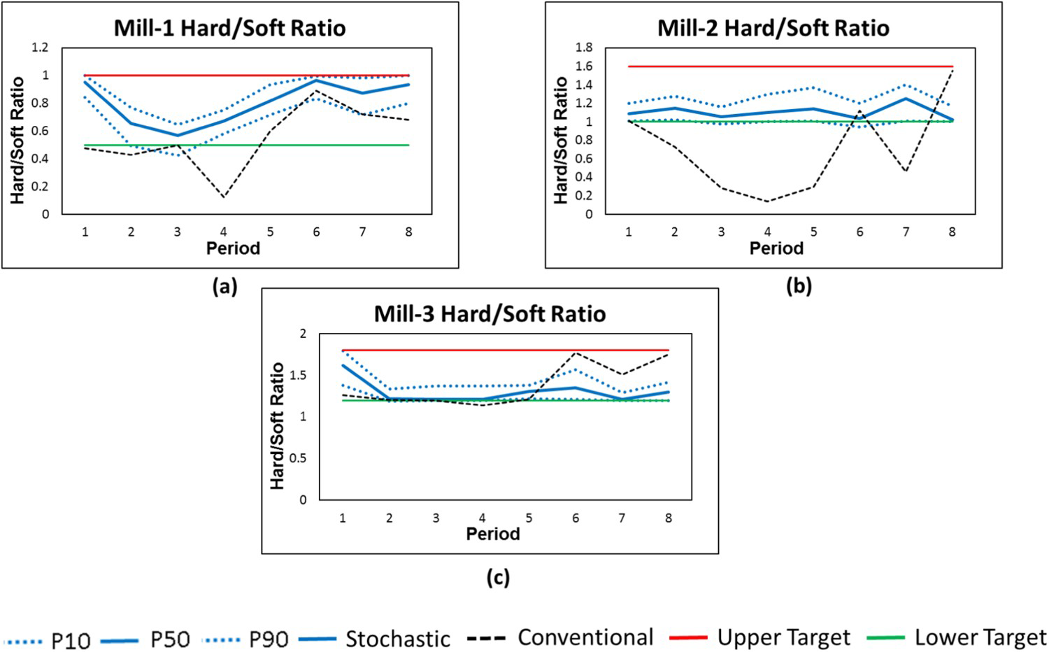
Metal production
Figure 12(a–d) shows the risk profiles of the recovered primary (copper concentrate) and secondary products (gold concentrate, silver concentrate, and molybdenum concentrate). The values are scaled with respect to the conventional plan (the conventional plan is 100%) for reasons of confidentiality. The stochastic plan produces 12.5% higher primary copper product (Figure 12(a)) as compared to the conventional plan over the scheduling period of 8 years. A higher production of secondary products, that is (i) 22.9% of gold (Figure 12(b)), (ii) 32.4% of silver (Figure 12(c)), and (iii) 34.7% of molybdenum (Figure 12(d)), is observed in the stochastic plan compared to the conventional plan. Such significant differences come from (i) capitalizing on synergies of simultaneous optimization of complete mining complex, (ii) capitalizing on the variability of material supply, and (iii) capitalizing on the added value of secondary products to drive the optimization process. Note, the conventional plan only considers copper in its production planning because the mining complex is a major producer of copper products and, therefore, does not account for other minor elements in planning decisions. As a result, the conventional plan is unable to capitalize on benefits generating from the added value of such secondary products to drive the optimization process. The secondary products are recovered as a by-product and, therefore, the value from such products were included in the forecast of conventional plan during comparison presented herein.
Forecasts of cumulative copper, gold, silver, and molybdenum recovered in the mining complex for the stochastic and conventional plan.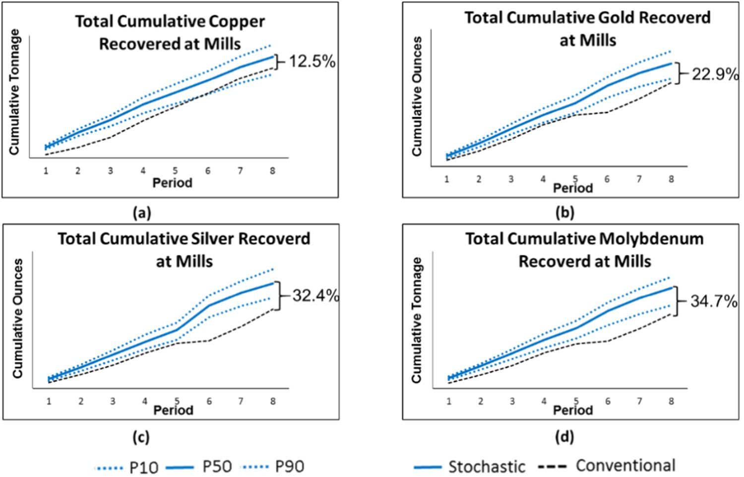
Discounted cash flows
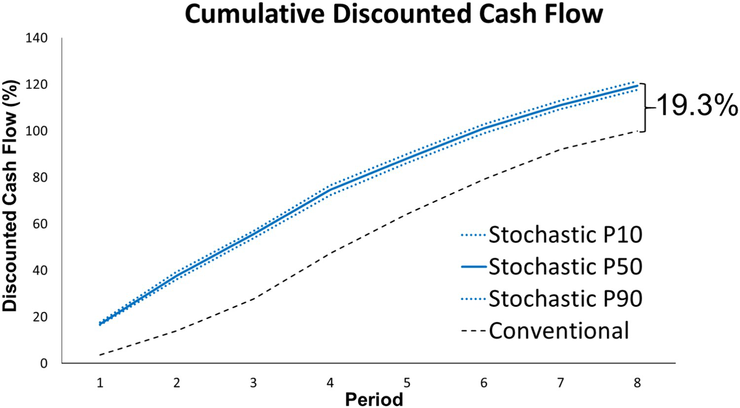
Figure 13 represents the risk profile for NPV forecasts. NPV is the cumulative discounted cash flow. The values are scaled with respect to the forecast of the conventional plan (the conventional plan is 100%) for reasons of confidentiality. The stochastic plan presents a 19.3% higher NPV compared to the conventional plan, for several compounding reasons. The large difference in the NPV forecast of the stochastic plan compared to the forecasts of the conventional plan is due to:
The ability to capitalize on synergies between the different components of the mining complex by jointly developing the extraction sequence, destination policies, and processing stream utilization under grade, geometallurgical and material type uncertainty, to maximize the value of products sold to the different customers. Incorporating uncertainty and variability of grade, material type and geometallurgical properties of the material in the stochastic optimization model helps to manage the technical risk throughout the life of mining complex and increases the expectation of meeting the different production target, including major effects on blending, destination policies, and processing stream utilization. Integration of different blending and capacity restriction in the simultaneous stochastic optimization model allows for better utilization of processing mills and crusher through the blending of material from multiple mines (as observed in Figure 7). The conventional plan, on the other hand, optimizes extraction sequence for multiple mines independently and, then, uses a separate optimization model to define processing stream utilization decisions to satisfy blending restrictions. Two-step optimization leads to underutilization of processing mills and crushers to meet the blending restriction. The ability to focus on the value of product sold rather than the economic value of the mining blocks. The utilization of secondary products such as gold, silver, and molybdenum in the optimization process of the long-term stochastic mine plan (as observed in Figure 12).
Cumulative discounted cash flow forecasts for the stochastic and conventional plan.
Production schedule
Figure 14 displays the cross-sectional and top view of the extraction sequence of the copper–gold mining complex. The smoothing constraints implemented with the model help to generate mineable shapes for the extraction sequence in the stochastic plan. The stochastic plan, extract material in different proportions form the multiple mines compared to the conventional plan to meet the required production targets. In addition, the stochastic and conventional schedule is physically different with different areas being mined in different years in the two schedules.
Generated schedule (a) top view mine A, (b) cross-section view mine A, (c) top view mine B, (d) cross-section view mine B; for the stochastic and conventional plan.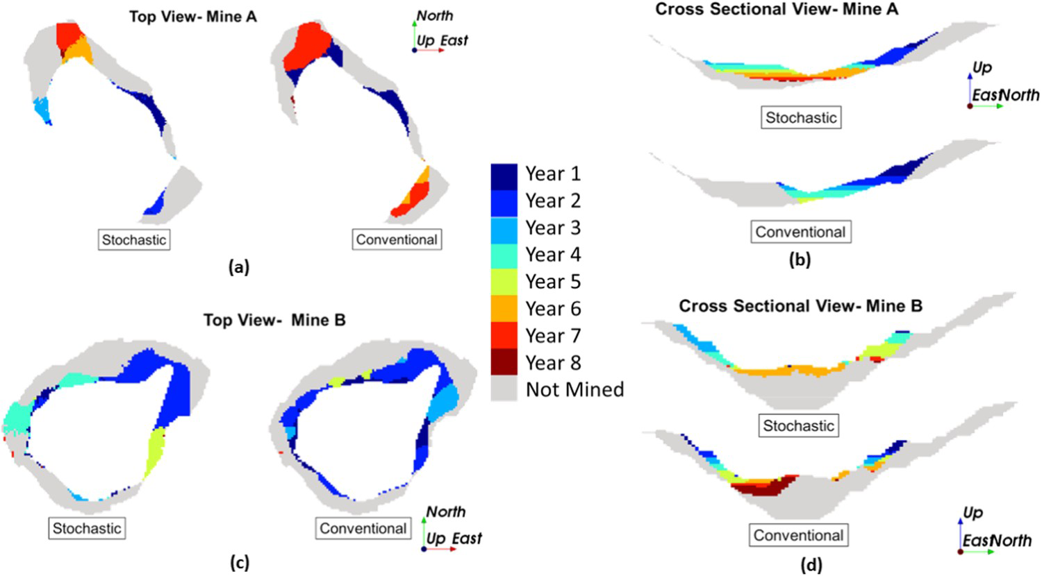
Conclusions
The simultaneous stochastic optimization of mining complexes is revisited and extended to include geometallurgical uncertainty and decisions. The model presented herein is very flexible and can be applied at any mining complex with different geometallurgical properties, production characteristics and constraints. The parameters of the stochastic optimization model presented require some trial and error in generating mine plans that maximize NPV, similarly to any other optimization method for strategic mine planning. The contribution and applied aspects of the proposed approach are highlighted with an application at a large copper–gold mining complex that consists of 2 mines, 5 crushers, 2 stockpiles, 3 processing mills, 1 waste dump and 2 leach pads and produces copper, gold, silver and molybdenum products for different customers and spot market. Two geometallurgical properties related to grindability of the material, SPI and BWI are considered in the optimization model, which increases the utilization of different processing mills in the mining complex. The forecasts of stochastic mine production plan show increased expectation of meeting the different production targets, including consistency in throughput and hardness of material processed at the processing mills and crushers, when compared with the forecasts of the conventional mine production plan. In addition, the stochastic mine production shows 12.5% higher production of copper metal compared to the forecasts of the conventional mine production plan.
The utilization of secondary products in the stochastic optimization model increases the forecasts of production of gold, silver, and molybdenum by 22.9, 32.4, and 34.7% compared to forecasts of the conventional mine production plan. The stochastic mine production plan also improves the NPV of the mining complex by 19.3% compared to the conventional mine production plan. Future work can consider integrating the decisions about operating modes such as coarse, medium, and fine grinding of material in the optimization model. Incorporating such operating modes decisions in the optimization model will help to enhance the performance of comminution circuits by choosing different operating modes based on the hardness of the material. Future directions also aim at integrating more geometallurgical properties in the optimization model. The results from the case study indicate that the available facilities (crushers, processing mills, leach pads, etc.) may be better utilized, providing further opportunities for value improvement through the inclusion of capital expenditure decisions in the simultaneous stochastic optimization model.
Disclosure statement
No potential conflict of interest was reported by the authors.