
Abstract
Power-Law topology has been proved to be an effective technique to improve fault tolerance. With the motivation of construct reliable topology for wireless sensor networks, a Power-Law Evolving Model (PLEW) of wireless sensor networks by stochastic placement is proposed in this article. In a dynamic evolving process of Wireless Sensor Networks, there are four types of events as follows: adding new nodes, nodes failure, adding new links, and links failure. The dynamics of nodes and links are integrated into the evolving model consequently. By using the continuum theory, the theoretical computing and simulated results show that the degree distribution of this model follows a power law. The scale-free properties revealed in this model can be applied into the scenarios required high dependability, such as national defense or survivability systems.
Introduction
Recent advances in nanotechnology have made it possible to develop a large variety of low power devices that integrate sensing, special purpose computing, and wireless communications capabilities. A Wireless Sensor Networks (WSNs) is a collection of many small devices, each with sensing, computation, and communication capability. It has many potential applications, such as building surveillance, environmental monitoring, etc.
The sensor node placement in wireless sensor networks can be divided into deterministic and stochastic placement [1]. The deterministic placement requires that each sensor node be placed at predetermined coordinates, while in stochastic placement, the positions of the sensor nodes are determined by a probability density function (p.d.f.). In the latter placement, approximate positioning satisfies the probability density function, which causes low placement cost. Due to node failure and limited node power capacity, the nodes placement turns out to be extraordinarily important, and stochastic placement has been testified to be an effective fault tolerance technique in [1]. Also, the forms of stochastic placement can produce scale-free properties, where the degree of the nodes follows a power law.
In this article, we consider a complex wireless sensor network by stochastic placement based on [1]. By analyzing the dynamics of wireless sensor networks, a Power-Law Evolving Model (PLEW) is proposed, where the degree distribution shows scale-free properties. The rest of the article is organized as follows. In Section 2 we basically describe related work and our contribution. In Section 3 we introduce a classical BA scale-free model. In Section 4, the design of PLEW is discussed in detail. In Section 5 we conduct the theoretical analysis by using the continuum theory, as well as the simulation, followed by the conclusions in Section 6.
Related Work and our Contribution
In the past few years, more and more researchers have devoted their enthusiastic energy to explore and characterize the evolving mechanisms of complex natural network systems, such as the Internet [2, 3], the World Wide Web (WWW) [4], traffic networks [5], food webs [6], etc. Empirical research by using the statistical approach shows that these networks generally exhibit universal properties of complex networks, including small-world characteristic [7] and scale-free characteristic [8].
Due to the limit of the wireless transmission range, wireless sensor networks belong to spatial graphs, and not to rational graphs [9]. Whether wireless sensor networks have the characteristics like other complex natural network systems, such as the Internet or the World Wide Web? What are small-world effects and scale-free properties in wireless sensor networks, including the degree distribution, the path length, and clustering coefficient? How to model the dynamics of wireless sensor networks? In 2002, Jin and Symeon et al. [10] modeled mobile wireless sensor networks, which described the dynamics of the network and facilitated the understanding of the effect of the various events, and this is the original work, to the best of our knowledge. In 2003, Mika et al. [1] probed the scale-free properties of wireless sensor networks by using the probability density function; she has proved that the power-law placement can constitute good placement with a well-tuned control parameter. Helmy [9] investigated the small-world effects in wireless networks by randomly link re-wiring and link addition. In 2004, Sarshar et al. [11] first showed that only relying on the classical BA model cannot produce heavy-tailed degree distribution in complex ad hoc networks and P2P networks. He has proposed an evolving model which introduced the mechanisms of nodes deletion and links compensatory rewiring; Saffre et al. [12] successfully implemented the scale-free topology for pervasive networks, which conquered the difficulty by devising realistic connection protocols that would allow approximating scale-free topology on the sole basis of local information exchange. In 2005, Chen GuanRong modeled the complex Internet topology in his preeminent work [3], which captured the Local-World evolving dynamics. In 2007, Qin et al. [13] proposed a complex ad hoc network model with accelerated growth based on [11] and [14]; Wang et al. [15] designed a topology control algorithm, which introduced the scale-free properties into the topology of Wireless Sensor Networks to minimize transmission delay and increase robustness; Garbnato et al. [16] investigated the impact of scale-free topologies on Gossiping in the context of Wireless Sensor Networks; Chen Lijun et al. [17] presented an evolving model with equivalent growth of the nodes, which was based on the BA evolving model [8] and Local-World evolving model [18], and this model can improve the uniformity of the degree distribution; Brooks et al. [19] used Bernoulli probability matrices to analyze the random graphs model of mobile sensor networks, which presented an application for the security of sensor networks.
Due to unforeseen reasons, the topology of WSNs often changes. How to model the dynamics of topology is very meaningful for constructing reliable WSNs, improving fault tolerance, and the efficiency of routing. Actually, in real networks, there are five types of evolving events: adding new nodes, nodes failure, adding new links, links failure, and links re-wiring. We consider links re-wiring as the combination of adding new links and links failure, so we do not analyze links re-wiring in this article. However, in most works we have mentioned, they considered the issue of adding new nodes, adding new links, and links failure, except the work reported in [1] and [11]. In this article, we specially consider the nodes failure or randomly attack in WSNs, and use the continuum theory [8] and the similar method in [3, 11] to predict the exponent of degree distribution; then we conduct the simulation to verify the validity of our model.
BA Scale-Free Model [8]
Evolving Process
The evolving process of the classical BA scale-free model includes two ingredients as follows: equivalent growth of the nodes and the degree of preferential attachment. The equivalent growth implies that the dimension of the entire network grows continuously, is different from the small-world network and random network where the number of nodes is static; the degree of preferential attachment means adding new nodes incline to be attached with high-degree nodes. Based on the two aspects which have been mentioned, the evolving process of the BA model is carried out as follows:
Equivalent Growth
Starting with m0 nodes, at every time step t we add a new node with m links that connect the new node to m different nodes already present in the network (m < m0).
Preferential Attachment
The probability π
i
that a new node will be connected to node i depends on the degree ki of that node, so that
Analysis of Degree Distribution
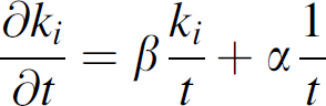
In the BA model [8], the continuum theory was used to analyze the degree distribution. The rate at which a node acquires links is:

Power Law Evolving Model by Stochastic Node Placement
Network Formalization Definition
In general, the nodes of WSNs are placed in a coordination in 2-D or 3-D euclidean space and the entire sensor network is formalized as a unit disk graph G = <V(G),E(G)>, where V(G) = {v1, v2, …,v3} is the set of nodes and E(G) the set of wireless links; rangevi is the max transmission range of sensor node vi [20]. If the distance between vi and vj is less than rangevi, link(vi, vj) will exist. In real sensor networks, the transmission range of each node may not be a perfect disk. In this case, the network is a quasi-unit disk graph. Thus E(G) can be expressed as:
Network Parameters
The degree of nodes can describe the importance of nodes in the network. We define p(k) as the probability of the nodes which have k degree. A different network has a different p(k) function.
The network distance and diameter of the network can not make overall evaluation. We need to introduce the average path length. The graph G = <V(G),E(G)< is usually described by means of two parameters: the average path length L and the clustering coefficient C. The average path length L is defined as the minimum distance between any pair of nodes (i,j), averaged over all possible pairs, and showed as follows:
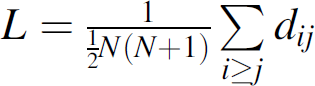
Considering the situation of non-connected graph, we define L as follows:

The clustering coefficient describes the aggregation level of the network, and the clustering coefficient Ci of node i is defined as the actual edges exist in the ki neighbors of nodes i divided by the edges while neighbors are fully connected, and
Algorithm Design
The initial network has m0 nodes and e0 edges with the same condition of the BA model. Nodes will be placed in L × L square area, the coordinate of nodes will be decided by p.d.f. The transmission range of the sensor node is R. The algorithm will produce N nodes. At every time step t, perform one of the following phases at random:
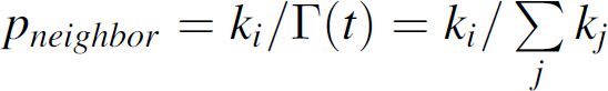
With probability p1, a new sensor node is placed into existing networks, which has m1 links to the neighbor nodes of existing networks (Fig. 1). The preferential attachment probability
And the sink node (base station) should broadcast HELLO message to all the nodes. We define three types of messages as follows:
HELLO message CONNECT message CONFIRM message The type field is specified as 0 to 7, which means sink HELLO message of adding new node, sink HELLO message of adding new links, sink HELLO message of node failure, sink HELLO message of links failure, HELLO message of common node, CONNECT message, and CONFIRM message respectively. The node whose ID is SelectedID will set the SelectedFlag and AlivedFlag field to 1, and broadcast HELLO message to its neighbor nodes, then select the m1 nodes, send CONNECT message to the m1 nodes, and the nodes send CONFIRM message back to the SelectedID node. This is the procedure for establishing the m1 links. With probability p2, m2 links is added into existing networks (Fig. 2). The sink node randomly selects one node whose ID is SelectedID, the node will select one neighbor node with pneighbor to establish one connection. This procedure is performed with m2 times. With probability p3, the event of one node failure will happen (Fig. 3). The sink node randomly selects one node whose ID is SelectedID. The node will set the SelectedFlag and the AlivedFlag field to 0, and disconnect with its neighbor nodes. With probability p4, the event of m3 links failure will happen (Fig. 4). The sink node randomly selects one node whose ID is SelectedID, the node will disconnect with its neighbor nodes. This procedure is performed with m3 times.


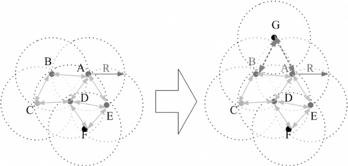
Adding new node with probability p1.

Adding new links with probability p2.
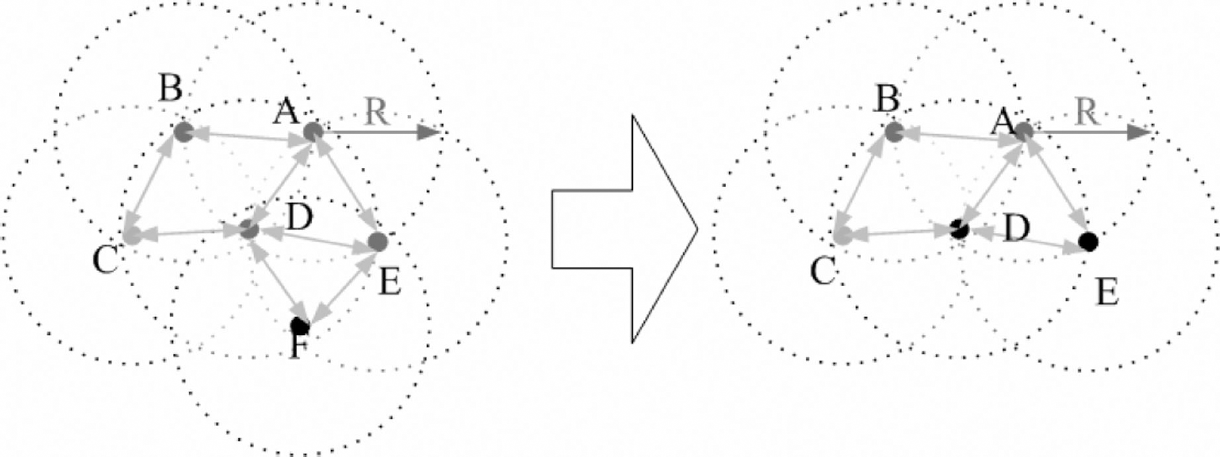
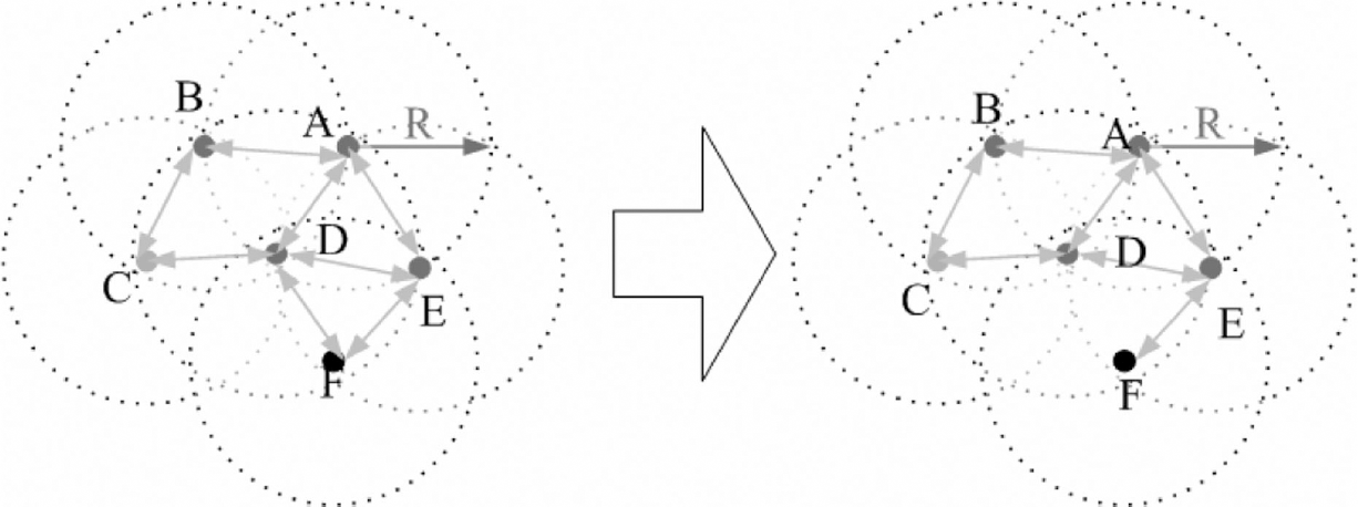
Node failure with probability p3.
Links failure with probability p4.
The flowchart of the algorithm is the following:
In order to verify the validity of this model, we conduct the theoretic analysis, and then develop MATLAB toolbox for simulation, as well as we compare the theoretic analysis and the simulation results.
Theoretic Analysis
We define some analysis parameters as follows:
At time t, the total number of nodes:


From evolving rule (1), we can get the dynamic equations of ki

From evolving rule (2) and the similar method in [3], we can get the dynamic equations of k i

From evolving rule (3) and the similar method in [11], we can get the dynamic equations of k i

From evolving rule 4 and the similar method in [3], we can get the dynamic equations of k i

The summary of analysis parameters

By combining Eqs. (5–8), the total dynamic equations of ki is as follows:

With the condition of t − >∞,

Then
Taking into account the initial condition ki(ti) = m1, the solution of Eq. (11) is:

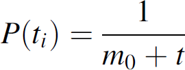
Assuming that we add the node into the networks at equal time intervals, we obtain the probability density function of time ti:
Therefore,

Then we get the probability density

Over long time steps, the Eq. (15) will lead to stationary solution as follows:
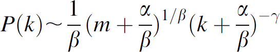
In the case of
We develop a MATLAB simulation toolbox for verifying the validity of this model. Randomly distributed nodes are placed within a two-dimensional network space which is set to 1000 m × 1000 m. The sink node or base station is placed at (0, 0). The transmission range is respectively set to 20 m, 30 m, 40 m, 50 m, 60 m, 70 m, 80 m, 90 m, 100 m, and 110 m. We start our simulations under four different situations:
Figure 6 shows the degree distribution of our model, which exhibits a power law, and Fig. 7 shows the exponent of degree distribution with different situations. Note that the degree exponent of simulation is a little different than the predicted value, that is caused by randomly links failure. Figure 8 shows the average degree of our model and especially the probability of nodes failure has an important impact on the results. Figure 9 shows the clustering coefficient of all simulations. Figure 10 shows the average path length, with the same reason of Fig. 8, the average path length is much higher than the theoretical value. Figure 11 shows the diameter of the model. From Figs. 10 and 11, we come to know that the probability of nodes failure can affect the network topology, and the higher the probability is, the more the nodes will fail, then either the path length or the diameter will increase consequently. However, this model is robust with randomly nodes failure and links failure. Based on Figs. 6 to 11, the simulation results are in agreement with our theoretical analysis.

Flowchart of the algorithm.

The degree distribution.
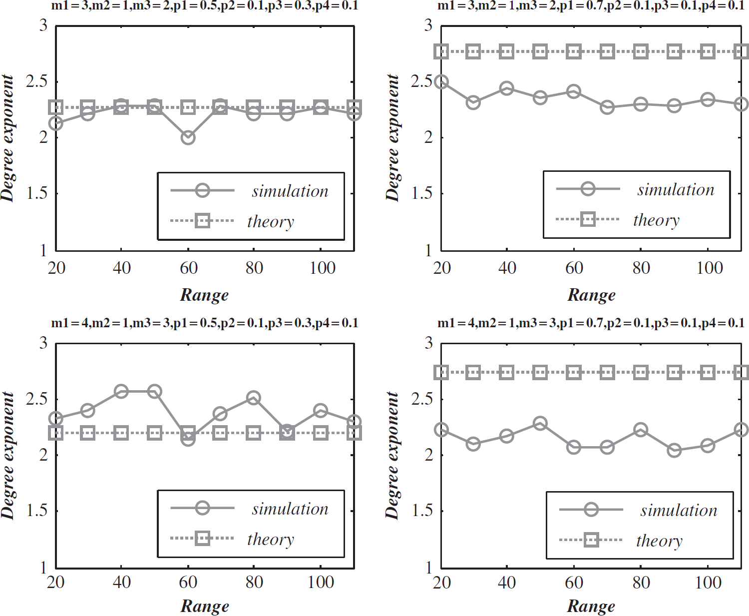
The degree exponent with different situations.

Average degree with different situations.
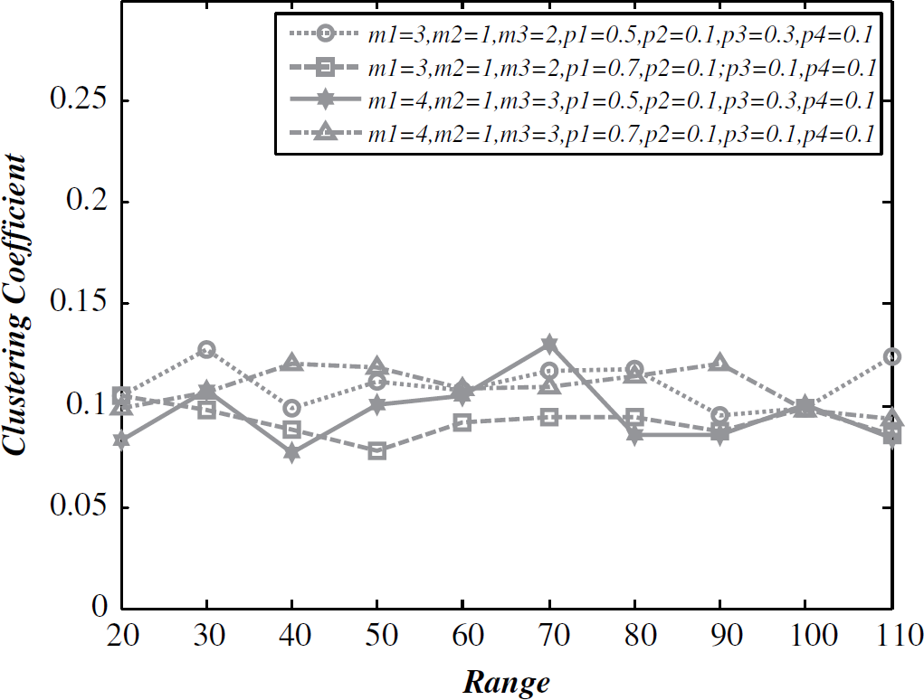
The clustering coefficient.

The average path length.

The diameter.
In many schemes of topology control, the sensor nodes are evenly placed in the space, and the nodes are not clustered, such as in [20]; on the other hand, the nodes may form the cluster with specific protocol, such as LEACH [22]. Our motivation and potential applications in this article have come from our research of national defense, which need to construct reliable wireless sensor networks. The sensor nodes are densely placed in a hostile region, and even a small part of the nodes are destroyed by hostile staff, the power-law topology will constitute better performance following the above analysis. The similar applications can be found in [1, 15, 19].
In this article, the dynamic evolving topology of wireless sensor networks has been modeled. The following evolving events are introduced into the evolving model: adding new nodes, nodes failure, adding new links, and links failure. We use the continuum theory to predict theoretically the exponent of degree distribution, and the analysis results shows that our model exhibits scale-free properties, and the degree distribution exponent is between 2 to 3 with appropriate parameters. In the situation of randomly node failure and links failure, this model has higher robustness, which provides a reference for constructing reliable topology of Wireless Sensor Networks. In future work, we will focus on improving robustness and introduce weighted networks to further enrich this model.