Sage Journals: Discover world-class research

Abstract

The multi-modal tracking model in [1] enables the on-the-fly error compensation with low complexity by adopting acoustic sensors for the main tracking task and visual sensors for correcting possible tracking errors. The visual compensation process in the model is indispensable to the accurate tracking task in a dynamic object movement.

This article proposes an algorithm to approximate the successful visual compensation rate appearing in the multi-modal tracking system. The acoustic sampling interval of the object signal and the random occurrence of transmission delays of multi-modal data are critical to the compensation process. Therefore, by using the two key factors as parameters, the algorithm called SEA can estimate the successful visual compensation of a tracking system. After we build up a tracking system, it is required to maintain the system at a certain level of tracking accuracy. This task can be done by controlling the aforementioned parameters since the visual compensation influences the tracking accuracy. Thus, we propose another algorithm called SEA² for the parameter adaptation. The algorithm controls only acoustic sampling interval due to the easiness of adjustment and having the main impact on the success of the visual compensation. From the algorithm validation, we show the SEA properly quantifies the visual compensation process successfully occurring in the tracking scenarios, and SEA² is feasible for parameter adaptation and achieving the target level of accuracy.

Keywords

Multi-Modal Sensor Tracking System Visual Compensation Statistical Estimation and Adaptation

1. Introduction

A tracking system is used in diverse areas like mining, military, and hospital. However, it is difficult to achieve reliable and robust tracking results since the unpredictable trajectory and diversified environmental errors exist. For the tracking task, acoustic sensors have been widely used in many applications due to the advantages such as the low cost of deployment and flexibility. However, they are not only sensitive to a reverberant indoor environment which frequently generates extraordinary signals, but also having difficulty in satisfying the requirement of consistent data. Thus, other types of sensors to assist the acoustic operation are necessary to obtain more reliable data. Among a variety of sensors, a visual sensor can be a good candidate to collect consistent and reliable data. In this multi-modal tracking environment, the audio-video joint processing provides more accurate data by mutually complementing the errors appearing in the middle of tracking.

The authors in [2] have proposed Particle Filter (PF) [3–6] based tracking architecture for the multi-modal sensor fusion to track people in a video-conference application. They use the audio signal for a complementary data to video measurement, and increase the tracking accuracy by merging the audio and vision measurement. However, since the video image processing requires high processing complexity, the joint measuring method could not lead to the expected tracking accuracy in a real-timing environment with high volume of images.

The tracking model in [1,7] has a different type of modality for the tracking task. It uses acoustic sensors to mainly track the objects and visual sensors to compensate the tracking errors. It has the advantage such as the on-the-fly error correction with low computing complexity. Moreover, the tracking framework is applicable to not only open space where line-of-sight (LOS) is guaranteed, but also blocking space where LOS is not perfectly guaranteed by moving obstacles like trees in the outdoor environment and high loaded carts in the indoor circumstance. In this situation, the acoustic signals that turn over the obstacle and arrive at the acoustic sensors are good measuring data for the tracking task. However, acoustic-based tracking can be deviated from a real object trajectory as the environment generates a noise that creates distortion to the normal signal. In this case, the visual sensors correct the tracking errors of the acoustic sensors.

When an acoustic sensor with adjacent microphones is sampling an object signal, the PF algorithm associated with the acoustic sensor obtains the object coordinates. A visual sensor supports the tracking task by correcting the PF estimation error based on the localization algorithm with a parallel projection model. Since the processing overhead of PF is a few microseconds [8] and the localization algorithm for visual compensation is rarely performed compared with the PF calculation, the tracking model can minimize the overall processing overhead. In the tracking system, a processing server collects the multi-modal data and performs a localization algorithm, and routers relay the sensor data. To represent the success or fail of a visual compensation by a numeric value, the authors have defined a new performance metric, Successful Compensate Rate (SCR) which is applicable to the tracking system. The SCR is the ratio of the number of PF-error correction assisted by visual sensors over the total number of PF-estimate generation from acoustic sampling. The SCR has a role in gauging the accuracy of the tracking task.

The motivation of this paper is to quantify the tracking accuracy and the behavior of the tracking model in [1,7] by constructing a numerical model to estimate the SCR. By the analysis model, we can accelerate the system evaluation before establishing a real tracking system. To do this work, this paper proposes an algorithm, Statistical SCR Estimation Algorithm (SEA), to approximate the number of success to appear in the multi-modal system with acoustic sensor for main tracking. The success of visual compensation depends on the acoustic sensor's interval to sample the object signal, and the transmission delays of sensor data between multiple sensors and a server. Especially, we cannot predict the size of delays since a tracking network has a number of delay factors like router capacity and background traffic volume. Thus, the transmission delay has a randomness property. Based on this aspect, the SEA approximates the SCR by using the two key factors as the algorithm parameters.

For the algorithm formulation, we first observe the transmission delay between the multi-modal sensors and the server. The observation results reveal that the delay from visual sensors to the server is modeled by Gaussian Probability Density Function (PDF), and a delay from the server to the acoustic sensor follows Exponential PDF. From the PDFs, the SEA generates random values to imitate the delay in a real situation. Then, it uses the random values and pre-determined acoustic sampling interval as parameters, and determines the next status according to transition rules that have four modes (R, L, B, and U) and two states (s and f). The transition rules have restrictions that only state-to-mode transition is allowed and there are no mode-to-mode, state-to-state, and mode-to-state transitions.

After establishing a tracking system, it is necessary to maintain the system at a given level of tracking accuracy. This objective can be achieved by controlling the acoustic sampling interval or the transmission delays since the tracking accuracy depends on the SCR of visual compensation. Thus, we propose another algorithm, Statistical and Estimation and Adaptation Algorithm (SEA²). The algorithm controls the acoustic sampling interval to adapt the level of tracking accuracy since the parameter is simple to adjust and mainly affects the success of the visual compensation. In the parameter adjustment, SEA² uses the SEA algorithm to obtain an initial sampling interval ( $Δ t_{s}^{0}$ ) and consists of Phase 1 and Phase 2. Since the SEA requires the mean and standard deviation for the PDFs, Phase 1 performs the estimation of the population parameters. Based on the estimation, the SEA is executed to obtain $Δ t_{s}^{0}$ . In Phase 2, the algorithm uses exponential increase or decrease of $Δ t_{s}^{0}$ to reach fast the target tracking accuracy level.

The validation of both algorithms is performed by NS-2 [9] simulations by constructing string and tree scenarios. In the validation of the SEA, we observe the achieved SCR(%) in various acoustic sampling intervals. The results indicate that low SCRs are achieved when acoustic sensors are far from the server, the sampling interval is short, and the image size is small. We verify the algorithmic accuracy of the SEA by showing that the mathematical calculation in the SEA properly approximates the simulated SCR results. For SEA² validation, we observe how the SEA² automatically adjusts acoustic sensors' sampling interval to achieve a target SCR. The simulation results show the sampling interval adjustment is well performed when we set up the target SCR to 90%. In order to observe the real-timing adaptation capability of the SEA², we change the target SCR in the simulations from 30% to 60 and 90%. The results indicate SEA² also has a confidential adjustment mechanism in the real-timing case.

Organization of this article is as follows. In Section 2, we explain the background information and the motivation of this paper. The details of the SEA are illustrated in Section 3, and the SEA² is explained in Section 4. The algorithm validation is performed in Section 5. Finally, we conclude in Section 6.

2. Background and Motivation

2.1. Tracking by Multi-modal Sensors

An acoustic sensor is widely used for the tracking task since it allows easy and quick deployment with less computational complexity as well as broad sampling range. The Particle Filter (PF) algorithm [6] associated with the acoustic sensor mainly generates the coordinate estimate of a moving object even with non-linear model and non-Gaussian noise. PF is a powerful method for sequential signal processing for nonlinear and non-Gaussian problems. It is broadly used in applications that need the tracking and detection of random signals. However, it has two key problems in performing a tracking task. The first problem takes place when the initial state is not clear or reliable. Since the PF algorithm assumes the initial state is clearly given, the PF approximation outputs show significant deviation from the real object trajectory in the presence of the initial state problem. Another problem is a trajectory divergence problem. In the middle of a tracking task, the tracking model could be dynamically changing. In this case, if the model is not correct at a point, the next PF estimate gradually deviates from the real object trajectory since the current PF state depends on the previous state. Continuing with the PF problems, the acoustic sensor equipped with the PF has the limitation such that it can not provide a consistent measurement if the target objects move without sound emination.

In order to overcome the problem of the acoustic sensors, an audio-visual multi-modal tracking algorithm [2] has been proposed to provide accurate and fast system implementation. However, the main tracking in the algorithm is performed by the visual sensor and assisting task is done by acoustic-based PF algorithm. In this case, the complexity of image processing can be a processing overhead in the tracking task.

2.2. Target Application Model

In order to solve the overhead problem in the audio-visual joint tracking system and the non-line-of-sight (NLOS) problem of the visual sensor, we have developed an application model for the tracking task [1, 7]. The tracking model takes the integration of an acoustic sensor and two visual sensors as shown in Fig. 1. A three-dimensional acoustic localizer obtains the direction of arrival (DOA) [10] at an acoustic sensor, and detects two angle components θ and ϕ from the arrival time difference between embedded adjacent microphones. Then, the object estimation errors are corrected by the association with two visual sensors. The tracking model solves the processing overhead problem since a low computational PF algorithm mainly tracks objects and visual image compensates the tracking error caused by the aforementioned key problems in the PF algorithm. Moreover, the tracking model is working even in the situation that the line-of-sight (LOS) of the visual sensor is not perfectly guaranteed by moving obstacles in a tracking space. In this situation, the acoustic sensor is a good device for sampling the object signal since the acoustic signals can diffract the obstacle and be captured by acoustic sensors. However, only acoustic sensor-based tracking can be deviated from real object movement as the tracking environment makes a noise. In this case, the visual sensors correct the tracking errors of the acoustic sensors.

Figure 1.

Target application model for object tracking. It consists of an acoustic sensor and two visual sensors to capture the object information.

In a visual compensation process, we use a localization algorithm based on parallel projection model [11] to obtain the object coordinate from the visual image. Here, the PF calculation is done at an acoustic sensor, and the visual compensation is performed at a server. We can construct the tracking system as a fully-distributed wireless system such that distributed routers perform the PF and localization algorithms. However, as we have indicated in [12], router-based architecture has large end-to-end transmission delay of the visual image since the visual sensors have to send the same image to all the routers. Note the image size from a visual sensor is relatively larger than that of the acoustic sensor even if the image size depends on camera types. For example, the IP camera [13] in our test generates visual images with 30 KBytes to 55 KBytes size. Therefore, the application model uses the server-based architecture to reduce the duplicate transmission of the same image as well as to use the high computational power and easy reconfigurability of the server system.

2.3. Visual Compensation Effect

Figure 2 shows how the tracking accuracy increases when the visual sensor assists the tracking task in the application model. In Fig. 2a and b, we track only one object, and Fig. 2c and d represent the estimation results when three objects are moving in the tracking space. In the simulations, we set up the visual sampling interval (Δt_u) which is 10 times larger than the sampling interval (Δt_s) of an acoustic sensor, and use 500 for one target object case and 200 particles for the three target objects case. The red line is the actual object path, and the blue line indicates the tracking estimate. In this spiral movement, we can understand that the tracking system should adopt the visual compensation process to obtain the accurate object tracking.

Figure 2.

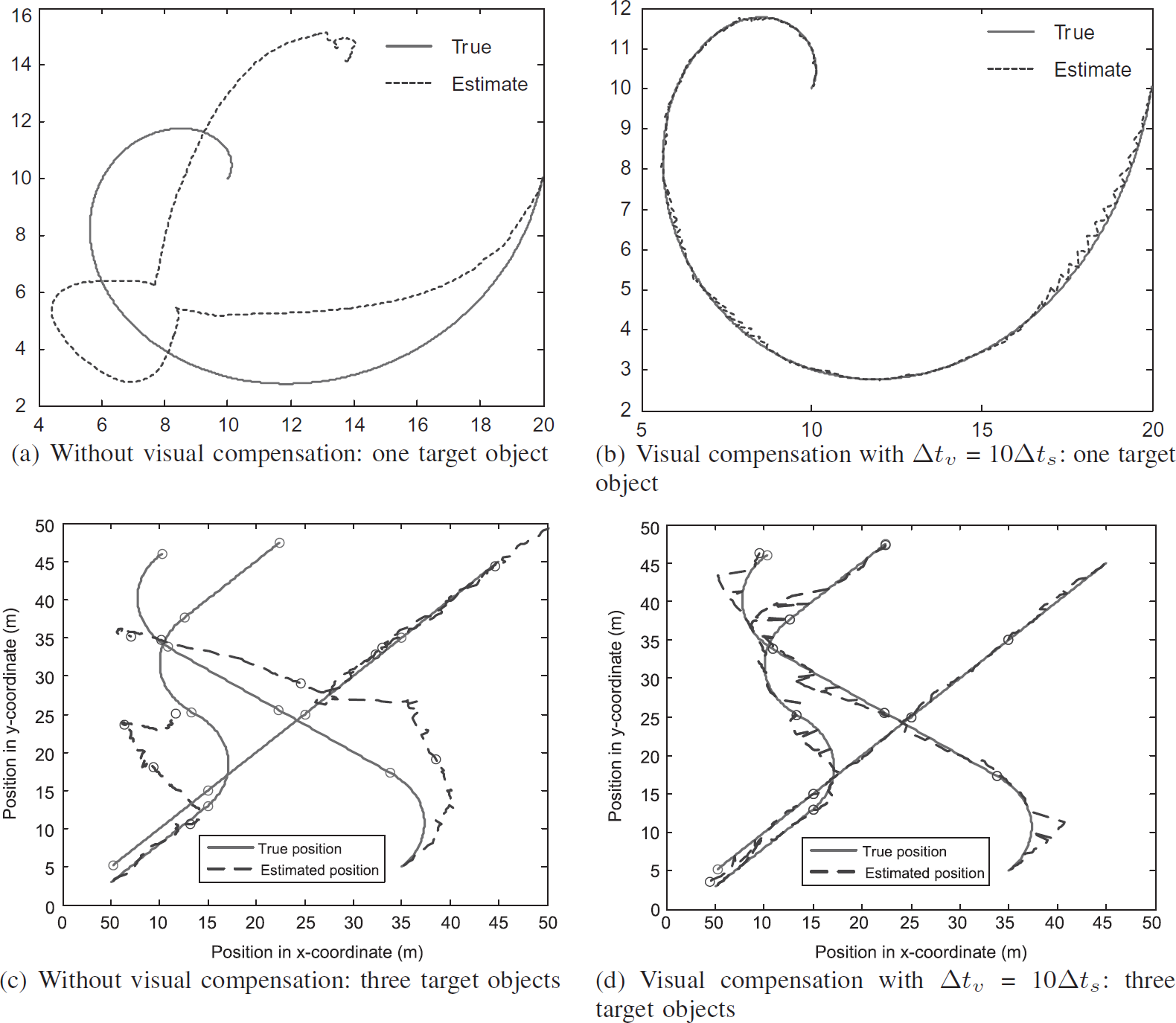
Effect of visual compensation in the tracking system. Here, we track one object. In the simulations, 500 particles are used in (a) and (b), and 200 particles are used in (c) and (d).

However, this significant improvement is based on the assumption that (1)

as soon as acoustic and visual sensors are sampling object information, the visual compensation process takes place without time delay, and

(2)

the visual compensation results are immediately applying to the next PF generation.

However, the sampling and the calculation points generally locate in different places, so that we need to identify a network synchronization problem caused by data transmission delay within a network.

Figure 1 represents the factors to be considered in the tracking model at the network point of view. An acoustic sensor receives the object signal at t_i while visual sensors 1 and 2 capture the image at time t_i+1 and t_i+2, respectively. After independently sampling the object information, each sensor sends the information to the server. The transmission delays from visual sensor 1 and 2 to the server are denoted by x^v1 and x^v2, and the delay to deliver PF estimation from the acoustic sensor to the server is represented by z. Additionally, the acoustic sensor requires feedback from the server to get the visual compensated object position for the adjustment of the next PF calculation, which takes y transmission delay. We define the tracking problem caused by the network transmission delay in visual compensation process as a network synchronization problem. The independent data transmission delay in addition to sampling time difference among multiple sensors causes the network synchronization problem. We have proposed a solution for this problem in [7].

2.4. Definition of Success and Fail Conditions

The x^v1, x^v2, y, and z in the previous section take random values in real situations according to the status of a tracking network. Due to the randomness property, we cannot predict when the multiple sensor data arrive at the server for visual compensation calculation and the feedback reaches the acoustic sensor. Due to this phenomenon, the server could have no image frames, or have enough number of images at the point of execution of a visual localization algorithm. In this case, the server has to determine whether it performs the localization algorithm, and if it can execute the algorithm, which one among the already received images is the best for the algorithm execution. Moreover, if visual sensor 1 captures the tracking space too much earlier than the other visual sensor and its capturing point is also too early compared with the acoustic sampling time, the image from visual sensor 1 can not give the correct information in the visual compensation process even if the server receives enough number of image data for the algorithm execution. Therefore, to clearly define when the visual localization algorithm can be running and what is the success of the visual compensation, we make two conditions as follows.

Condition 1: The server sees that the sampling times of both visual sensors are later than the acoustic sampling time of previously arrived acoustic data. At this point, the server performs the localization algorithm.

Condition 2: The compensated estimate should be feedbacked to acoustic sensors before the next acoustic sampling time.

If the above conditions are satisfied at the same time, we define this case as success. We regard other cases not satisfying the above conditions as fail even if it actually does not mean the failure of the algorithm calculation.

Figure 3 shows the message flowing diagram between the sensors, the router, and the server, and possible success and fail cases in the tracking model. In the figure, the messages related with acoustic sensors are directly delivered from the source to the destination by using the UDP protocol, and the visual image that needs reliability is delivered by TCP. Since the visual image size is larger than the Maximum Transmission Unit (MTU) size, more than one packet is exchanged between the visual sensors and a server. The acoustic sampling times are denoted by red arrows and the blue arrows are for visual image capturing points. We additionally add red points to represent the calculation of the localization algorithm at the server side. We can understand only Fig. 3a satisfies both Conditions. Note in Fig. 3c and d, the final result is not success due to the network synchronization problem even if the localization algorithm is successfully executed.

Figure 3.

An example of success and fail cases in the tracking model.

2.5. Impact of Network Synchronization

In this section, we investigate the impact of the network synchronization problem by simulation study. We use the same simulation scenario as Fig. 9a where 15 acoustic sensors conduct the sampling for each ranging area, and two visual sensors capture the tracking space. The multi-modal sensors send the sensing data to a server via routers.

Figure 4 shows the number of success appearing in the tracking system when the network synchronization problem exists in the tracking system. The sampling intervals of multiple sensors follow the case of Fig. 2b, and we obtain the result with various Δt_s from 0.1 to 0.4. The number of success under the network synchronization problem is denoted by the red point line. The black point line is for the ideal case that has no network synchronization problem. In the ideal case, whenever visual images are generated, the visual compensation becomes success. For example, if acoustic sensors are sampling the object signal with Δt_s = 0.2 interval, correspondingly Δt_v = 2.0, we expect 100 success will be accomplished. However, the simulation result indicates no visual compensation is performed with Δt_s = 0.2 in real situation due to the transmission delay of sensor data, especially, visual images. This phenomenon also happens in other Δt_s cases. From this result, we figure out that the transmission delay of sensor data is critical to the tracking system implementation requiring high level of visual compensation.

Figure 4.

The number of success appearing in the tracking system when the tracking system is affected by network synchronization problem.

2.6. Performance Metric

In order to represent the success and fail cases mentioned in Section 2.4 by a numeric value, we define a new performance metric applicable to the developed tracking system. We call it Successful Compensation Rate (SCR) and define it as:

SCR = \frac{n_{s}}{n_{t}},

(1)

where n_s is the number of successful compensation that satisfies both conditions in Section 2.4 and n_t is the total number of sampling of the object signal at an acoustic sensor. If the total running time of the tracking system is T, n_t = T/Δt_s. If a tracking model achieves large SCR value, the PF algorithm is highly compensated by the localization algorithm, so that we can more accurately track the target object. Therefore, the SCR metric can be a gauge to determine the tracking accuracy of the established tracking system. Note the accomplished SCR reflects the network synchronization problem.

2.7. Motivation

In the proposed tracking system, it is necessary to investigate the number of success of visual compensation to appear in the middle of tracking. This objective can be done by measuring the SCR achievement by simulation or system setup. However, the two measuring methods are a time-consuming task, but a mathematical estimation method could be a good tool for the investigation. Therefore, we formulate a SCR estimation algorithm in this paper.

Another question in the tracking system could be how to maintain the tracking system at a certain level of tracking accuracy. From the previous observation of the tracking system, we expect the success in visual compensation depends on the sampling interval of the acoustic sensor and the transmission delay, i.e., x^v1, x^v2, y, and z. However, the tracking system shows different behaviors in times since the delay factor has the randomness property.

Therefore, the maintaining of the accuracy could not be an easy part since the accurate tracking depends on the success in the visual compensation that subsequently depends on the sampling interval of the acoustic sensor and the transmission delay. Fortunately, the acoustic sampling interval is a predictable parameter since we can set it up in the acoustic sensor by a certain value. Thus, we can perform the maintenance by controlling the sampling interval. In order to do the adaptation of the parameter in a real-time manner, this paper proposes an adaptation algorithm by using the previously formulated SCR estimation algorithm.

3. Statistical SCR Estimation Algorithm (SEA)

In this section, we explain a Statistical SCR Estimation Algorithm (SEA) that predicts the SCR variation in the multimodal tracking system.

Before we illustrate the algorithmic details of the SEA, we first examine a packet flowing example in Fig. 5 possibly appearing in the tracking system. This traffic pattern could happen in a situation that an object's signal frequently disappears, so that a visual image is sent as much as possible to correct the PF estimation error. We follow the notation of Fig. 1 to represent the transmission delay of multi-modal sensor data except the subscript that represents the generation sequence of the sensor data. The transmission delays $x_{i}^{v 1}, x_{i}^{v 1}, y_{j}$ , and $z_{k}$ take random values according to the tracking network condition, where i, j, and k independently take a positive integer value. From the figure, we can guess $x_{i}^{v 1}$ and $x_{i}^{v 2}$ are the key factors to make a visual compensation successful. The acoustic sensor samples the object signal every Δt_s interval. Similar to Fig. 3, the red and the blue arrows denote the sampling time of multiple sensors, and the red point represents the calculation of the visual localization algorithm. Since the visual compensation estimates are re-sent to the acoustic sensor for the next PF adjustment, we add the black arrows to indicate the feedback arrival at the acoustic sensor. When we observe the time period between t₁ and t₇, it satisfies both the conditions in Section 2.4. In this period, the acoustic sensor successfully receives the feedback from the server, so that the SCR increases. In the time period between t₇ and t₁₁, the server does not perform the localization algorithm since the visual sampling times t₄ and t₅ of $x_{2}^{v 2}$ and $x_{2}^{v 1}$ are earlier than the acoustic sampling time t₇, which violates the Condition 1 in Section 2.4. The terms, R mode, L mode, and B mode, at the bottom of the figure will be illustrated in Section 3.2.

Figure 5.

Packet flowing example possibly appearing in the tracking system.

In addition to Condition 1 and Condition 2, we define another condition to simplify the compensation process.

Condition 3: Only one association of acoustic sensor and visual sensor data is permitted in a Δt_s period.

According to this condition, we can match the current acoustic data with the recent visually sampled image in case there are many possible visual images that are feasible for the localization algorithm. By Condition 3, we can provide quick running of the localization algorithm at a server without a complicated algorithm to match the sampling times of acoustic and visual data.

From this example, we can get an insight that SCR could be estimated by a well-defined prediction model if packet transmission delays between multi-model if packet transmission delays between multi-modal sensors and the server are correctly modeled and generated in the model.

3.1. Observation and Approximation of Packet Transmission Delay

We start the SEA derivation from the approximation of $x_{i}^{v 1}$ , and $x_{i}^{v 2}$ , and y_j. For this work, we observe the transmission delay variations from NS-2 simulations whose details are explained in Section 5, and obtain the Probability Density Functions (PDF) to generate random values to predict the transmission delays. Here, we do not measure z_k and find its PDF since Δt_s includes the z_k in the SEA operation.

Figure 6 shows the histogram of transmission delays, $x_{i}^{v 1}$ (i = 1,2,3,) and y_j (j = 1,2,3,). For the measurement, we use string and tree topologies with 20 Kbytes visual image size and Δt_s = 0.1. We plot the delays only for visual sensor 1 and acoustic sensor 0 on both topologies since other visual sensor and acoustic sensors have similar distribution patterns.

Figure 6.

Histogram of transmission delay of multi-modal sensor data in string and tree topology.

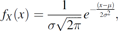
The histograms of the visual sensor in Fig. 6a and b show Gaussian-like distributions with bi-modality and unimodality in string and tree topologies. In general, it is reasonable to assume that an internet traffic follows the Exponential PDF for the transmission delay. However, our measurement does not follow the assumption. This is because the obtained histogram is not for a set of one packet delay but for the delay of one image file. For example, 20 KBytes image files are delivered by 20 separate packets, each of which has 1000 Bytes size. Therefore, we can not say that the transmission delay of 20 KBytes image follows the Exponential PDF. To explain more clearly why we get the Gaussian-like PDF, let us consider a statistic example where we pick up 20 samples from a population having an arbitrary PDF. Then, the sum of 20 samples becomes a random variable, and the random variable approximately follows Gaussian distribution according to the Central Limit Theorem (CLT) [14]. Similar to this example, we can say that the transmission delay of 20 KBytes image file is a random variable summing transmission delays of 20 separate packets, and the random variable follows a Gaussian PDF according to the CLT. Even if the distribution with bimodality is not the actual Gaussian PDF, we approximate the distribution as Gaussian in the SEA, which might give an estimation error in the SEA calculation.

Let X be the random variable for $x_{i}^{v 1}$ and $x_{i}^{v 2}$ . Then, X has PDF f_X(x) as follows.

f_{X} (x) = \frac{1}{σ \sqrt{2 π}} e^{- \frac{(x - μ)}{2 σ^{2}}},

(2)

where μ is the expected value and σG is the standard deviation.

For the acoustic sensor, the histogram is close to Gamma PDF with appropriate shape (k) and scale (θ) parameters. Let us define Y as the random variable for y_j. Then, Y has following PDF:

f_{Y} (y) = y^{k - 1} \frac{c^{y / θ}}{θ^{k} Γ (k)}, y > 0,

(3)

where k > 0, θ > 0. Note the Exponential PDF can be formulated from Gamma PDF with k = 1, θ =1/λ, where λ is a rate of the Exponential distribution. In order to simplify the random number generation for y_j in the SEA, we use Exponential PDF instead of Gamma PDF. The Exponential assumption is reasonable when an internet traffic generally follows the Exponential PDF. In the validation section, this simplification is proven to be reasonable. Finally, we can determine the PDF for Y as:

f_{Y} (y) = {\begin{cases} λ e^{- λ y}, y \geq 0, \\ 0, y < 0. \end{cases}

(4)

3.2. Formulation of the SEA

Based on the previous PDF approximation, we explain the details of the SEA in this section. SEA is composed of four modes, Right (R), Left (L), Both (B), and Unreachable (U) and two states, success (s) and fail (f). Each mode except U mode has two states.

When a server receives the multi-modal sensor data, it has to determine whether it uses the data and calculates the object coordinates. This procedure and determination criteria are illustrated in Section 2.4. Please remember that the visual compensation process is success when the capturing times of two visual sensors are later than the sampling time of the acoustic sensor and the next sampling time of the acoustic sensor is later than the feedback from the server as illustrated in Fig. 3a.

When we observe the traffic patterns appearing in the tracking system, we find out that there exist various patterns since the acoustic and visual sensors independently create the data, and the sensor traffic has different characteristics, i.e., the acoustic sensor uses UDP and visual sensors use TCP, the data sizes are different, and the transmission delay of each data is different. Even if the traffic behaviors are changed in times, we quantify the success case by defining three modes and two states according to the situations taking place in the tracking system as follows.

(1)
The capturing times of two visual sensors are later than the sampling point of the acoustic sensor. This case is defined by R mode like t₁ - t₇ interval in Fig. 5. In this case, the server can calculate the object coordinates and sends the feedback data to the acoustic sensor. If the feedback data reaches the acoustic sensor on time, then the acoustic sensor adjusts its PF parameters according to the feedback data, and this case is defined by s state. However, it could happen that the feedback arrives at the acoustic sensor after the next acoustic sampling has been sent to the server. This situation can occur due to a congested condition of a tracking network. This case is defined by f state. When the system is in s state, the SCR value increases by one.
(2)
The capturing times of the two visual sensors are earlier than the sampling point of the acoustic sensor. This case is defined by L mode like t₇−t₁₁ interval in Fig. 5. In this case, the server can NOT calculate the object coordinates. Instead, the server has to wait for the next frame arrivals from the visual sensors. If the next visual frames arrive before the next acoustic sensor data, the server uses the next visual frames to calculate the object coordinates and send the feedback containing the calculated coordinates to the acoustic sensor. Afterwards, the determination of s or f state is the same as (1).
(3)
The capturing time of one visual sensor is earlier than the sampling point of the acoustic sensor but the capturing time of another visual sensor is later than the sampling point of the acoustic sensor. This case is defined by B mode like t₁₁−t₁₅ interval in Fig. 5. In this mode, the frame of one visual sensor can be used in the localization algorithm but the other one should not be used. Like (2), a server can wait for the next frame arrivals from visual sensors for coordinate calculation; however, this mode gives confusion to the mode determination in the next round if the Δt_s value is short. Therefore, in the SEA algorithm, we assume the B mode always goes to the f state. Even if this seems to be a strong assumption, it is feasible to the SCR calculation of the SEA since the SEA has a memory-less property that can be illustrated as follows.

To determine whether any mode goes to s state, in other words, the SCR value increases by one, the SEA generates the random values from the pre-determined PDFs. In the next-round operation, the SEA does not use the previous random values, but newly generates the random values and uses them to determine the mode and state. This is the different point of the SEA algorithm from the real situations in which the next mode and state determination depend on the current behavior of the tracking system. This memory-less property is included in Algorithm 1.
(4)
When we observe the traffic patterns in the tracking system, we find out a special case that the transition from a mode to the other rarely happens. For example, the s state in R mode between t₁ and t₇ in Fig. 5 rarely yields R or B mode due to the traffic characteristics of the tracking network. We define this case as an unreachable mode, in short, U mode, and the SEA algorithm does not include the U mode case for SCR counting which makes the algorithm clear and simple. Please note that the above cases are the overall description for the mode and state determination. The sophisticated procedures that reflect the real situations are formulated by the transition rules of the SEA in Fig. 7 and the pseudo code of the SEA in Algorithm 1.

Figure 7.
Transition rules of the SEA.

In Fig. 7, each mode is represented by a colored rectangle, and the s and f states are indicated by the circle inside of the rectangle. For example, R_s and R_f stand for s and f states in R mode. In the figure, the solid arrow lines indicate possible mode-state transitions, and the dashed arrow lines stand for U mode. The transitions are allowed only from state-to-mode, and there are no mode-to-mode, state-to-state, and mode-to-state transitions since any state is following a mode as explained in (1), (2), and (3) in the beginning of this section.

The transition of the SEA is performed based on Δt_s, and random values for transmission delay, which are generated from the Gaussian and Exponential PDFs of random variables X and Y, X can take four different values: $x_{i}^{l}, x_{i}^{s}, x_{i + 1}^{l}$ , and $x_{i + 1}^{s}$ The subscript i and i + 1 imitate the current and next image frame captured by a visual sensor in a real situation. Whenever two visual sensors send the captured image frames, the transmission delays of the images depend on a current network condition. According to the size of the delay, we assign the superscripts l and s. For example, if the transmission delay of visual sensor 1 is larger than that of visual sensor 2 for i_th image, that is, $x_{i}^{v 1} > x_{i}^{v 2}$ , we determine l and s as follows:
$x_{i}^{l} \leftarrow x_{i}^{v 1}, x_{i}^{s} \leftarrow x_{i}^{v 2} .$
(5)

The SEA utilizes the next image frame, i.e., (i + 1)_th image, and the size of the delay is set by following the decision of the i_th image. For example, in case of Eq. (5) we have:
$x_{i + 1}^{l} \leftarrow x_{i + 1}^{v 1}, x_{i + 1}^{s} \leftarrow x_{i + 1}^{v 2} .$
(6)

The prediction of the next frame is possible in the SEA due to the random generation from the PDFs.

Algorithm 1:
Pseudo code of the SEA

The random variable Y takes a value y_j. In the transition rules, we use α to indicate what percent of $x_{i}^{v 1}$ and $x_{i}^{v 2}$ is slanted toward the right-hand side from the sampling time of acoustic sensor that is represented by the red dashed line in Fig. 5. For example, at t₁₅, around 60% of $x_{5}^{v 1}$ is slanted to the right-hand side of the red line; but around 20% for $x_{5}^{v 2}$ . In this case, α ≈ 0.6 for $x_{5}^{v 1}$ and α ≈ 0.2 for $x_{5}^{v 2}$ . Since it is difficult to determine α for each situation, we fix it to a constant value when we validate the algorithm.

In the remainder of this section, we will explain the details of the SEA by comparing Fig. 5 with Fig. 7. Figure 5 starts from R mode since the capturing times of the two visual sensors are later than the sampling point of the acoustic sensor. In other words, $x_{i}^{v 1}$ and $x_{i}^{v 2}$ are right-hand side of the red dashed line at t₁. According to Eq. (5), we have:
$x_{1}^{l} \leftarrow x_{1}^{v 1}, x_{1}^{s} \leftarrow x_{1}^{v 2},$
(7)
where $x_{1}^{v 1} > x_{1}^{v 2},$ . Since y₁ occurs within Δt_s, we have a success, and current state becomes R_s. Here, we can define a transition rule: R_s takes place if and only if $x_{1}^{l} + y_{1} \leq Δ t_{s}$ and $x_{1}^{s} + y_{1} \leq Δ t_{s}$ , which subsequently results in L mode in the next Δt_s period.

In Fig. 5, we can understand why the transition from R_s to B or R mode is unreachable. In other words, for R_s to B transition, the sampling of z₂ has to take place between t₄ and t₅. However, this case does not take place since the current state is R_s, and the arrival point of y₁ should exist after t₅. Due to the same reason, R_s can not be reachable to R mode. Similar to this example, we can figure out why L_s is unreachable to R and B mode.

We are now in L mode, and $x_{2}^{v 1}$ and $x_{2}^{v 2}$ are now used to determine the next status. Here, we require the next transmission delays $x_{3}^{v 1}$ and $x_{3}^{v 2}$ to determine a transition. Note that we do not know the next delays in real situations. However, in the SEA, we can obtain the estimate values for the next delays by using the pre-determined Gaussian and Exponential PDFs under the assumption that we have known the PDF parameters: μ and σG of Gaussian PDF, and λ of Exponential PDF. We are now able to generate the next delays $x_{3}^{v 1}$ and $x_{3}^{v 2}$ from the PDFs, and determine the current state. If following rule is satisfied, current state becomes L_s.
$α x_{2}^{l} + x_{3}^{l} + y_{2} \leq Δ t_{s} Λ α x_{2}^{s} + x_{3}^{s} + y_{2} \leq Δ t_{s} .$
(8)

Otherwise, the current state becomes L_f. Here, we assume $x_{2}^{v 1} > x_{2}^{v 2}$ , and according to Eqs. (5) and (6), the superscript l and s have been determined as follows.
$\begin{aligned} x_{2}^{l} \leftarrow x_{2}^{v 1}, x_{2}^{s} \leftarrow x_{2}^{v 2} \\ x_{3}^{l} \leftarrow x_{3}^{v 1}, x_{3}^{s} \leftarrow x_{3}^{v 2} . \end{aligned}$
(9)

Unfortunately, the time period (t₇, t₁₁) does not satisfy Eq. (8). Therefore, L_f becomes the current state. Now, we have to decide the next mode. We realize (t₇, t₁₁) period is under the following condition which is the third or-combined transition rule in C_Lf3.
$\begin{aligned} (α x_{2}^{l} < Δ t_{s} Λ α x_{2}^{s} < Δ t_{s}) Λ \\ (α x_{2}^{l} < x_{3}^{l} \leq Δ t_{s}) Λ \\ (α x_{2}^{l} + x_{3}^{l} + y_{2} > Δ t_{s}) Λ \\ (α x_{2}^{s} + x_{3}^{s} < Δ t_{s}) . \end{aligned}$
(10)

Equation (10) now results in B mode in the next Δt_s period. Once we enter the B mode, the next mode has f state as explained in the beginning of this section. For example, if we assume that $x_{4}^{l} + x_{4}^{v 1}$ and $x_{4}^{s} + x_{4}^{v 2}$ , the condition $α x_{2}^{s} + x_{3}^{s} \leq Δ t_{s}$ causes $x_{4}^{s}$ to start at the left-hand side from t₁₁ line. This leads to fail since it does not satisfy Condition 1.

Even though we illustrate the mode and state transition from one typical example, we believe the other transition rules in Fig. 7 cover almost all the transitions which appeared in the tracking system, which will be verified in Section 5.

Algorithm 1 describes the pseudo code of the SEA, which is derived based on the transition rules in Fig. 7. In the algorithm, we assume the population parameters for X and Y have already been known such that X has (μ_v1, σG_v1) and (μ_v2, σG_v2) for visual sensor 1 and 2, and Y has λ_y. Based on the parameters, we generate Gaussian random numbers from Eq. (2) and Exponential numbers based on Eq. (4). After we have five random numbers, we determine $x_{i}^{l}, x_{i}^{s}, x_{i + 1}^{l}, x_{i + 1}^{s}$ by comparing $x_{i}^{v 1}$ with $x_{i}^{v 2}$ . Then, modes and states are exchanged according to the transition rules.

In summary, the basic idea of the SEA is that we can estimate the tracking accuracy of the multi-modal tracking system if we can define the transmission delay of multi-modal sensors and the time point when the visual compensation process becomes a success. We obtain the PDFs from the transmission delay of the multi-modal sensors and derive the transition rules, by which we can decide whether visual sensors successfully assist the tracking error of an acoustic sensor. This procedure gives the other scientist the insight how to derive a numerical formula that helps to measure the tracking accuracy of their system to be installed.
4. Statistical Estimation and Adaptation Algorithm (SEA²)

In this section, we propose a Statistical Estimation and Adaptation Algorithm (SEA²) to answer the system maintenance problem mentioned in Section 2.7. If we are given a target SCR (t_scr) that represents a level of tracking accuracy, the objective of this algorithm is to achieve the t_scr in a realtime manner. SEA² uses the SEA to get the initial acoustic sampling interval. Therefore, we need to predict the population parameters of the PDFs to start the algorithm.

Figure 8 shows the procedural illustration of the SEA² that is composed of two Phases. The prediction of population parameters is done in Phase 1, and the automatic adaptation of acoustic sampling interval is performed in Phase 2.

Figure 8.

Procedural illustration of the SEA².

The SEA² is performed between acoustic sensors and a router based on two message types: PT_TSRQ and PT_TSRP. When we remind the tracking system configuration, the acoustic sensors and a router have n-to-1 mapping, where one router needs to control n acoustic sensors to adjust the acoustic sampling interval. In Phase 1, the router sends PT_TSRQ every Δt_a interval to synchronize the arrival of response message PT_TSRP from n acoustic sensors. Generally, we set up Δt_a to a larger value than the acoustic sampling interval, so that a number of compensation processes are performed within Δt_a. As soon as acoustic sensors receive the request packet, they set the sampling interval to $\frac{Δ t_{s}^{c}}{2^{i}} (i = 0, 1, 2, \dots)$ which means an exponential decrease of a constant sampling interval $Δ t_{s}^{c}$ . The exponential factor i increases by 1 from 0 whenever acoustic sensors receive PT_TSRQ, and $Δ t_{s}^{c}$ is set to a reasonably large value. The main reason we use the exponential decrease is to fast advance to Phase 2, which is beneficial for finding the acoustic sampling interval to achieve t_scr. Actually, SEA is more sensitive not to the size of the population parameters but to the acoustic sampling interval, so that we do not have to consume much time to obtain accurate population parameters in Phase 1. Note that we achieve 100% SCR when the acoustic sampling interval is sufficiently large. Therefore, as we exponentially reduce the sampling interval, the SCR also decreases in proportion to the interval. Since acoustic sensors have different sizes of sampling interval within Δt_a, they perform n_i number of sampling, which is denoted by $n_{i} \frac{Δ t_{s}^{c}}{2^{i}}$ . In Phase 1, acoustic sensors measure the SCR value within $n_{i} \frac{Δ t_{s}^{c}}{2^{i}}$ , and send the information to the router.

Let us define the estimated means and standard deviations of X in Phase 1 as ( $({\hat{μ}}_{v 1}, {\hat{σ}}_{v 1})$ ) and ( $({\hat{μ}}_{v 2}, {\hat{σ}}_{v 2})$ ), and the estimated mean of Y as ${\hat{λ}}_{y}$ . To obtain $({\hat{μ}}_{v 1}, {\hat{σ}}_{v 1})$ and $({\hat{μ}}_{v 2}, {\hat{σ}}_{v 2})$ , the server piggybacks the transmission delays of visual images in the feedback packet. When a router is relaying the feedback to acoustic sensors, it can obtain the transmission delay, and subsequently ( $({\hat{μ}}_{v 1}, {\hat{σ}}_{v 1})$ ) and ( $({\hat{μ}}_{v 2}, {\hat{σ}}_{v 2})$ ). The acoustic sensors measure the SCR and transmission delay from the server to itself, and send them to the router by using PT_TSRP. Then, the router uses the received delay to obtain the ${\hat{λ}}_{y}$ . This procedure continues until we have SCR < γ, where γ is a confidence level and set by a constant value. The estimated parameters for X and Y are obtained from averaging the measured delays so far. Now, we can run the SEA to obtain an initial acoustic sampling interval $Δ t_{s}^{0}$ . For the input parameters of the SEA, we use the estimated population parameters as follows.

\begin{aligned} μ_{v 1} \leftarrow {\hat{μ}}_{v 1}, σ_{v 1} \leftarrow {\hat{σ}}_{v 1}, \\ μ_{v 2} \leftarrow {\hat{μ}}_{v 2}, σ_{v 2} \leftarrow {\hat{σ}}_{v 2}, \\ λ \leftarrow {\hat{λ}}_{y} . \end{aligned}

(11)

Algorithm 2:

Adjustment algorithm of the acoustic sampling interval $Δ t_{s}^{i}$

Phase 2 starts with sending $Δ t_{s}^{0}$ from a router to acoustic sensors. Different from Phase 1, the router receives the SCR from the acoustic sensors for κΔt_a and controls the sensors to adapt the sampling interval $Δ t_{s}^{i} (i = 1, 2, \dots)$ based on Algorithm 2, where κ is a constant positive integer. We maintain $Δ t_{s}^{i}$ for a longer period κΔt_a since the tracking network fluctuates in times and it is not sufficient to determine the object sampling interval only by observing one Δt_a period. In Algorithm 2, in order to do a fast adjustment of the sampling interval from the continuous miss from t_scr, we use exponential increase and decrease of the acoustic sampling interval by δ2^e1 or δ2^e2, where e₁ and e₂ alternately increase according to their conditions, and δ should be set to a proper value. If δ is too small, we do not get the advantage of fast increase and decrease; otherwise, the measured SCR keeps deviated from the t_scr. If the SCR measured for κΔt_a is less than t_scr − ∊, we perform increment; otherwise, decrement is done. The ∊ is a statistical tolerance error which reflects the fluctuation of tracking network traffic. We recommend 5% tolerance error to sufficiently include the network fluctuation.

5. Algorithm Validation and Discussion

In order to conduct the validation of the proposed algorithms, we use NS-2 simulator [9]. We configure string and tree-based tracking system as shown in Fig. 9 to validate the correctness of both algorithms. Even if the configuration is simple in terms of routers, the tracking complexity is affected by the number of acoustic sensors and tracking objects. Therefore, we believe it suffices to configure a line of routers for characterizing the tracking system and validating the algorithms. Each acoustic sensor is sampling 5 objects. 20 Kbytes or 40 KBytes visual image is generated by visual sensors and delivered by 1000 Bytes TCP packets. We install a multiple channel for router-router communication, and a single channel for acoustic sensor-router communication. In the figure, different colors represents different channels. For wireless links, we use 54Mb/s 802.11a with 0.0005 of uniformly distributed Bit Error Rate (BER). In the string scenario, we set up 5 routers (R0 to R4) each of which has three acoustic sensors. The processing server is connected to the last mile router R4, and two visual sensors are attached onto R1 and R3. For the tree scenario, we use 8 routers (R0 to R7) among which only R0 to R5 have two acoustic sensors, and R6 and R7 only relay sensor traffic. We assume two branches of the tree do not guarantee the line-of-sight characteristics of visual sensors, so that we install two visual sensors for each branch.

Figure 9.

Simulation scenarios for the object tracking system. Acoustic sensor, visual sensor, and router are denoted by A_i, V_i, and R_i, respectively. Due to a line-of-sight characteristics of visual sensors, we install 4 visual sensors in the tree topology.

5.1. Validation of the SEA

We verify that the SEA accurately estimates the SCR by comparing simulation results with mathematical calculation of the SEA. To do this work, we obtain SCR results (%) for five different acoustic sampling intervals (Δt_s): 0.1, 0.15, 0.2, 0.3, 0.4. In order to observe precise variation in short Δt_s cases, we include the result of Δt_s = 0.15. It is possible to track high speed objects and obtain more accurate tracking information on the same objects if Δt_s gets shorter. As the visual image size increases, we also get more information from the image, so that we can increase the accuracy of visual localization algorithm at a server.

Figure 10 plots the SCR results from the simulation and numerical calculation. We first observe the SCR from simulations drawn by solid lines with black points. The plots indicate that small SCRs are achieved in acoustic sensors far from the server, short Δt_s, and small visual image size. These results are obvious since the Condition 1 to Condition 3 in Section 2.4 and Section 3 are well satisfied under the above tracking system environment. Especially, Fig. 10d shows that all the SCRs are very small since the tree scenario and larger image size cause non-synchronization between multi-modal sensors. The SCR estimates from the SEA are drawn by dotted lines with white points in the figure. For the input population parameters (μ_v1, σG_v1), (μ_v2, σG_v2), and λ_y for the SEA, we use the measured values from simulations. We can observe that almost all SEA calculation results are close to the simulation results except for some cases like Δt_s = 0.15 in Fig. 10a, and Δt_s = 0.3 in Fig. 10b and c, which have around 20% deviation from the simulation results.

Figure 10.

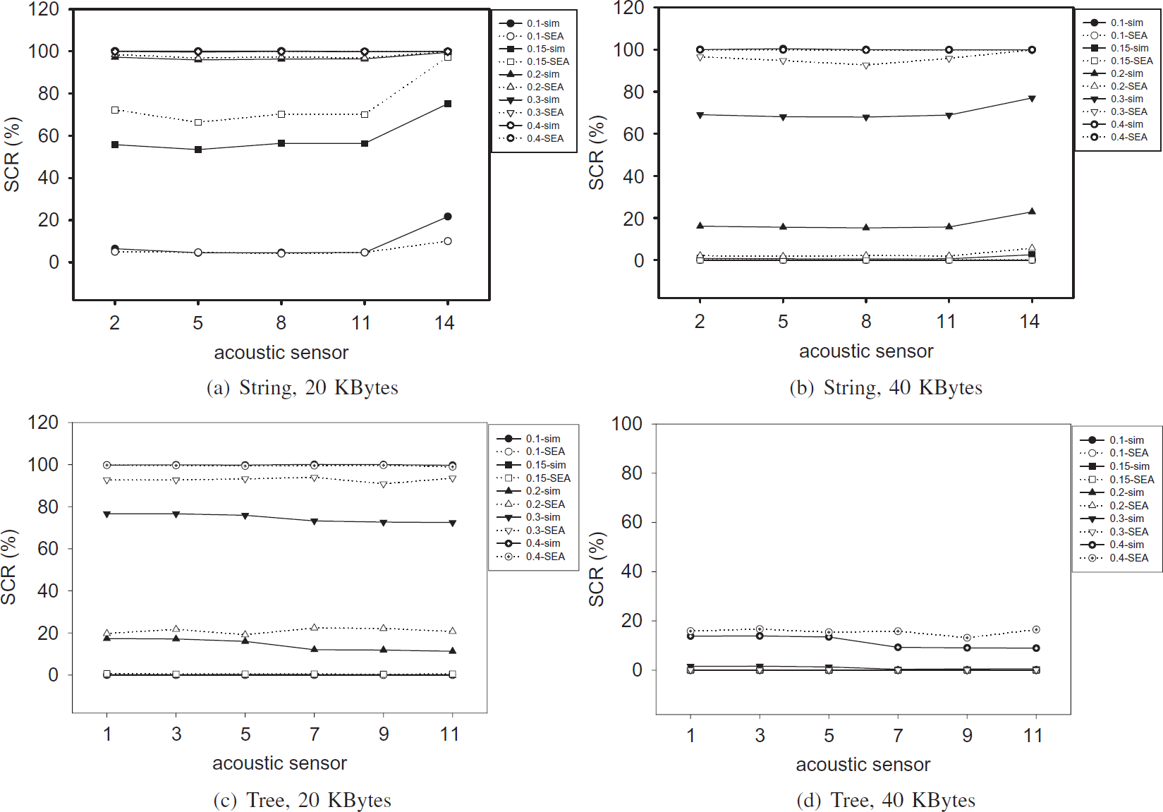
SCR values achieved by simulations and mathematical calculation of the SEA.

5.2. Validation of the SEA²

For the validation of SEA², we observe how the SEA² automatically adapts the acoustic sampling interval to accomplish a given t_scr. To do this work, we run NS-2 simulations for 2400 s, and measure the sampling interval variations every 10 s interval. In Phase 1, the confidence level γ is set to 90%, and SEA² starts its running by setting the initial sampling interval $Δ t_{s}^{c}$ as 1.2 second. In Phase 2, the statistical tolerance error ∊ is set to 5%, and δ for controlling the exponential increase and decrease level is set to 0.01. We fix κ = 4 for SCR observation interval.

Figure 11 shows the automatic adjustment of the acoustic sampling interval to achieve t_scr = 90%. To obtain the plots, we run simulations ten times and take average values. The results are observed at each router to prevent the plotting of all the acoustic sensors' sampling intervals, which is reasonable since the router controls the acoustic sensor behaviors within its communication range. In Fig. 11 a, we understand R0 to R3 achieve 90% SCR at around Δt_s = 0.19. However, R4 accomplishes it at shorter value, Δt_s = 0.16 since R4 directly connects to the server and fast exchanges sensor data with the server. Note we achieve 60% SCR at Δt_s = 0.15 and around 100% SCR at Δt_s = 0.2 in Fig. 10a. This indicates that SEA² correctly adapts the acoustic sampling interval to achieve 90% target SCR. When the visual image size increases to 40 Kbytes in string topology as shown in Fig. 11b, Δt_s saturates to between 0.30 and 0.35 after fluctuating for initial simulation time duration. The correctness of this adaptation is also verified in Fig. 10b. As a tracking scenario is complicated to the tree and the file size is large, the Δt_s shows a larger variations as shown in Fig. 11c and d. However, the adaptation to achieve 90% SCR is verified to be correct if we compare the results with Fig. 10c and d. In the worst scenario like tree and 40 Kbytes image size, 90% SCR is achieved when Δt_s > 0.65. From these results, we have knowledge that we should reduce the visual image size to increase the successful compensation rate in case we have to construct a complicated tracking environment.

Figure 11.

Acoustic sampling interval variation in the SEA², where t_scr = 90%.

In order to observe real-timing adaptation capability of the SEA², we change t_scr during simulations, and observe the acoustic sampling interval variations as shown in Fig. 12, where we include only 20 Bytes image cases for string and tree topologies. When simulations start, we fix t_scr to 30%. After simulation time reaches 800 seconds, we change the t_scr to 60%. Finally, t_scr = 90% when the time becomes 1600. In Fig. 12a, we observe SEA² is efficiently adaptive to the changes of t_scr. The Δt_s variations at 30% and 60% t_scr are around 0.02 in worst case, which is expected to be tolerable when we compare it with the exponential increase and decrease level (δ) which is set to 0.01. Figure 12b indicates SEA² provides confidential acoustic sampling interval adaptation mechanism even if the acoustic sampling interval variation in tree is larger than that of the string scenario.

Figure 12.

Acoustic sampling interval variation in the SEA². t_scr is changed to 30, 60, and 90% during the simulations.

6. Conclusion

This paper has proposed a Statistical SCR Estimation Algorithm (SEA) to estimate the number of success of visual compensation anticipated in a multi-modal tracking system. The SEA takes the acoustic sampling interval and transmission delays of multi-modal sensor data as the algorithm ic parameters. To formulate the algorithm, we investigate the transmission delays between the multi-modal sensors and the server. From the observation, the delays are modeled by Gaussian and Exponential Probability Density Function (PDF). From the PDF, the SEA generates random values to mimic the delays in real environment, and based on the results, it changes its status according to the transition rules. There are R, L, B, and U modes and s and f states in the transition. We have shown that the SEA can properly approximate the number of success in the visual compensation by hand calculation.

Another proposed algorithm, the Statistical and Estimation and Adaptation Algorithm (SEA²), is suitable for answering how to maintain the tracking system at a certain level of tracking accuracy. The SEA² maintains the tracking accuracy by automatically adapting acoustic sampling interval since the accurate tracking depends on the success in the visual compensation. The algorithm is composed of Phase 1 and Phase 2. In the first Phase, it runs the SEA to obtain an initial sampling interval. Then, exponential increase and decrease of the obtained interval are performed to fast adapt the acoustic sampling interval to accomplish the target tracking accuracy level. From the simulations, we have shown that the SEA² well adapts the sampling interval of acoustic sensors.

References

Lee

Hong

Cho

W.D.

, “Acoustic Sensor Based Multiple Objects Tracking with Visual Information Association,” Technical Report-MSDL-SUNYSB, http://msdl.ee.sunysb.edu/~skjung/papers/AcousticSensor.pdf.

Zotkin

D. N.

Duraiswami

Davis

L. S.

, “Joint Audio-Visual Tracking Using Particle Filters,” EURASIP Journal on Applied Signal Processing, p. 549–552, 2003.

Vermaak

Blake

, “Nonlinear filtering for speaker tracking in noisy and reverberant environments,” IEEE Int. Conf. Acoust., Speech, Signal Processing (ICASSP-01), Salt Lake City, UT, May 2001.

Ward

D. B.

Williamson

R. C.

, “Particle filter beamforming for acoustic source localization i a reverberant environment,” Proc. IEEE Int. Conf. Acoust., Speech, Signal Processing (ICASSP-02), Orlando, FL, May 2002.

Jue

Le Cadre

J. P.

Perez

, “Sequential monte carlo methods for multiple target tracking and data fusion,” IEEE Trans. Signal Processing, vol. 50, pp. 309–325, Feb. 2002.

Arulampalam

Maskell

Gordon

Clapp

, “A Tutorial on Particle Filters for Online Non-linear/Non-gaussian Bayesian Tracking,” IEEE Transactions on Signal Processing, 50(2): 174–188, Feb. 2002.

Jung

Lee

Hong

, “On Addressing Network Synchronization in Object Tracking with Multiple Sensors,” KSII Transactions on Internet and Information Systems, vol. 3, no. 4, pp. 344–365, August 2009.

Hong

Lee

Athalye

Djuric

P. M.

, “Design Methodology for Domain-Specific Parameterizable Particle Filter Realizations.” IEEE Transactions on Circuits and Systems-1, 2007.

Network Simulator-2, http://www.isi.edu/nsnam/ns.

10.

Stanacevic

Cauwenberghs

, “Micropower Gradient Flow acoustic Localizer,” Proc. of Solid-State Circuits Conf. (ESSCIRC03), pp. 69–72. 2003.

11.

Lee

Hong

Park

Cho

W. D.

, “Object Tracking Based on RFID Coverage and Visual Compensation in Wireless Sensor Network,” Proc. of the IEEE International Symposium on Circuits and System, 2007.

12.

Lee

Jung

Kyong

Deng

Hong

Cho

W.D.

, “Data Traffic Analysis in Wireless Fusion Network with Multiple Sensors.” Proc. of IEEE International Midwest Symposium on Circuits and Systems (MWSCAS), Montreal, Canada, August 5–8, 2007.

13.

4XEM PTZ Pan/Tilt/Zoom IP Network Camera. http://www.4xem.com/products/wired/IPCAMWPTZ/index.html.

14.

Leon-Garcia

, “Probability and Random Processes for Electrical Engineering,” Addision Wesley.

Statistical Estimation and Adaptation for Visual Compensation in Object Tracking

Abstract

Keywords

1. Introduction

2. Background and Motivation

2.1. Tracking by Multi-modal Sensors

2.2. Target Application Model

3. Statistical SCR Estimation Algorithm (SEA)

References