Sage Journals: Discover world-class research

Abstract

This paper deals with the issue of non-model-based position regulation for the dynamic compensation robotic system (DCRS), which has been proposed for cooperating with the existing main robotic systems, such as the common serial robotic arms, to accomplish high-speed and accurate manipulations. The dynamic compensation concept is realized by fusing a high-speed & light-weight compensation actuator as well as endpoint closed loop (ECL) configured high-speed cameras. Within the context of the DCRS, the coarse motion, which is realized by the main robotic system, usually gives rise to negative dynamic impact on the compensation actuator that is configured to accomplish the fine motion. Through the analysis of a simplified model for the coupled two-plant system, relative velocity information between the two plants is found to play a role in the first order derivative of the displacement error. With the use of the relative position information from high-speed visual feedback, this paper proposes a new pre-compensation fuzzy logic control (PFLC) approach for control of the compensation actuator. The PFLC method is model-independent and is realized with a cascade fuzzy inference structure that conveniently integrates the relative velocity term between the two plants into the error regulation, and therefore realizes the partial counteraction of the disturbance from the main robot easily without knowing the explicit mathematical models of the system. Comparison works between the proposed PFLC and approaches that take no consideration of the relative velocity information, such as proportional-derivative (PD) control and conventional fuzzy logic control, are conducted. Simulations and experiments show the consistent effectiveness of the proposed approach.

Keywords

Dynamic Compensation High-speed Visual Feedback Model-independent Control Pre-compensation Fuzzy Logic Control

1. Introduction

High-speed and accurate position regulation for the traditional robotic system is a challenging issue in the robotic control theme. This is because not only does the mechanism have some defects, such as backlash, but also the existing control methods cannot easily accommodate the dynamics issue for unknown working conditions, especially under high-speed manipulations.

Most commercially available industrial robots are equipped with the so-called non-model-based controllers, as their control systems are treated as decoupled systems and dynamics are neglected [1]. Such approximation is acceptable for low-speed motion since Coriolis and centripetal forces are limited due to powerful motors and high gear reductions [1, 2]. However, this approach cannot be applied to high-speed motions [3]. On the other hand, model-based approach has been frequently studied to realize dynamic compensation by identifying the parameters of the dynamic model [1, 4]. For the model-based approach, usually computation is too complex to realize high-speed compensation. Besides, physical values of the dynamic model are difficult to estimate and often not accurately known. Moreover, these parameter values may change with the robot's service time or robot configurations.

In another approach, a small robot mounting on the robotic arm, known as the macro-micro architecture [5, 6], is employed. The macro-micro approach has been proposed to apply to rigid manipulators for increasing system bandwidth, as well as to flexible manipulators for suppressing bending vibrations and improving dynamic tracking performance (e.g., [7, 8]). Since the micro-manipulator is mounted on the macro-manipulator, the system is dynamically coupled, especially for flexible manipulators [9, 10].

Usually, for a light-weight micro-manipulator, the coupling dynamical interaction to the macro part is negligible as the inertia of the macro part is much greater than that of the micro part [11, 12]. In [11], the dynamic effect of the macro part to the micro part is represented by a disturbance force, and by choosing a large proportional gain factor of the PD controller for the micro-manipulator, the disturbance force can be reduced and the system stability can be proved. It should be noted that this approach is model-independent and it represents a kind of method that doesn't need to model the system's dynamics. Although this approach is very simple and easy for implementation, it cannot be used as a general approach for high-speed positioning. In [13] and [14], the dynamic trajectory tracking problems have been studied, and the dynamics of the system are taken into account with a fine model including the macro-manipulator's deformation. In [13], a simple PD controller is assigned for the macro-manipulator, and a non-linear dynamic compensating control law is applied to the micro-manipulator. In [14], a different strategy is adopted by applying the PD control to the micro part, and adopting the nonlinear controller for the macro part to damp out vibrations. In both approaches, the trajectory planner is needed for the macro-manipulator. These approaches obtained good performance for dynamic compensation, yet the modelling for the system's dynamics is not easy. In [15, 16], a feedback controller based on the discrete-time-domain disturbance observer is established to compensate for external disturbance mainly from the coarse positioner. Basically, the disturbance observer is a high gain technique, and the unmodelled dynamics limit the allowable loop gain if robustness is to be retained. Correspondingly, the performance will be limited.

With the advantages of the high-speed visual feedback that provides the overall real-time information, a non-model-based dynamic compensation concept has been proposed by fusing a high-speed & light-weight compensation actuator and high-speed visual feedback in terms of relative position information between target and robot [17]. Under the proposed dynamic compensation concept, high-speed as well as accurate positioning towards a target is supposed to be accomplished without knowing much about the system's mathematical models. However, the problem that the compensation actuator for fine positioning is dynamically disturbed by the main robot's motion has not been tackled as yet. This paper proposes a pre-compensation fuzzy logic control method to address this issue. The reason for adopting the fuzzy logic approach in this paper is that a model-independent cascade fuzzy inference structure that integrates the relative velocity term (which is found to play a role in the first order derivative of the displacement error through later analysis of the system's overall behaviour) into the overall positioning regulation can be realized very conveniently to partially counteract the disturbance. ‘Pre-compensation’ lies in the methodology that the first layer of the fuzzy inference system realizes the combination of the velocity information of the two plants to compensate for the disturbance part within the displacement error, which has been brought by the main plant's motion.

It should be noted that since this paper focuses on the fundamental problem (counteraction of the nonlinear disturbance from the main robot) of the proposed dynamic compensation robotic system, we will only conduct the analysis as well as evaluation on 1-DOF DCRS – we think however that the result in this work is instructive in realizing a multi-DOF DCRS.

The rest of the paper is organized as follows. First, the concept of the dynamic compensation as well as the designed 1-DOF DCRS testbed is introduced in Section 2. Second, a simple cart model with the motion analysis, as well as the pre-compensation fuzzy logic control method and its implementation are described in Section 3. Third, in Section 4 and Section 5 a simulation study as well as experimental evaluations are conducted by comparing our method with two other model-independent methods that take no consideration of the relative velocity information including PD control and conventional fuzzy logic control. Finally, the conclusions of this work are given in Section 6.

2. Dynamic compensation robotic system

2.1 The dynamic compensation concept

For high-speed operations, defects such as vibration due to large inertia of the robotic system as well as mechanical backlash, would reduce the performance. As shown in Figure 1, the concept of dynamic compensation is to dynamically compensate for the robotic system's motion defects under high-speed visual feedback information through two aspects. Firstly, the high-speed compensation actuator with small inertia offers the necessary DOFs to compensate for the system's motion defects. The high-speed feature enables it to realize quick response during the system's dynamical converge, which is always realized in a very short period. Secondly, high-speed cameras are adopted to provide the relative position information between robot and target. As for the traditional robotic control, the local feedback information, such as the joint space feedback, is adopted for the global position regulation by applying the robotic system's kinematic and dynamic models, which actually act as the indirect approach. Here, in the proposed dynamic compensation concept, we directly adopt the global feedback information between the robot and the target by applying high-speed cameras that work at the frequency of 1000 Hz.

Figure 1.

The dynamic compensation concept, which includes two aspects: high-speed visual feedback in terms of the relative position between robot and target; a light-weight & high-speed compensation actuator (the main robot usually suffers from the dynamic defects such as vibrations under high-speed positioning)

It should be pointed out that although the dynamic compensation concept is somehow similar to the traditional macro-micro approach in related works [5 -10, 13], there are several different issues as follows:

High-speed visual feedback that offers the relative position information between robot and target is one important aspect of the proposed dynamic compensation concept, whereas the traditional macro-micro system itself does not involve a global high-speed visual feedback;

In order to realize high-speed and accurate regulation, rather than dealing with the complicated dynamic models of robot systems, we focus on developing model-independent control laws for easy implementation and for general applications in the proposed dynamic compensation concept.

2.2 1-DOF testbed

In order to study the basic motion control in the context of DCRS, we designed a 1-DOF DCRS testbed as shown in Figure 2. The testbed includes a main robot (linear motor actuator GLM1G-075 made by THK) that has a large work space and has been originally adopted for slow & accurate motion. The compensation actuator (QUICKSHAFT® linear DC-Servomotor LM1247–040-ll made by FAUHABER) is capable of high-speed motion with a small work range. Hereafter, we will refer to the main robot as the main plant, and the compensation actuator as the compensation plant. Specifications for the testbed are shown in Table 1. An eye-to-hand configured high-speed camera (Photron IDP-Express R2000) observes the motion patterns of the two plants at a frequency of 1000 Hz with the image size of 512×512. The regulation point is represented by a white LED light that is mounted on the compensation plant. The feature point for the main plant is represented by a blue LED light.

3. Pre-compensation fuzzy logic control (PFLC)

In order to illustrate the control issue, we firstly introduce a simplified model for the 1-DOF dynamic compensation robotic system.

Table 1.

System specification for the testbed

	Main plant Compensation plant
Max. vel. (m/s)	2.0	2.9
Max. acc. (m/s²)	3.0	148.5
Stroke (mm)	750	80

Figure 2.

The 1-DOF dynamic compensation testbed

3.1 A simple cart model

A simplified cart model consisting of the lower main plant and the upper compensation plant is shown in Figure 3. The system only conducts horizontal motion. Let us assume that the compensation plant could not move off from the main plant and the compensation plant's mass is m, which is far lighter than the main plant's mass M (m » M). The camera's focal length and scaling factor (pixel/meter) is f and α respectively, and the constant distance between the camera and robotic system is z (z >0). Hereafter, we will refer to the regulation point's position as x^c and the main plant's position as x_M^c in the fixed inertia frame Σ_c.x^M is the regulation point's position in the reference frame of Σ _M , which is attached to the main plant. Let F_M, F_m represent applied force on the main plant and compensation plant respectively.

In order to address the control issue, we make several assumptions about the system as follows: (1)

The applied force on the compensation plant F_m is calculated with respect to the frame Σ_M. Since the regulation point is set on the compensation plant, it will follow the combined motion of the main plant and the compensation plant.

(2)

The static friction force F_s between the main plant and the compensation plant is sufficiently large and there will be no relative motion between the two plants if the compensation plant is not activated by F_m.

(3)

The interaction force from the compensation plant to the main plant is sufficiently small and is negligible.

In order to comply with the second assumption, a suitable static friction force can be obtained between the main plant and the compensation plant by assembling these two appropriately. By adding some extra weight on the main plant to increase the inertia, the interaction force from the compensation plant can be negligible to come to the third assumption.

Figure 3.

A simplified cart model for the 1-DOF DCRS

The regulation point is initialized at x_s^c, and the target position is at x_d^c. Let us assume that during the whole motion range, the regulation point, the target point as well as the feature point for the main plant are all visible to the high-speed camera. Since the system only conducts horizontal motion, we can then make the projection from world position x^c to the image position ζ, by

ξ = \frac{f α}{z} \cdot x^{c} ​ = ​ ​ ​ λ \cdot x^{c}

(1)

We divide the regulation of x^c from x_s^c to x_d^c into two phases, firstly to regulate the system to move as a whole from x_s^c to x_p^c; secondly to regulate the compensation plant from x_p^c to x_d^c. x_p^c is the separation position for dividing these two phases. Let the constant distance from x_p^c to x_d^c be δx^c (δx^c ≥ 0), which is smaller than the stroke of the compensation plant. Let e_c = ξ _c – ξ _d be the image error between the regulation point and the target, and e_p = ξ _c -ξ _p be the image error between the regulation point and the separation position.

For the general case, suppose the control law for the first phase is the simple proportional-derivative (PD) control as

F^{'} = - K_{v} \cdot {\dot{e}}_{p} - K_{p} \cdot e_{p}

(2)

where K_v K_p are the positive gain factors, and F′ is the force applied on the main plant to drive the whole system. Once the image error e_p reaches zero, the regulation moves into the second phase. As for the dynamics of the system, we have:

\begin{array}{l} m \cdot {\ddot{x}}^{M} = F_{m} - F_{r} \\ ​ \\ (m + M) \cdot {\ddot{x}}_{M}^{c} = F_{M} + F_{r} \end{array}

(3)

where F_r represents the kinetic friction force between the two plants.

For the main plant that is supposed to stop around ξ _p , in order to keep the flexibility of the proposed approach, we keep the PD control law for the main plant as

F_{M} = - K_{v} \cdot {\dot{e}}_{M} - K_{p} \cdot e_{M}

(4)

where e_M = ξ _M – ξ _p with ξ _M representing the image position of the main plant's feature point.

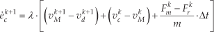
Note that during the second phase, e_c is the projection of combinational motions, including the main plant's motion, the relative motion between two plants, and the target's motion if we consider the general case. The derivative of e_c (ė_c) at a particular time, for instance at the time of k + 1, is

{\dot{e}}_{c}^{k + 1} = λ \cdot (v_{c}^{k + 1} - v_{d}^{k + 1})

(5)

where v_c^k+1,v_d^k+1 refers to the velocity of the regulation point and the target point at time k + 1 respectively. Suppose at time k, the applied force on the compensation plant and main plant to be F_m^k, F_M^k respectively; for the velocity of the regulation point, we have

v_{c}^{k + 1} = v_{c}^{k} + (\frac{F_{m}^{k} - F_{r}^{k}}{m} + \frac{F_{M}^{k} + F_{r}^{k}}{m + M}) \cdot Δ t

(6)

where, Δt is the control cycle time. Similarly, we have the velocity of the main plant at time k + 1 as

v_{M}^{k + 1} = v_{M}^{k} + \frac{F_{M}^{k} + F_{r}^{k}}{m + M} \cdot Δ t

(7)

Combining Equations (5), (6) and (7), we have

{\dot{e}}_{c}^{k + 1} = λ \cdot [(v_{M}^{k + 1} - v_{d}^{k + 1}) + (v_{c}^{k} - v_{M}^{k}) + \frac{F_{m}^{k} - F_{r}^{k}}{m} \cdot Δ t]

(8)

Since we have v_p = v_d, Equation (8) can be rewritten as

{\dot{e}}_{c}^{k + 1} = {\dot{e}}_{M}^{k + 1} + ({\dot{e}}_{c}^{k} - {\dot{e}}_{M}^{k}) + λ \cdot \frac{F_{m}^{k} - F_{r}^{k}}{m} \cdot Δ t

(9)

Equation (9) shows that at the time of k +1, the derivative of the displacement error e_c has relations to three parts, namely the derivative of the error e_M at time k + 1, the difference between ė_c and ė_M at time k, as well as the applied force on the compensation plant at time k.

Considering the case that the simple PD control is applied to the compensation plant as

F_{m} = - C_{v} \cdot {\dot{e}}_{c} - C_{p} \cdot e_{c}

(10)

where C_v, C_p are positive gain factors. Note that for the PD approach, the applied force F_m at time k is a function of ${\dot{e}}_{c}^{k}$ and e_c^k. More specifically, regarding Equation (9), the PD approach only makes use of the third term to realize the regulation of the displacement error. Therefore, under PD control, regulation of the compensation plant would be greatly affected by the nonlinear dynamics of the main plant, as revealed by the second term $ė_{c}^{k} - ė_{M}^{k}$ of Equation (9) while performing high-speed motions.

In the next part, based on the scope of developing model-independent control laws for dynamic compensation robotic system in this study, we shall take the advantage of the fuzzy logic method to realize a sophisticated control approach for the compensation actuator. The motivation for adopting the fuzzy logic method is that when compared with the classical model-based approach, it needs no intricate mathematical models, but only a practical understanding of the overall system behaviour (obviously, the system behaviour here has been analysed and is shown by Equation (9)).

3.2 The concept of PFLC

The fuzzy logic method is able to simultaneously handle numerical data and linguistic knowledge. It differs from classical logic in that statements are no longer black or white, true or false, on or off. In traditional logic, an object takes on a value of either zero or one. In fuzzy logic, a statement can assume any real value between 0 and 1, representing the degree to which an element belongs to a given set. The fuzzy logic control method has been successfully applied in fields such as automatic control, data classification, decision analysis, expert systems, and computer vision [18, 19].

As for the concrete task of regulating the compensation plant under high-speed visual feedback in this paper, a conventional fuzzy logic control system that takes ė_c^k and e_c^k as the input and F_m^k as the output at the time of k can be developed. Compared with the simple PD control illustrated above that basically fits for linear systems, the conventional fuzzy logic approach may be a suitable approach to handle the nonlinear behaviour of high-speed motion compensation system. But the same problem as has been illustrated for the PD method also exists for the conventional fuzzy logic approach since it does not consider the nonlinear disturbance from the main plant.

If we go back to Equation (9), we can see that at the time of k, the second term ${\dot{e}}_{c}^{k} - {\dot{e}}_{M}^{k}$ , as a matter of fact, can be evaluated from the high-speed visual feedback information. In order to have a better control of ė_c at the coming time k + 1, we can actually take the factor ${\dot{e}}_{c}^{k} - {\dot{e}}_{M}^{k}$ into consideration for generating the output force F_m at the time of k rather than only considering ${\dot{e}}_{c}^{k}$ and e_c^k. In other words, we can realize pre-compensation for the compensation plant by using ${\dot{e}}_{c}^{k} - {\dot{e}}_{M}^{k}$ to partially counteract the dynamic impact from the main plant, although the first term of Equation (9) (which is related to a feedforward control) will not be taken into consideration in this study. On basis of the conventional fuzzy logic method, the pre-compensation fuzzy logic control (PFLC) approach is proposed. The block diagram of the proposed PFLC is shown in Figure 4. Compared with conventional fuzzy logic control, the innovation point of the proposed method is that it also takes into consideration of the main plant's motion with a cascade fuzzy logic model. Through the feedback information of the main plant's motion, the nonlinear dynamic effect on the compensation plant can be partially compensated simultaneously while the compensation plant is regulated to the target position. The proposed PFLC method is a direct regulator to the plant rather than a gain tuner that has to be combined with some other control laws as in [20, 21], thus it is much easier to implement.

The PFLC includes two cascade fuzzy inference systems (FIS), one is for pre-compensation (referred to as FIS_1 hereafter) and the other is for error regulation (referred to as FIS_2). FIS_1 is actually combining the velocity information of the main plant and the compensation plant through high-speed visual feedback. The output of FIS_1 can then be taken as one input to the FIS_2 to generate the output force for driving.

3.3 Implementation of PFLC

The implementation of a fuzzy logic control system basically includes the steps of fuzzification, rule evaluation and defuzzification. For both FIS_1 and FIS_2, the universe of discourse for each input is partitioned into seven fuzzy sets: NL (‘negative large’), NM (‘negative medium’), NS (‘negative small’), ZE (‘zero’), PS (‘positive small’), PM (‘positive medium’) and PL (‘positive large’). Both FIS_1 and FIS_2 have two input variables and one output variable. For FIS_1, the two input variables are ė_M and ė_c representing the image error's velocity information relating to the main plant and the compensation plant respectively, the output is referred to as ė_com. For FIS_2, the input variables are the image error e_c and the output of FIS_1. The fuzzification is to map each crisp input over all the qualifying membership functions required by the fuzzy rules. For easy implementation, the simplest triangular membership function is adopted for the input ė_M, ė_c and e_c as shown in Figure 5. The universe of discourse for each input variable has been roughly calibrated.

After the step of fuzzification, the fuzzy rules are designed for FIS_1 and FIS_2. Under the ‘zedeh AND’ fuzzy combination operator, the designed fuzzy associate memory matrices (FAMM) for FIS_1 and FIS_2 are shown in Table 2 and Table 3 respectively. Each element of the FAMM refers to one If-Then rule statement. For instance, for the element FAMM-1 (1,1) : NL, means:

‘If ė_M is NL AND ė_c is NL Then output is NL’

As for the output variables in FIS_1 and FIS_2, the universe of discourse is partitioned into seven fuzzy sets with each attribute being described by the singleton membership functions as shown in Figure 6. The seven fuzzy sets are the same as the input fuzzy sets. The firing strength of the (i, j)-th element in FAMM-1 of FIS_1 is computed as

μ_{β_{i j}} (\dot{e_{c o m}}) = μ_{i} (\dot{e_{M}}) • μ_{j} (\dot{e_{c}})

(11)

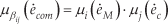
where $μ_{β_{i j}} ({\dot{e}}_{c o m})$ means the degree of the fuzzy set $β ({\dot{e}}_{c o m})$ fired by $μ_{i} ({\dot{e}}_{M})$ and $μ_{j} ({\dot{e}}_{c})$ . β is among the output fuzzy sets {NL, NM, NS, ZE, PS, PM, PL}.

Figure 4.

Block diagram of the proposed pre-compensation fuzzy logic control (PFLC) method

Table 2.

FAMM-1

	NL	NM	NS	ZE	PS	PM	PL
NL	NL	NL	NL	NL	NM	NS	ZE
NM	NL	NL	NL	NM	NS	ZE	PS
NS	NL	NL	NM	NS	ZE	PS	PM
ZE	NL	NM	NS	ZE	PS	PM	PL
PS	NM	NS	ZE	PS	PM	PL	PL
PM	NS	ZE	PS	PM	PL	PL	PL
PL	ZE	PS	PM	PL	PL	PL	PL

Table 3.

FAMM-2

	NL	NM	NS	ZE	PS	PM	PL
NL	PL	PL	PL	PL	PL	PM	PM
NM	PL	PL	PL	PM	PM	PS	PS
NS	PL	PL	PM	PS	ZE	NS	NM
ZE	PL	PM	PS	ZE	NS	NM	NL
PS	PM	PS	ZE	NS	NM	NL	NL
PM	NS	NS	NM	NM	NL	NL	NL
PL	NM	NM	NL	NL	NL	NL	NL

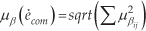
Evaluation of all the rules leads to

μ_{β} ({\dot{e}}_{c o m}) = s q r t (\sum μ_{β_{i j}}^{2})

(12)

The defuzzification strategy adopted is a simplified version of the ‘centre of gravity method’ as

{\dot{e}}_{c o m} = \frac{\sum (C_{β} . μ_{β})}{\sum μ_{β}}

(13)

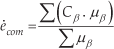
where C_β is the constant value for the fuzzy set β defined by the output membership function. The fuzzification, rule evaluation as well as defuzzification process for FIS_2 is the same as FIS_1. The surface view of output for FIS_1 and FIS_2 is shown in Figure 7.

Note that for the conventional fuzzy logic approach, there is only one fuzzy inference system that takes ė_c and e_c as inputs with the similar implementation as FIS_2. In order to conduct the comparison between PFLC and the conventional fuzzy logic approach, the same membership functions and implementations for the conventional fuzzy logic approach are adopted.

Figure 5.

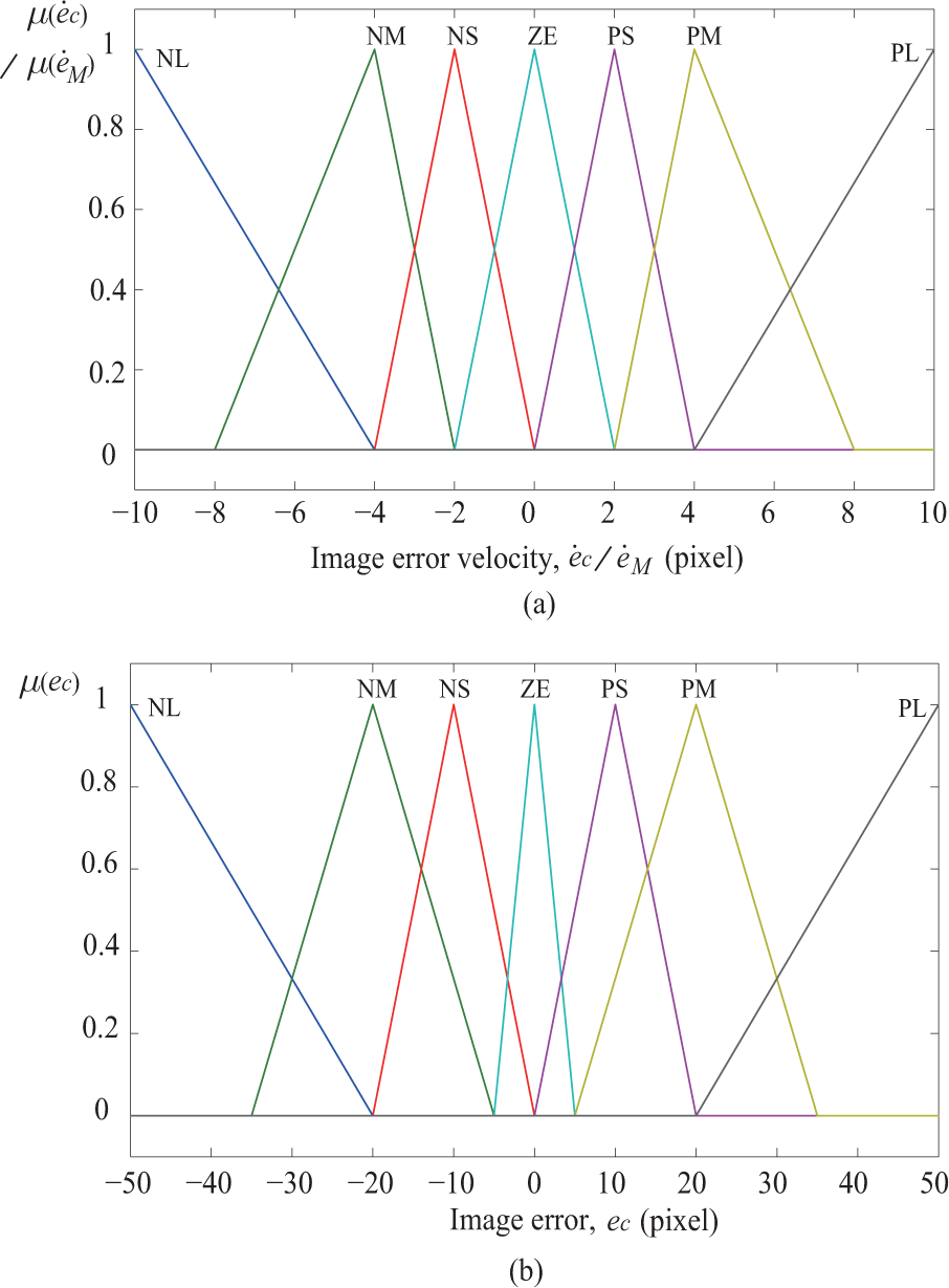
Membership functions for the input variables

4. Simulation study

In order to evaluate the analysis approach and to undertake a comparison, a numerical simulation is done using Matlab's fuzzy logic toolbox [22]. Evaluations of point-to-point regulation and high-speed vibration compensation have been conducted by using the simple cart model illustrated in Equations (1) – (10). The mass for main plant and compensation plant is set to be 28 kg and 2 kg respectively. Since we only conduct the horizontal motion, the variance of the image position for the system along the vertical direction is perceived as zero.

4.1 Point-to-point regulation

The start position and target position in image is set to be ξ _s = −200 and ξ _d = 0 respectively. From the start position, the entire system is controlled to move as a whole by the main plant's non-optimal controller, and here it is supposed to be a common PD controller. At the image position of ξ _r = −5, the compensation plant is activated to perform the relative motion under the conventional fuzzy logic control and the proposed PFLC method. As shown in Figure 8, the system shows a longer settling time if there was no compensation motion involved. Compared with the conventional fuzzy logic control, the proposed PFLC method shows improvement in suppressing the overshoot and reducing the settling time.

Figure 6.

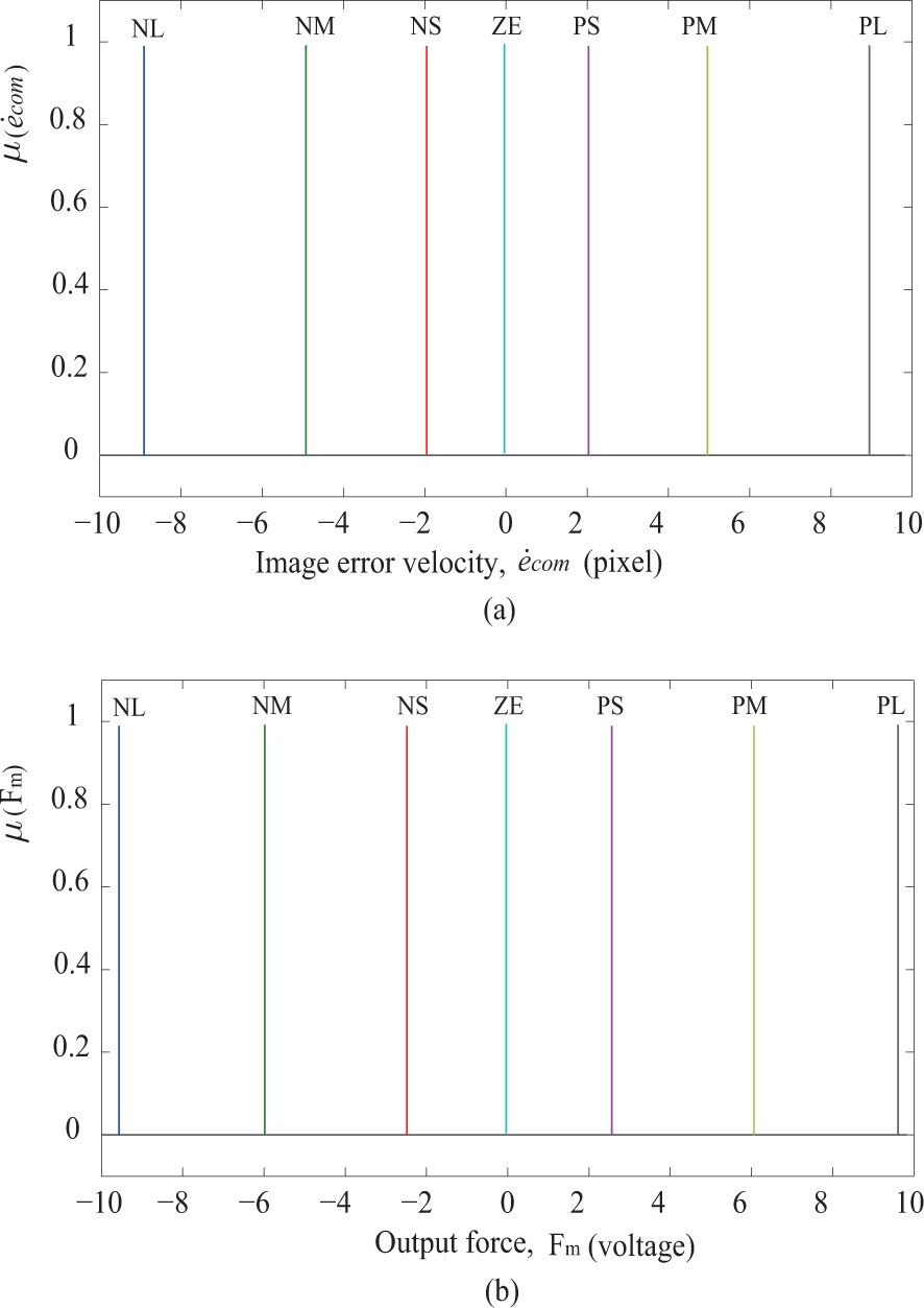
Membership functions for the output variables

4.2 Vibration compensation

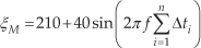
In order to check the system's compensation performance under high-speed motion, we make the main plant exhibit a sin (·) reciprocating motion and the feature point of the main plant in the images follow the pattern of:

ξ_{M} = 200 + 80 sin (2 π f \sum_{i = 1}^{n} Δ t_{i})

(14)

where f = 8 Hz represents the frequency and Δt_i =1 ms is the control cycle time. As will be shown later in the point-to-point experimental evaluation, the reason for choosing the frequency f = 8 Hz is that the main plant of the testbed has the oscillation frequency of 8 Hz while performing point-to-point positioning. Therefore, we choose f = 8 Hz as the evaluation frequency for vibration compensation. As shown in Figure 9, the reference trajectory represents the ideal trajectory of the regulation point where the vibration motion of the main plant can be exactly counteracted. It can be seen, both the conventional fuzzy logic method and the proposed PFLC method realized good compensation under the main plant's high-speed vibration motion. The compensation error is shown in Figure 10. It clearly shows that the proposed PFLC method had a smaller error than the traditional fuzzy control, and that was exactly the result of the pre-compensation from the feedback information of the main plant's motion. The applied force on the compensation plant is shown in Figure 11. It is quite interesting to see that the PFLC method actually applied a smaller force than the conventional fuzzy control method on average during the compensation process, which also tells the better efficiency of the proposed PFLC method.

Figure 7.

Surface view of the output for fuzzy inference. (a) : FIS_1; (b) : FIS_2

5. Experimental evaluations

In order to check whether the real system acts identically with the numerical simulation that has been conducted according to the model analysis, experimental evaluations on point-to-point regulation as well as the vibration compensation were conducted.

5.1 Point-to-point regulation

For the point-to-point regulation, firstly the whole system was regulated towards the target position in images by the main plant's rough PD controller from the start position ξ _s = −200 in images. The compensation plant's motion was triggered once the regulation point reached ξ _p = 0. During the experiment, for comparison, we simplified the regulation by letting ξ _p = ξ _d = 0. Thus once the compensation plant was triggered at the time t₀ = 2.15 s when it reached ξ _p , both the main plant and the compensation plant were regulated to stay at ξ_p. The results for three methods applied to the compensation plant are shown in Figure 12. It can be seen that the main plant of the testbed exhibited a 8 Hz oscillation before converging to the target position. The results show that compared with PD control and conventional fuzzy logic control, the proposed PFLC method reduced the image error during the whole regulation process. For the 10% error band, the settling time was reduced gradually from t_s4 to t_s3, t_s2 and t_s1, representing the point-to-point regulation without compensation, compensation under PD control, compensation under conventional fuzzy control and the proposed PFLC method respectively. The PFLC method had the smallest settling time for the same point-to-point regulation.

Figure 8.

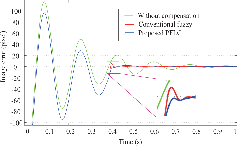
Simulation result of image error for point-to-point compensation

Figure 9.

Simulation result of image trajectory for vibration (8Hz) compensation

Figure 10.

Simulation result of image error for vibration (8Hz) compensation

Figure 11.

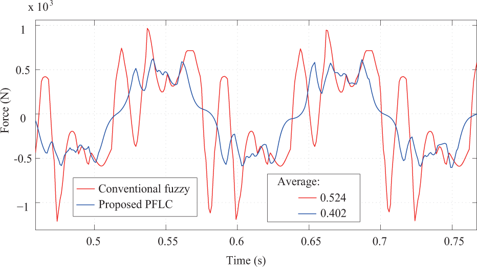
Simulation of stimulated force for vibration (8Hz) compensation

5.2 Vibration compensation

The same as the simulation above, a vibration compensation analysis was conducted to check how well the regulation point could keep aligned with the target position for different control methods while it was continually disturbed by the reciprocating motion of the main plant. Similarly to the simulation settings, we let the main plant follow a sin (·) reciprocating motion as

ξ_{M} = 210 + 40 sin (2 π f \sum_{i = 1}^{n} Δ t_{i})

(15)

and let the frequency f = 8 Hz, where Δt_i = 1 ms is the control cycle time. Three methods, namely the simple PD control, the conventional fuzzy logic control and the proposed PFLC method were adopted to conduct the comparison. Note that for the PD method, the gain coefficients have been tuned. For both the conventional fuzzy logic method and the proposed PFLC, few efforts were needed for parameter tuning and we tried to find the relatively good membership functions, especially for the output membership functions of FIS_1 and FIS_2.

As shown in Figure 13, the proposed PFLC method realized perfect compensation of the main plant's high-speed vibration motion, while the conventional fuzzy logic control had a less good performance and the PD method showed the worst. The compensation error is shown in Figure 14. This clearly shows that the proposed PFLC method had a smaller error than the other two methods. In another words, the regulation point could be regulated to the target point although it was constantly disturbed by the main plant's motion. Figure 15 shows the real-time information of the inputs and output of the FIS_1. It can be seen that during the ‘Active adjusting phase’, the compensation plant's motion ė_c had a major effect on the output of the FIS_1, while during the ‘Stable phase’, the main plant's motion ė_M had a major effect on the output ė_com. This implies the functioning of the pre-compensation term.

The applied force on the compensation plant is shown in Figure 16. This also illustrates the same phenomenon whereby the PFLC method actually applied a smaller force than the conventional fuzzy control method on average during the compensation process, which also can be perceived as the ‘passive advantage’ thanks to the pre-compensation. As for the PD method, it always tried to drive the compensation plant with the maximum force in order to realize the high-speed compensation, yet a phase delay constantly existed as shown in Figure 16 and Figure 13.

Figure 12.

Image error for point-to-point compensation

Figure 13.

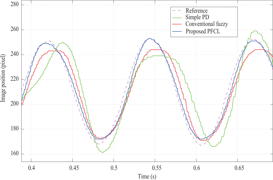
Image trajectory for vibration (8Hz) compensation

We also tried to realize the vibration compensation for several different motion speeds of the main plant. The results for a frequency of 4 Hz, 6 Hz and 8 Hz are shown in Figure 17 and 18, which illustrate the image error of different control methods. For the PD method, the image error basically becomes larger along with a higher motion speed of the main plant. The same trend can also be seen from the conventional fuzzy logic method except that the changing rate was small. For the proposed PFLC method, we could see that the image error almost kept the same range for different motion speeds of the main plant, all at comparatively low levels. The same phenomenon can be seen from the experiment evaluations on a random vibration test with the frequency ranging from 3 Hz to 8 Hz as shown in Figure 19. The video for vibration compensation with the proposed PFLC method can be found on the website [23].

6. Conclusions and future works

In this research, a model-independent pre-compensation fuzzy logic control algorithm has been proposed in order to realize the fine dynamic compensation control of the compensation plant in the context of 1-DOF DCRS. The DCRS has been adopted to realize motion regulations, such as positioning, at high-speed and with good accuracy. During this kind of regulation, the compensation plant for fine positioning is always dynamically disturbed by the main plant that is designated for the coarse positioning in a large work range. By analysing the motion of the 1-DOF DCRS with a simplified cart model, the pre-compensation portion is discovered, and by further combination with the fuzzy logic method, a cascade PFLC algorithm has been proposed without asking for the explicit mathematical models of the system. Both simulation and experimental evaluations show the consistent effectiveness of the proposed PFLC method. Compared with some control methods that involve the dynamic models to accomplish the high-speed and accurate motion regulation, the proposed PFLC method within the context of the DCRS is easy to implement and more flexible with regard to different application tasks.

Figure 14.

Image error for vibration (8Hz) compensation

Figure 15.

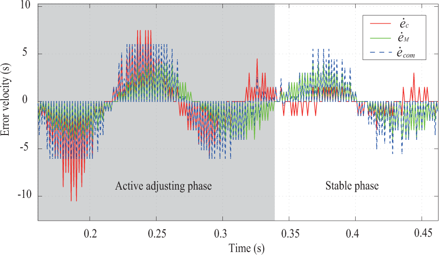
Inputs and output of FIS_1 for vibration (8Hz) compensation

Figure 16.

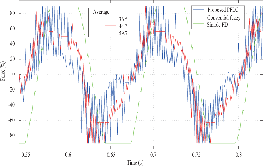
Output force for vibration (8Hz) compensation

Figure 17.

Image error for vibration (4Hz, 6Hz, 8Hz) compensation without pre-compensation

Figure 18.

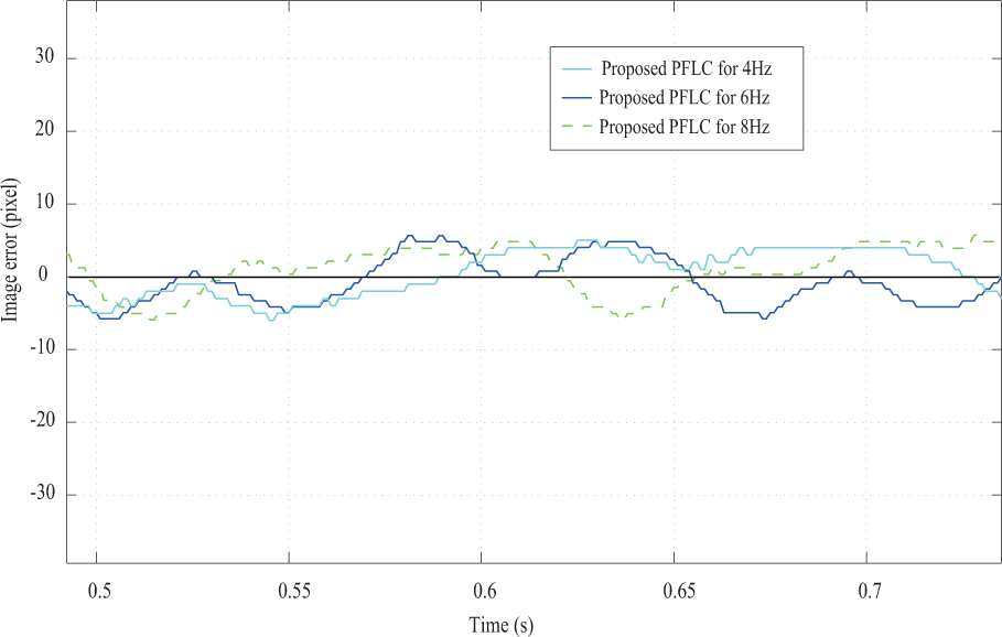
Image error for vibration (4Hz, 6Hz, 8Hz) compensation by PFLC

Figure 19.

Image error for random vibration compensation

Although the proposed approach has been illustrated for the 1-DOF DCRS in this paper, we think the proposed algorithm is extendible for DCRS with multiple DOFs. Since the proposed method is non-model-based and with good flexibility, we can basically assemble a multiple-DOF DCRS by using several 1-DOF DCRSs, and this is our future work.

References

Lewis

Dawson

Abdallah

(2003) Robot Manipulator Control: Theory and Practice. 2 Edition, New York: CRC Press.

Zhang

Gruver

Gao

(1999) Dynamic simplification of three degree of freedom manipulators with closed chains. Rob. Auton. Syst. 28: 261–269.

Zomaya

Morris

(1990) The dynamic performance of robot manipulators under different operating conditions. lEE Proc. on Control Theory and Applications. 137:281–289.

Yoshikawa

(1990) Foundations of robotics: Analysis and Control. Cambridge (MA): MIT Press.

Hogan

Sharon

Hardt

(1988) High bandwidth force regulation and inertia reduction using a macro/micro manipulator system. In: IEEE Int. Conf. on Robotics and Automation (ICRA). 1988 Apr 24–29; Philadelphia, PA USA. pp.126–132.

Sharon

Hogan

Hardt

(1993) The macro micro manipulator: An improved architecture for robot control. Robot. Comput.-Integr. Manuf. 10:209–222.

Lew

Trudnowski

(1996) Vibration control of a micro/macro-manipulator system. IEEE Control Systems. 16:26–31.

Kimata

Morita

Ukai

Kando

Matsuno

(2004) PDS control of macro-micro arm. In: IEEE Int. Workshop on Advanced Motion Control. 2004 Mar 28–28; Kawasaki, Japan. pp.123–128.

BaUhaus

Rock

(1992) End-Point Control of a Two-Link Flexible Robotic Manipulator with a Mini-Manipulator: Dynamic Coupling Issues. In: ASME Winter Annual Meeting. 1992 Nov 8–13; Anaheim, CA USA. pp.17–22.

10.

Stevens

How

(1996) The Limitations of Independent Controller Design for a Multiple-link Flexible Macro-Manipulator Carrying a Rigid Mini-Manipulator. In: 2nd ASCE Conf. on Robotics for Challenging Environments. 1996 Jun 1–6; Albuquerque, NM USA. pp.93–99.

11.

Hodac

Siegwart

(1998) Endpoint Control of a Fast and Precise Macro/Micro-Manipulator. In: 4th Int. Conf. on Motion and Vibration Control (MOV-IC). 1996 Aug 25–28; Zurich, Switzerland. pp. 883–888.

12.

Hodac

Siegwart

(1999) Decoupled macro/ micro-manipulator for fast and precise assembly operations: Design and experiments In: SPIE Conf. on Microrobotics and Microassembly. 1999 Sep 19–22; Boston, MA USA. pp.122–130.

13.

Yoshikawa

Hosoda

Doi

Murakami

(1994) Dynamic trajectory tracking control of flexible manipulator by macro-micro manipulator system. In: IEEE Int. Conf. on Robotics and Automation (ICRA). 1994 May 8–13; San Diego, CAUSA. pp. 1804–1809.

14.

Yang

Han

(2010) Dynamiccompensation control of flexible macro-micro manipulator systems. IEEE Trans. on Control systems technology. 18:143–151.

15.

Omari

Ming

Nakamura

Kanamori

Kajitani

(2000) Development of a High Precision Mounting Robot with Fine Motion Mechanism (2nd Report) – Control of the Fine Mechanism Considering Dynamic Response and Disturbance from Coarse Mechanism. The Japan Society for Precision Engineering. 66:1583–1589.

16.

Omari

Ming

Nakamura

Kanamori

Kajitani

(2001) Development of a High Precision Mounting Robot with Fine Motion Mechanism (3rd Report) – Control of the Fine Mechanism Considering Dynamic Response and Disturbance from Coarse Mechanism. The Japan Society for Precision Engineering. 67:1101–1107.

17.

Huang

Yamakawa

Senoo

Ishikawa

(2014) Dynamic Compensation by Fusing a High-speed Actuator and High-speed Visual Feedback with Its Application to Fast Peg-and-Hole Alignment, Advanced Robotics. 28:613–624.

18.

Lee

(1990) Fuzzy logic in control systems: Fuzzy logic controller – Part 1 and Part 2. IEEE Trans. Syst. Man Cybernet. 20:404–435.

19.

Ross

(2010) Fuzzy logic with engineering applications. 3rd edition, West Sussex: John Wiley & Sons Ltd.

20.

Kim

Lee

Kim

(1993) Fuzzy precompensation of PID controllers. In: IEEE conf. on Control Applications.1993 Sep 13–16; BC, Canada. pp. 183–188.

21.

Alavandar

Jain

Nigam

(2009) Bacterial foraging optimized hybrid fuzzy precompensated PD control of two link rigid flexible manipulator. Int. J. of Computational Intelligence Systems. 2:51–59.

22.

The MathWorks Inc (2014) Fuzzy logic toolbox user's guide. Available from: http://www.math-works.co.jp/help/pdf_doc/fuzzy/fuzzy.pdf. Accessed on 15 May 2014.

23.

Dynamic compensation for random vibration with PFLC algorithm. Available from: http://www.k2.t.u-tokyo.ac.jp/fusion/DynamicCompensation. Accessed on 04 May 2014.

	NL	NM	NS	ZE	PS	PM	PL
NL	NL	NL	NL	NL	NM	NS	ZE
NM	NL	NL	NL	NM	NS	ZE	PS
NS	NL	NL	NM	NS	ZE	PS	PM
ZE	NL	NM	NS	ZE	PS	PM	PL
PS	NM	NS	ZE	PS	PM	PL	PL
PM	NS	ZE	PS	PM	PL	PL	PL
PL	ZE	PS	PM	PL	PL	PL	PL

	NL	NM	NS	ZE	PS	PM	PL
NL	PL	PL	PL	PL	PL	PM	PM
NM	PL	PL	PL	PM	PM	PS	PS
NS	PL	PL	PM	PS	ZE	NS	NM
ZE	PL	PM	PS	ZE	NS	NM	NL
PS	PM	PS	ZE	NS	NM	NL	NL
PM	NS	NS	NM	NM	NL	NL	NL
PL	NM	NM	NL	NL	NL	NL	NL

	NL	NM	NS	ZE	PS	PM	PL
NL	NL	NL	NL	NL	NM	NS	ZE
NM	NL	NL	NL	NM	NS	ZE	PS
NS	NL	NL	NM	NS	ZE	PS	PM
ZE	NL	NM	NS	ZE	PS	PM	PL
PS	NM	NS	ZE	PS	PM	PL	PL
PM	NS	ZE	PS	PM	PL	PL	PL
PL	ZE	PS	PM	PL	PL	PL	PL

	NL	NM	NS	ZE	PS	PM	PL
NL	PL	PL	PL	PL	PL	PM	PM
NM	PL	PL	PL	PM	PM	PS	PS
NS	PL	PL	PM	PS	ZE	NS	NM
ZE	PL	PM	PS	ZE	NS	NM	NL
PS	PM	PS	ZE	NS	NM	NL	NL
PM	NS	NS	NM	NM	NL	NL	NL
PL	NM	NM	NL	NL	NL	NL	NL

A Pre-Compensation Fuzzy Logic Algorithm Designed for the Dynamic Compensation Robotic System