Sage Journals: Discover world-class research

Abstract

To obtain accurate information about the interested physical phenomenon, many nodes should be deployed and collaborated to extract data about the event source. This article proposes a Low Power Self Scheduling protocol for mobile point source reconstruction. The motivation is clear, to provide high level QoS (reconstruction distortion) and reduce energy consumption. This article first obtains a distance to the event source, in which all sensing reports are collected to minimize the reconstruction distortion. This distance is relatively constant under different network densities. Then the mobility of the event source is considered. Sensor nodes are self-scheduled to join or leave the representative nodes group, which guarantee that those appropriate nodes will always be the group member. Simulation validates the effectiveness of the presented scheme.

Keywords

Energy Efficient Reconstruction Distortion Point Source Mobility Sensor Networks

1. Introduction

Sensor networks are generally comprised of densely deployed sensor nodes collaboratively observing and communicating information about physical phenomenon. Dense deployment of sensor nodes makes the sensor observations highly correlated in the space domain. Obviously, it is important to design energy-efficient communication protocols to exploit the potential advantages of spatial correlation.

Considerable research efforts have been addressed on the correlation issues [e.g., 1–12]. In ref. [1–5], different coding models, optimal network density, and transmission structure are applied to exploit the spatial correlation in sensor networks. Reference [6] derived a lower bound on the best achieved end-to-end distortion for different coding schemes. References [7–9] proposed different approaches to collect only a small part of the observation samples, so as to minimize or even eliminate the possible shared channel contention.

In our previous work [10, 11], we argued that the distance first method can significantly reduce the reconstruction distortion with fewer node observation samples, which select the representative nodes by the order of the distance to the event spot. However, several components in [10] and [11] are chosen in an empirical manner, which need further investigation. The idea behind [10] and [11] is consistent with the conclusions of [12]. Reference [12] also stated that the distance first selection assumes that the location of the event source is known. But in our opinion, the absolute coordinate is unnecessary. Through numerical simulation, we find out that there exists a range to the event source within which all the sensing reports should be collected to minimize the reconstruction distortion. The results validate our intuition and serve as a guideline to the design of communication protocol.

In the real world, the physical event may be mobile, so the communication protocols should be designed to support mobility and allow the user to track the mobile event continuously in an energy-efficient way. Unfortunately, none of the above work [7–11] take this impact into consideration. This article addresses the sensor collaboration issue of mobile source reconstruction while filtering out the spatial correlation among the sensing reports. To the best of our knowledge, this is the first research effort that joins these two aspects (event mobility and spatial correlation) together. Under our introduced LPSS scheme, sensor nodes are self-scheduled to join or leave the representative group which guarantees that those appropriate nodes will always be the group member to improve the accuracy of reconstruction. The proposed protocol is highly scalable, since no global information is assumed at individual sensor nodes.

The rest of the article is organized as follows. In Section 2, we discuss some related work to place our contributions in context. Section 3 provides the theoretic foundation and the underlying idea of our proposed scheme. Next, in Section 4, we propose the LPSS protocol, and the simulation results are presented in Section 5. Section 6 provides the concluding comments.

2. Related Works

Taking advantage of the spatial correlation can be conducted at the MAC layer, and several protocols have been introduced. In ref. [7] and [8], Jamieson et al. tried to minimize the time taken to send R (less than N) messages without collision when N nodes sensed an event and contended for transmitting on a shared channel simultaneously. And the remaining N - R potential transmitter suppress their message once R has been sent. The proposed mechanism is named Sift. Ref. [9] divided the network into sub-parts, in which only one node was allowed to deliver records. The so-called CC-MAC protocol itself consists of two components: the Event MAC (E-MAC), which filters sensor node measurements to reduce traffic and the Network MAC (N-MAC), which forwards the filtered measurements to the sensor network sink. The QS-Sift and HS-Sift protocols in our prior work 10 and 11 was designed to further conserve energy by taking the sensing report quality into consideration.

Although our work is not for target tracking, but the tracking mechanism can be helpful in the mobile source reconstructing. Ref. [13] addressed the tracking problem by taking into account both the coverage and the quality of monitoring (QoM). Ref. [13] argued that for a reasonably dense sensor network, QoM can be met with high probability if we track the target with the use of the closest sensor. Zhang et al. [14] and [15] formalized the tracking problem as a dynamic convoy-tree reconfiguration process and introduced an optimized complete and an interception-based reconfiguration schemes. The idea of the LPSS protocol is originated from the predicted-based scheme for dynamic tree expansion and pruning in [14] and [15].

From the signal processing perspective, reconstructing a signal field using data samples is a classical problem, and the literature is extensive [e.g., [16–17]]. Dong et al. [16] analyze the impact of data retrieval on the reconstruction performance. They connect the data retrieval protocol and different sampling schemes, and their research shows that the deterministic and random pattern performs differently in different SNR regimes. Zhao et al. [17] propose a so-called QUIRE protocol to optimize the network performance by partitioning the sensor networks into a disjointed and an equal-sized cell, and the cell size is chosen to minimize the number of transmissions required to a given QoS by exploiting the spatial correlation of the signal field.

The difference between this article and the above research is that target tracking neglects the relation among data samples and [16–17] does not consider the case of the mobile source, while we join these two aspects together.

3. Problem Statements

3.1. Sensor Deploying Model

Consider a large number of sensor nodes uniformly and randomly deployed over the surveillance region, where L_i denotes the location coordinates of node i. To save energy, the nodes sleep most of the time. As long as the number of nodes is large, the node distribution can be modeled as a homogeneous Poisson process with node density λ [13]. That is, given an area of the size | A | in the field, the number of nodes in the area, μ( A ), follows the Poisson distribution with parameter λ| A |, i.e.,

Prob (μ (A) = m) = e^{- λ | A |} \frac{(λ | A |)^{m}}{m!}, m = 0, 1, \dots, \infty

We also assume that each sensor node has the capability to gather its own location information via, for example, GPS or other techniques such as triangulation.

3.2. Point Source Model

In this article, we focus on the point source model only, and leave the field source scenario (both defined in [12]) in future work. A point source is assumed to generate a continuous signal which can be modeled by a Gaussian random process. The point source is supposed to be moving in the surveillance region. For ease of illustration, we assume that the coordinate axis is centered at the point source.

We also assume that the signal strength (i.e., the energy) of the received signal decreases exponentially with the propagation distance [12, 13].

r_{i} = a \cdot ∥ x_{i} ∥^{- α} + ω_{i},

(1)

where r_i is the received signal strength in the i^th sensor, ɑ ∈ ℜ is the (unknown) strength of the signal from the point source, x_i ∈ ℜ² is the known position of the i^th sensor, α is the (known) attenuation coefficient, and ω _i is the white Gaussian noise with zero-mean and variance σ².

Each node i send back a scaled version of the observed sample

y_{i} = ∥ x_{i} ∥^{α} r_{i}

based on its distance to the event source. The sensed and estimated signal of each node is shown in Fig. 1, where the nodes are numbered by the distance and the axis Y is based on the logarithmic scale.

Figure 1.

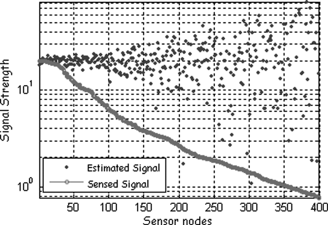
Signal attenuation and the corresponding estimation (400 nodes in a region of 5 by 5, and a = 20).

It is clear from Fig. 1 that the estimation error increases with the distance to the source. Take the scenario of Fig. 1 for example, by using the theory of probability, it is easy to know that when lying 4 units away from the source, the ratio of the nodes whose error is smaller than 10% is only 9.56%, 15.86% for those with 3 units, 31.08% for those with 2 units, compared with 68.26% for those with 1 unit. In fact, the nodes estimation whose number is larger than 100 is nearly unusable.

3.3. Source Reconstruction Distortion

In many sensor networks applications such as target or fire detection, we are interested in estimating the signal generated by the event source using node observations. Under a specific MAC scheme, after some collection time, the sink node receives a total of M packets originating from some M points. In other words, the sink node obtains the M noisy sample. The event source can be simply computed by taking the average of all reports received at the sink. It is reasonable [18] to argue that the global estimator should weight the estimation of each sensor appropriately since the sensor closer to the source produces more reliable decisions. And the confidence in each sensor decision is proportional to the strength of the signal (the SNR) at the sensor location. Hence, S', the estimate of the source S, is a weighted average of all the event information received at the sink

S^{'} = \sum_{i = 1}^{M} ω_{i} y_{i}

where

ω_{i} = s n r_{i} / \sum_{i = 1}^{M} s n r_{i .}

The distortion achieved to estimate the event S is then given by

D_{E} = E [(S - S^{'})^{2}]

The reconstruction distortion achieved using ordered selection (named after [12] which are actually the same as the distance first method in [10] and [11]) and the random selection is shown in Fig. 2. For random access, the nodes in the sensing region are chosen randomly to send information. On the contrary, for ordered selection, the closest M nodes to the event, are chosen to transmit data. The higher value of M corresponds to the nodes farther away from the event being chosen.

Figure 2.

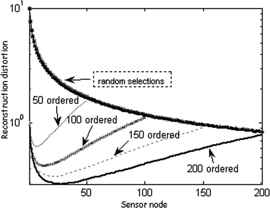
Average distortion achieved by ordered and random selection schemes (50, 100, 150, 200 nodes in a region of 5 by 5, respectively, and a = 20).

It is clear from Fig. 2 that the reconstruction distortion does not always fall with the increase of the collected data samples under the ordered selection scheme. After a certain number of nodes have been selected, the achieved distortion will increase instead. This is caused by the fact that the farther observation reports will also bring in more observation error. In general, the nodes farther than a certain range shall not send data at all. In other words, there exists an optimal value of the number of representative nodes (nodes which need send their monitored information back to the sink). At the same time, we notice that the optimal value varies with the network density, while the random selection method nearly does not seem to have been influenced.

3.4. Basic Ideas

As we have discussed, the ordered selection scheme can significantly reduce the reconstruction distortion even with fewer observation samples. Now our attention is to focus on how to obtain the optimal value of the representative nodes. Unfortunately, the network density varies throughout the network lifetime because some sensor nodes will die of energy depletion, some will be reinforced, and some may go to sleep for power saving. Consequently, the exact optimal value will keep varying as well. Besides, the calculation of the optimal value may need centralized processing which is unfit for the sensor networks.

By observing Fig. 2, we get to know that the optimal value increases with the network density, which prompts us to switch our focus to the ranges, because when the area is fixed, the number of nodes will increase with the density. Will the corresponding distance to the event source (i.e., the area of the representative node region) keep constant? In order to gain more insight regarding this aspect, we deploy 25 to 450 sensor nodes randomly in a 5 × 5 to 25 × 25 grid to produce different network densities. The average optimal distance (corresponding to the optimal representative nodes number) of 10,000 trials using ordered selection is shown in Fig. 3. The mean value and the variance of the optimal distance are plotted in Fig. 4.

Figure 3.

Average optimal distance of different network density.

Figure 4.

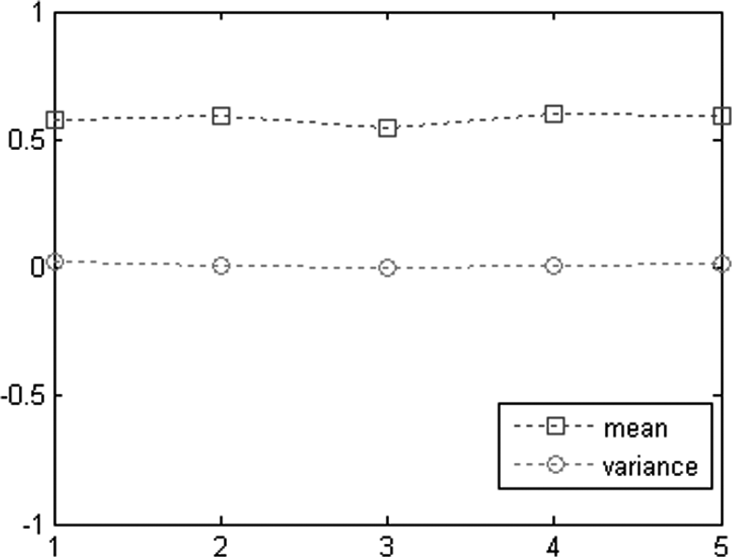
Mean value and variance of the 5 different network range cases of Fig. 3.

The above two results validate our assumption, the optimal distance stays relatively constant under different network densities. The variance in Fig. 4 is close to zero, which means the optimal distance is very stable. This characteristic can be simply explained as follows, because of the exponential attenuation of the event signal, once beyond a certain threshold, the sensed signal will be buried by the background noise, and this behavior has no relation to the network density.

4. LPSS Design

4.1. Optimal Distance Calculating

According to the results obtained in the last section, we introduce an Iterative Distance Calculating (IDC) algorithm to compute the optimal distance such that the minimal distortion can be obtained. Based on the IDC algorithm results, the LPSS is performed distributively by each sensor node to achieve the required performance. The IDC algorithm requires only the statistical properties of the node distribution as input and provides the ideal distance to the event source as output. Based on the statistical properties, the IDC algorithm first forms a sample topology. Then, as shown in Fig. 5, the algorithm starts with the minimal distance and iteratively increases the distance to the event source, r, until the reconstruction distortion ceases falling. For each value of r, the distortion D_E is calculated. When the IDC algorithm converges, the optimal distance is informed to all sensor nodes.

Figure 5.

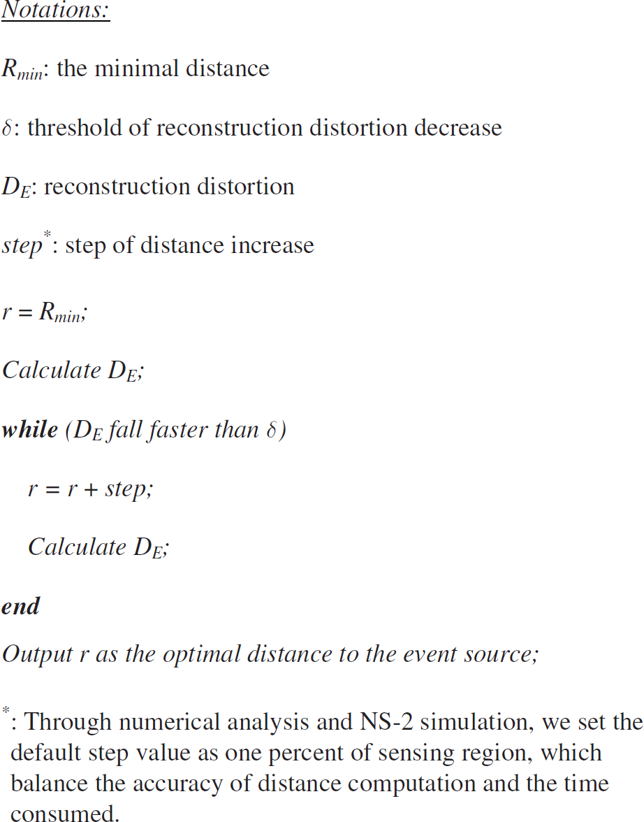
Iterative distance calculating algorithm.

4.2. Source Distance Estimation

Instead of solving for the unknowns in Eq. (1) based on energy reading from multiple sensors, we use the following simple approximating approach. The distance from the event to a sensor, say node i, can be estimated (with the noise ignored and the conjectured signal strength from the event) as

d = (r / a)^{- 1 / α} .

That is, the possible position at which the event may be located is a circle centered at node i with radius d. Note that initially a is set to a default value and dynamically adjusted according to the previous reconstruction results. The performance of this simple method is verified in the next section through simulations.

4.3. Source Motion Prediction

In this section, we study the impact of mobility on the source estimation. For ease of analysis, we assume that the event follows the modified random waypoint model [19]. However, we claim that our proposed scheme and the analysis methodology can be applied to other mobility models. Specifically, in the modified random waypoint model, a node randomly chooses a destination point in the area and moves at a random chosen non-zero minimum speed toward it. After the node arrives at the destination point, it pauses for a random time, chooses a new destination and moves toward that destination.

Our idea can be illustrated in Fig. 6. At time t, the event will arrive at P_t from location P_t-1. And the optimal sensing region (a circle center at the event source whose radius equals the optimal distance r) will also switch from Disk_t-1 to Disk_t. Obviously, the sensor node lying region ① will be too far-away to the event immediately and shall turn to sleep. Region ③ is the area where the sensor nodes need to wake up because the event will soon be close enough, and the nodes in region ② shall hold their state because their distance is still nearer than the optimal range.

Figure 6.

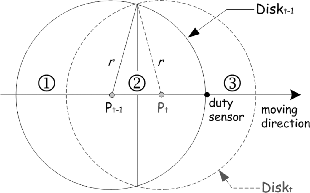
Event source mobility prediction.: Notations: r: optimal distance; d: distance to the event of duty sensor at time t; P_t: event location at time t.

The proposed scheme operates as follows: After a sensor node has detected an event, it continuously monitors the source movement for a while and determines the moving direction of the source based on the angles-of-arrival of consecutive measurements [13]. With the knowledge of the moving direction and the distance to the event, a sensor node (duty sensor in Fig. 6) which finds the event move directly toward itself and its distance equals the optimal value will broadcast a short relay message that includes

the location P_t-1 and

the location Pt.

On receiving the relay message, node i checks if it has received the message before. If so, the message is ignored. Otherwise, it will compute its distance to the position P_t-1, d(L_i, P_t-1) and Pt, d(L_i, P_t). If d(L_i, P_t-1) ≥ r and d(L_i, P_t) ≤ r are satisfied, then it will have to turn on its radio (such as the nodes in region). Once a sensor node is aware that the event source is out of the optimal range, it will switch off its radio and turn to sleep (such as the nodes in region ①).

There still exists a problem that nodes outside the optimal sensing region are sleeping, so they will not be able to receive the broadcasted relay message. To address this, the RFID impulse method [20] can be used to wake them up. The relay message is broadcasted on a RFID radio. Once a node receives the message, it will check if the above conditions are satisfied. The node will turn on its radio and retransmit the relay message if the conditions are satisfied, otherwise it will just ignore the message and keep on sleeping.

In the above scheme we do not consider the (rare) case that right after the duty sensor broadcast the relay message, the event changes its direction and moves towards some other place. This case is shown in Fig. 7, and the red dash-dot and the blue dashed circle are the actual and the predicted optimal sensing region respectively. To deal with this case, we have to choose a new duty sensor to waken nodes which d(L_i, P_t-1) ≥ r and d(L_i, P_t') ≤ r are satisfied, i.e., nodes lie outside the Disk_t-1 and inside Disk_t' (the actual optimal sensing region). And the new duty sensor will broadcast a relay-update message that includes

the location P_t-1 and

the new location Pt'.

Figure 7.

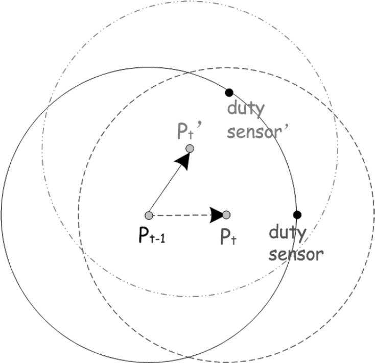
Event source mobility prediction.: Notations: P_t': actual event location at time t; P_t: predicted event location at time t.

In the above discussion, we claim that the duty sensor is the one which finds the event to move directly toward and whose distance equals the optimal value. But in practice, there may be many nodes which will declare themselves as the duty sensor at the same time because of the high network density or, on the contrary, no single node can play this role just because the network is too sparse. There are two ways of dealing with this case. First, a delay based competition algorithm is applied. Every node which finds the event source moving closer will broadcast, after a weighted delay, the relay message expressing its willingness to be a duty sensor. The weight is inversely proportional to the distance to the source and the angle θ of the source direction to itself (Fig. 8). Hence, the node whose angle equals π and distance equals r will broadcast the relay message first. If a sensor receives a relay message from some other nodes before its own broadcast it will suppress its own broadcast and will not be a duty sensor. Once a sensor broadcasts the message, it will become a duty sensor.

Figure 8.

Angle of source direction.

With the weighted delay mechanism, it is also possible that there exist multiple duty sensors at the same time. This is caused by the moving direction measurement error, or its own relay message of one node has been transmitted before the other transmitted relay message has been received. If these cases happen, a node will be associated with more than one duty sensor whose estimation could be different. We use a simple solution to address this problem. If a node receives several RFID relay messages, only the first arrived one will be processed. The contained location information is used to judge if it has to wake up, and the relay message that arrived later is just dropped.

5. Simulations

5.1. Accuracy of the Distance Estimation Method

It is obvious from the above discussion that the performance of LPSS depends on the accuracy of the distance estimation. The effectiveness of the estimation algorithm is verified by numerical simulation using Matlab. Let 100 sensor nodes be randomly distributed in a 10 × 10 m square region, and the event source is placed on a corner of the region. The simulation results are averaged over 10000 runs.

Figure 9 illustrates the numeric results of the distance estimation, in which the sensor nodes are numbered by the distance to the event. From the figure, we get to know that the estimating method performs very well for nodes surrounding the event source (less than 2 units), and the performance begins to drop since then (especially for those beyond about 5 units). This result is consistent with the Fig. 1, because the signal attenuate is exponentially characteristic. When being far enough, the sensed signal is very close to zero. But the poor estimation performance of the farther nodes does not matter because we are only interested in the nodes lying in the limited optimal range.

Figure 9.

Distance estimation.

5.2. Network Simulation Environment

Simulation is performed in a 50 × 50 m² square region where 400 nodes are randomly distributed. The event source is also randomly generated in the square. The nodes are modeled according to the NS-2 wireless nodes module and the energy model. The transmission range of each node is 30 m with an average energy consumption of 24.75 mW, 13.5 mW, and 15 uW during transmitting, receiving, and sleeping respectively. We assume that the nodes consume the same energy for idling listening, as well as for receiving.

The different traffic load is produced by varying the collection and reporting the interval of each node, which is used to investigate the performance of our scheme. Each simulation is performed for 600 s. Without loss of generality, we simulate the event source mobility as follows: the event source velocity is randomly chosen in [1, 10] m/s, and the direction is a random variable uniformly distributed in [0, 2π). The mobility direction is independently updated in 0.5 s, while the generator guarantees that the event source would not move out of the surveillance region in the next time period of 0.5 s.

5.3. Effectiveness of LPSS

The achieved reconstruction distortion for the static point source is shown in Fig. 10. Figure 10 reveals that LPSS achieves much lower distortion (about 34%) at the sink node than CC-MAC, which follows from the fact that the sensing quality is taken into consideration in the process of filtering out the spatial correlation. Hence the ratio of the accurate event reports gathered is much higher than that of CC-MAC when the same number of the representative nodes are selected. The performance of LPSS, HS-Sift, and QS-Sift is very close because all three mechanisms have taken advantage of the sensing quality.

Figure 10.

Comparison of distortion achieved for static point source.

As shown in Fig. 11, the reconstruction distortion of CC-MAC, QS-Sift, and HS-Sift increase fast when the source mobility is concerned. The result shows that these protocols cannot track the mobile event precisely, because sensing reports of poor quality are collected when the event source moves. However, the LPSS perform very well when compared with the other three schemes, which is what we have expected. This advantage is due to the motion prediction and waking-up the sleeping nodes mechanisms of LPSS.

Figure 11.

Comparison of distortion achieved for mobile point source.

The cost of LPSS to achieve such performance improvement is shown in Fig. 12 and Fig. 13. It is easy to know from Fig. 12 that the average energy consumption of LPSS, QS-Sift, and HS-Sift are close when applied for the static point source. They all have the significant energy conservation compared with S-MAC with the help of spatial correlation-based approach. The proposed LPSS also consumes about 49% less energy compared with CC-MAC due to the better quality of sensing data collected.

Figure 12.

Comparison of average energy consumption for different schemes in static point source.

Figure 13.

Comparison of average energy consumption for different schemes in mobile point source.

When the point source is mobile, the average energy consumption is displayed in Fig. 13. Some nodes will become very far from the source when the event source moves away. Hence a large amount of energy is wasted because they keep sensing and transmitting. The average energy consumption of CC-MAC, QS-Sift, and HS-Sift increase fast as shown in Fig. 13. On the contrary, the LPSS still maintains its energy-efficient characteristic due to the motion prediction mechanism.

6. Conclusions

In this article, we propose a LPSS protocol for mobile point source reconstruction in event-driven sensor networks. This article finds out that there exists an optimal distance to the event source within which all the sensing reports should be collected to minimize the reconstruction distortion. The distance is constant under different network densities. LPSS adaptively schedule sensor nodes to join or leave the sensing group which guarantee only those most appropriate nodes will always be in the sensing group. Simulations are conducted to verify the effectiveness of the proposed scheme.

References

Bandyopadhyay

Coyle

E. J.

, “Spatio-temporal sampling rates and energy efficiency in wireless sensor networks,” in Proc. of the 23rd IEEE INFOCOM, 2004.

Cristescu

Beferull-Lozano

Vetterli

, “On network correlated data gathering,” in Proc. of the 23rd IEEE INFOCOM, 2004.

Cristescu

Beferull-Lozano

, “Lossy network correlated data gathering with high-resolution coding,” in Proc. of the 4th Int'l Symposium Info. Processing in Sensor Networks (IPSN′05), 2005.

Cristescu

Vetterli

, “On the optimal density for real-time data gathering of spatio-temporal processes in sensor networks,” in Proc. of the 4th Int'l Symposium Info. Processing in Sensor Networks (IPSN′05), 2005.

Ganesan

Cristescu

Beferull-Lozano

, “Power-efficient sensor placement and transmission structure for data gathering under distortion constraints,” in Proc. of the 3rd Int'l Symposium Info. Processing in Sensor Networks (IPSN′04), 2004.

Gastpar

Vetterli

, “Power, spatio-temporal bandwidth, and distortion in large sensor networks,” IEEE J. on Selected Areas in Commun, vol. 23, no. 4, pp. 745–754, 2005.

Tay

Y. C.

Jamieson

Balakrishnan

, “Collision-minimizing CSMA and its applications to wireless sensor networks”, IEEE J. on Selected Areas in Commun, vol. 22, no. 6, pp. 1048–1057, 2004.

Jamieson

Balakrishnan

Tay

, “Sift: A MAC protocol for event-driven wireless sensor networks,” in Proc. of 3rd European Workshop on Wireless Sensor Networks (EWSN′06), 2006.

Vuran

M. C.

Akyildiz

I. F.

, “Spatial Correlation-based Collaborative Medium Access Control in Wireless Sensor Networks,” IEEE/ACM Trans. Networking, vol. 14, no. 2, pp. 316–329, 2006.

10.

Zhao

Chen

Z. G.

Zhang

L. M.

G. H.

, “HS-sift: hybrid spatial correlation-based medium access control for event-driven sensor networks,” IET Communications, vol. 1, no. 6, pp. 1126–1132, 2007.

11.

Zhao

Chen

Z. G.

Z. H.

, “QS-sift: QoS and spatial correlation-based medium access control in wireless sensor networks”, Int'l J. Sensor Networks, vol. 2, no. 3/4, pp. 228–234, 2007.

12.

Vuran

M. C.

Akan

O. B.

, “Spatio-temporal characteristics of point and field sources in wireless sensor networks,” in Proc. of IEEE Int'l Conf. Commun.(ICC′06), 2006.

13.

G. H.

Hou

J. C.

, “Tracking Target with Quality in Wireless Sensor Networks,” in Proc. of IEEE Int'l Conf. Network Protocols (ICNP005), 2005.

14.

Zhang

W. S.

Cao

G. H.

, “Optimizing tree reconfiguration for mobile target tracking in sensor networks,” in Proc. of the 23rd IEEE INFOCOM, 2004.

15.

Zhang

Cao

, “DCTC: dynamic convoy tree-based collaboration for target tracking in sensor networks,” IEEE Trans. Wireless Communication, vol. 3, no. 5, pp. 1689–1701, 2004.

16.

Dong

Tong

Salder

B. M.

, “Impact of data retrieval pattern on homogeneous signal field reconstruction in dense sensor networks,” IEEE Trans. Signal Processing, vol. 54, no. 11, pp. 4352–4364, 2006.

17.

Zhao

Tong

, “Energy-efficient information retrieval for correlated source reconstruction in sensor networks,” IEEE Trans. Wireless Communication, vol. 6, no. 1, pp. 157–165, 2007.

18.

Song

Y. C.

Tong

Swami

, “Asymptotic Locally Optimal Detector for Large-Scale Sensor Network under the Poisson Regime,” IEEE Trans. on Signal Processing, vol. 53, no. 6, pp. 2005–2017, 2005.

19.

Yoon

Liu

Noble

, “Random waypoint considered harmful,” in Proc. of the 22nd IEEE INFOCOM, 2003.

20.

Ruzzelli

A. G.

Jurdak

O'Hare

G. M. P.

“On the RFID wake-up impulse for multi-hop sensor networks,” in Proc. of the 5th ACM Conf. on Embedded Networked Sensor Systems (SenSys′07), 2007.

Optimizing Energy-Efficient Reconstruction of Mobile Point Source in Sensor Networks

Abstract

Keywords

1. Introduction

2. Related Works

3. Problem Statements

3.1. Sensor Deploying Model

3.2. Point Source Model

4.1. Optimal Distance Calculating

4.3. Source Motion Prediction

5.1. Accuracy of the Distance Estimation Method

5.3. Effectiveness of LPSS

References