
Abstract
Most object tracking techniques find the exact locations of an object, while many other applications are only interested in the object's path rather than its locations. This provides an opportunity to reduce the existing tracking methods' resource usage by only focusing on the path detection. Taking advantage of this opportunity, this article presents two new minimalist approaches for accurately detecting unknown available passages in a sensor field without requiring the exact locations of the objects. In the first approach, each sensor sends its own location to a base station when it senses an object of interest. The base station uses b-spline curves to build the object's path online. Since each sensor sends its location data just once per new path, the first approach is a minimalist approach. The second approach is offline and uses non-uniform rational b-spline (NURBS) curves. Since NURBS needs weighted locations, each sensor sends its own location in addition to the number of times it has sensed an object based on the object's weight. Using the same simulation models, both approaches greatly reduce power consumption and improve the accuracy of the computed paths. The NURBS approach has proved to be robust on false alarms and improves the accuracy of path detection up to 95 percent, which is very close to detecting the object's actual path.
Introduction
The novelty of smart environments has partly been realized today by using small-scale wireless sensor networks. As technology grows, each sensor gets smaller in size and price and stronger in capabilities and battery life, making it more feasible for everyday usage. With cheaper but more powerful sensors, many new practical applications can be developed, including habitat monitoring, environmental monitoring, and battlefield surveillance.
Object tracking is a well-known field in wireless sensor networks (WSN) technology. Object tracking determines the location of an object (or multiple objects) in a physical area. An extension to object tracking is target tracking, which deals with targeting a moving object. There are many approaches and algorithms in the field of entity tracking today [1] that are used to localize an object in the field and monitor its movement in a network using sensory data, so pursuers can predict where the opponent is going. These approaches differ, though, in attributes like low energy consumption [2], accuracy, real-time tracking, and scalability [3].
Another significant problem related to object tracking is robot navigation [4]. Here, the main concern is not the location of a moving object but the discovery of a path in an unknown physical area. Existing approaches use sensory data from sensors to navigate a robot that avoids obstacles along a path. The pursuer-evader game is another example that requires a similar type of robot navigation [1]. It uses sensory data to tell a pursuing object where to chase an evading object. In both problems, neither robots nor pursuers have any information about their target's location of their targets. A WSN system deployed in the field uses sensory data to find the targets and lead objects to them along safe paths (avoiding physical or opponent obstacles).
In many cases, pursuers are neither interested in the locations of objects nor in finding new paths along which to lead robots. Instead, they are interested in finding existing paths in unknown harsh, dangerous fields. There may be safe paths in these fields that the opponents use but the pursuers are unaware of. WSNs can be deployed in such fields to detect existing unknown paths by monitoring the movement of the objects using the paths. This is useful for many applications. For example, in habitat monitoring, we can discover the routes animals use for migration, or we can find the passageways used by animals in a jungle. In battlefield surveillance, there are frequently hidden areas with passages that only the enemy knows about, which they use to prevent others from advancing. By deploying WSNs, pursuers can find these safe passages when enemy objects cross the field.
In this article, we present two new approaches to detect unknown available passages in a sensory field. Contrary to existing object tracking methods that try to find the exact locations of objects, our proposed approaches only focus on finding an object's paths. Both approaches use minimal sensory data and spline curves. The first approach is online and uses b-spline curves; the second approach is offline and uses non-uniform rational b-spline (NURBS) curves to improve path detection accuracy.
The article is organized as follows: The next section takes a brief look at related work in the area of object tracking. Sections 3 and 4 discuss the problem of path detection. Section 5 presents new approaches to path detection. Section 6 reports our simulation results, and Section 7 concludes the article.
Related Work
There is a great deal of literature available on object tracking problems that use filters for classification. Some other methods, like probabilistically tracking multiple objects in an efficient manner, have also been studied [1]. We briefly discuss a number of different approaches to object tracking problems here. Our review is inadvertently longer than usual, demonstrating the richness of related work on the subject. At the end of this section, we review the two approaches that are most related to our approach.
Kung et al. [3] use scalable tracking using networked sensors (STUN), a hierarchical approach, to track objects. STUN looks at a WSN as a graph whose root generates queries about tracking and uses detection sets made by leafs and their parents. The detection sets are broadcasted when a change occurs in the positions of the objects. A drain and balance (DAB) mechanism is used to build an efficient tracking hierarchy. Their proposed approach focuses on scalability and tracking of large numbers of objects.
Tseng et al. [5] introduce a mobile agent paradigm. Upon the detection of a new object, a mobile agent is triggered to track the object's roaming path. The agent remains at sensors near the tracked object and may use nearby sensors to cooperatively locate the object. When the object is out of range, the agent migrates to a new region near the object. Tseng et al. claim that this method reduces the amount of communication in the network.
Zhang et al. [6] focus on the issue of energy-efficient detection and tracking of a mobile target. They introduce the concept of dynamic convoy tree-based collaboration (DCTC). The convoy tree tracks a target as it moves, while the sensor nodes move around and along the target. The tree is reconfigured to add and remove nodes as the target moves. DCTC is an optimization technique that uses two steps to find the convey sequence with the lowest energy consumption in two steps. The first step uses an interception-based reconfiguration algorithm that reconfigures the tree for energy efficiency. The second step uses an optimal method for root migration. The results show that the tree reconfiguration scheme has the lowest energy consumption.
Fang et al. [7] present a set of protocols: distributed aggregate management (DAM), energy-based activity monitoring (EBAM), and expectation-maximization like activity monitoring (EMLAM). DAM protocol is developed for target monitoring in which the sensors use low-cost amplitude sensing. The purpose of DAM is to elect local cluster leaders. Sensors are divided into clusters based on their sensing signal strength so that there is only one peak per cluster. One peak may represent either one target or multiple targets that are close by, and each sensor node joins a cluster defined by the highest peak that can reach that sensor through a path. Sensor nodes are required to exchange information to their one-hop neighbors, while a leader can correspond with one or more targets in a time step.
DAM cannot differentiate when there are multiple targets in one cluster. In order to address this issue, Fang et al. [7] use EBAM protocol to estimate the number of targets within each cluster. EBAM provides a solution to counting targets within each sensor DAM cluster. For this protocol, they assume that each target has an equal amount of power. Since a single target power is known, the number of targets can be derived from the total signal power sensed in the cluster.
EMLAM protocol is an approach for intra-cluster target counting using an expectation-maximization-like technique. This protocol assumes that targets are not clustered together when they enter the field. As they move together, information between the sensor leaders is exchanged to track the target. A prediction model is used to estimate the target's new position during each time step. The set of estimation equations for determining the target's location and signal power can be solved by the minimum mean square estimation (MMSE) method.
Wang et al. [8] propose a novel entropy-based heuristic for sensor selection for target localization. The heuristic selects an informative sensor at each tracking step. Sensors are selected using a greedy sensor selection strategy by repeatedly selecting the currently unused sensors with maximum expected information gain. The greedy sensor selection process evaluates the expected information gain attributable to each sensor without actually retrieving sensory data. The selection of a sensor by this heuristic yields the greatest entropy reduction of the target location distribution. In the development of this WSN, the localization uncertainty reduction attributable to a sensor is mainly affected by the entropy distribution of the sensor's view of the target location and by the entropy of the sensor's sensing model for the actual target location. It is shown that this heuristic leads to a great reduction in entropy, given prior knowledge about target location distribution, sensor locations, and sensing models.
Liu et al. [9] exploit the state-space model of physical phenomena, such as tracking multiple interacting targets. The presence and interaction of multiple targets increases the dimension of the state spaces. They address the problem of a distributed sensing system to support the monitoring and inferences in the network. Multiple target tracking is formulated as an estimation problem. The state is used to estimate the position of the target at time t. Based on sensory data, the true location of the target is estimated. Each target affects a local region of sensors, and in a multiple target neighborhood, data is shared across the network.
Liu et al. [9] also divide the higher dimension tracking problem into simpler problems. Target states are decoupled into locations and identities. When two targets move close together, they are estimated jointly as in a centralized tracking approach. As they separate, the problem scales back to single target tracking. However, sorting out the ambiguity of the two targets requires identity management. Therefore, location estimation and identity management are handled separately.
Thain et al. [10] propose a particle filter approach with a nonlinear measurement model for tracking targets in the presence of spurious measurements. Spurious measurements provide information about target wakes, multi-paths, and tethered decoys. They derived a measurement function to solve the problem of intermittent measurements appearing behind the target. Due to environmental effects or deliberate actions by the target, the measurement cancroids of at least one of the sensors may be displaced to a point behind the actual target position, known as the wake effect. The particular filter accommodates this bias and models the filter with a discrete hidden Markov model. It assumes that only one target is present at all times. However, intermittent corruptions of the measurement process can still track a target with particle filtering.
Galstyan et al. [11] propose a distributed online learning algorithm in which sensor nodes use geometric constraints induced by both radio connectivity and sensing to reduce the uncertainty of their position. Sensor nodes use online observation of a moving target to simultaneously improve both the moving target's position in addition to their own. A small fraction of the reference nodes with known geographical coordinates are pre-placed in the network, while the moving target is placed in an unknown position. Sensor nodes are required to exchange information between the neighboring nodes. The target is tracked more accurately over time by learning the estimates of the nodes' and the target's positions through sensor observations. With a small fraction of reference nodes, this method enhances position estimation accuracy.
Related work described up to this point, and much more that is not described here, differ in their approaches in solving the object tracking problem. They also differ from our approaches in their pursued goals and in their deployed techniques for object tracking. The next two approaches are those most related to our proposed approaches.
Aslam et al. [2] present a minimal approach that uses a binary sensor network. Each sensor sends one bit to a base station to determine if an object is in range of the sensor or not. When an object comes in the sensor's range, it sends a bit 1 to the base station, and when the object moves out of the sensor's range, it sends a bit 0 to the base station. In this minimal fashion, the base station uses these 1 and 0 bits to calculate the object's direction. With an additional proximity bit, it can pin down the exact location of the object. An additional proximity bit can be provided by adding a second sensor to each sensor node in the network.
Mechitov et al. [12] present a cooperative tracking approach for tracking moving objects and extrapolating their paths in a short period. A binary detection sensor network and a two-level cooperative tracking algorithm are used to track objects. At the first level, local target position estimation is computed. Initially, the target position is assumed to be equal to the position of the sensor node. As more information from other sensor nodes becomes available, the estimated position is recomputed as a weighted average of the sensor locations. Sensor nodes that are closer to the target's path receive more weight. These estimations are then aggregated to compute the path of the object. At the second level, a piecewise linear approximation of the path is computed using a line-fitting algorithm on the positions obtained in the first level. This approach is simpler and cheaper than other approaches because the network is tracked with binary detection sensors.
Our proposed approaches are similar to Aslam et al.'s approach [2] as we also use binary sensors, but they are different in their assumptions and main objective. Aslam et al. track locations of objects, while we only try to detect traversable paths. This makes our approach much simpler.
The approach used by Mechitov et al. [12] is also similar to our approaches in many ways. They both use weighted locations to
build the paths of tracked objects, and both use a binary sensor network, while both methods'
sensors should know their locations. Therefore, the main idea and goal of these approaches is
similar; however, there are some differences: We use b-spline and NURBS to build an object's motion path. This eliminates the need for
estimating weighted locations at the first level. Therefore, sensors do not need to exchange any
information in our approaches. This leads to reduced communication and makes our approaches
simpler. We do not need to synchronize time for computing the weight of each sensor's location.
This makes our approaches simpler. We use polynomial splines for computing the paths, while Mechitov et al. use linear approximation
in their line-fitting algorithm. This makes our approaches more accurate. While our approaches are more minimal in terms of resource usage than the approach presented by
Mechitov et al., the accuracy of NURBS is comparable to (or even better than) their accuracy. Our b-spline approach is an online method.
Assumptions
We assume that each sensor node knows its location in the physical field; however, it does not need to know its absolute or relative location. This is achieved by either placing a GPS in each node or using a localizing algorithm (as in [13]). For the sake of simplicity, we also assume that each sensor node communicates its data directly to a base station.
Problem Definition
Since each node is assumed to know its location, this location is used as that node's
identifier at the base station. If there are N nodes in the network, let
L
i
= <x, y>
denote the location of node i, where 1 ≤ i
≤ n and x and y are coordinates of sensor i. Also let
α
i
, where 1 ≤ i ≤
n, denote the sense bit of node i (initially 0),
which becomes 1 if an object is sensed by sensor i.
δ
i
, where 1 ≤ i ≤
n, stands for the threshold of node i, which is
used to reduce false alarms. Given these parameters, we developed the following algorithm for each
sensor node to run: Sensor Node i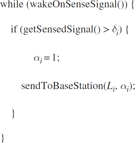
Function wakeOnSenseSignal()puts a sensor in sleep mode until the next sense signal is felt by the sensor node. If the latter happens and the sensed signal strength is greater than δ i (the threshold), it will assign 1 to α i and send its identifier (location Li) and its sense bit (α i ) to the base station. The base station counts these bits (α i ) and considers the count as the weight of location L i ; in other words, α i represents how many times the sensor has sensed an object. Since the sense signals are continuous in time, we will refine our algorithm so that it does not send too many bits to the base station.
On the other hand, sending a bit of data plus the sensor's location to the base station
each time a sensor senses a signal causes too much communication, and the establishment of each
communication interaction is costly in terms of both time and power. Therefore, we can count these
bits at sensor node sides instead of counting them at the base station and then send the aggregated
result to the base station. If we consider α
i
as
an integer variable, we can improve our algorithm as follows: Sensor Node i (improved)
The improved algorithm uses a sleep function to change continuous time to discrete time, where the unit of discrete time is ΔT. We also added T i as a time counter. Each time a sensor senses a new signal, a time counter, Ti, is reset to zero. And each time there is no signal, ΔT is added to the time counter. If there is no signal in a timeout period, it means the object is out of range. Then sensor node i sends L i (its location) and α i (its number of sensed signals) to the base station. Obviously, this improvement greatly reduces the number of communication interactions and saves more energy in the nodes.
α i is used as the weight of L i at the base station to draw the NURBS curve (i.e., the estimation of the path that we want to explore) in our second approach. The use of integer α i , instead of binary α i , shifts the burden of counting operations from the base station to the sensor nodes. This data aggregation reduces the number of communication interactions in the network in exchange for only a slight increase in the computational volume in the sensor nodes. Algorithm 2 sends one data signal per timeout. It waits until the object gets out of its range and then sends its data to the base station once, while Algorithm 1 sends its data continuously as long as it is in the range of the object. So Algorithm 2 is much lighter than Algorithm 1 in terms of communication costs. The simulation results in Section 6 show this fact.
When we draw the b-spline at the base station (in our first step), we do not need the weight for
the location of the sensor that had sensed the object. Every sensor can simply send its location
L
i
to the base station to inform it that sensor
i has sensed the object. We consider this feature in the algorithm to form a
minimal algorithm. Therefore, we developed Algorithm 3: Sensor Node i (minimal)
Algorithm 3 replaces integer α i with binary α i . This causes a reduction in the volume of each network transfer. The number of communication interactions remains the same in both Algorithm 2 and Algorithm 3.
The parameters Timeout i and δ i could be used to tune the sensors; i.e., each sensor node can be configured through a monitoring algorithm to reduce its false alarm rate using Timeout i and δ i parameters.
In Algorithm 2 and Algorithm 3, α i is reset to zero after the ith sensor sends its data to the base station. This enables us to track complex paths that have loops. Resetting α i forces a sensor to consider a new position for a moving object in the final path each time the object repeatedly passes over previously visited positions rather than growing the weight of old positions of the moving object.
If the above algorithm is run on each node, the next step is to find the traversed path of the object, which is achieved by drawing the path's curve. The next section explains how to draw the curve using sensory data (L i and α i ).
Path detection using location data and weights corresponds to the problem of drawing a curve using control points. These curves can be drawn by spline curves. The algorithm for generating a spline curve can calculate a curve in a simple way online that includes control points. Unfortunately, traditional spline curves do not consider the weight of control points and just pass through each point. More complicated algorithms exist for drawing curves using weighted control points. These curves are called NURBS. NURBS calculate the curve by considering the effect of all weighted control points at each point of the curve. A NURBS algorithm is heavy and offline. We use both approaches (b-spline and NURBS) to create the curve of a detected path as described in the next two subsections.
Generating a Path Curve with B-Spline
The mathematical definition of spline is beyond the scope of this article. Readers who are interested in details about spline curves can refer to [14]. Here we present our algorithm for generating a spline. We use a cubic b-spline to create our curve.
The letter b in b-spline stands for the word basic. Each b-spline uses basic
functions to build a point on the final curve. These basic functions determine the influence of each
control point on the final curve. Algorithm
4 shows the b function for the cubic b-spline [15]. Basic B-Spline Function
When creating a b-spline curve, we use a growing factor t (time, in our case).
As t grows, we create another point of the b-spline curve by calculating the basic
functions of four recent control points. The next algorithm calculates the b-spline curve using
function b. B-Spline Curve Function
getXPoint(i) and getYPoint(i) return x and y coordinates of control point i (the location of a sensor). STEPS is used to divide time into fine grain slots. Note that the algorithm uses the last four control points to build the curve as time advances.
Each control point in Algorithm 5 is one of the sensor's locations received by the base station. After choosing the last four control points (outer loop), in each STEP (middle loop), Algorithm 5 calculates a new point in the b-spline curve. To do so, it calculates four b functions (Algorithm 4) for each degree of the polynomial curve, while also calculating the influence of every control point selected by the outer loop on the current point of the b-spline (inner loop).
The time and energy orders of Algorithm 4 and Algorithm 5 are not of concern because these algorithms run at the base station. The order of these algorithms are linear and do not cause any significant problems when the number of sensed data increases.
The main advantage of the b-spline algorithm presented here is that it can be adapted to work with Algorithm 3 (the minimal algorithm described in Section 3), thus reducing the communication load of the network. This means each sensor can only send its location to the base station when it senses an object. The base station then uses Algorithm 4 and Algorithm 5 to produce the path curve.
Another benefit of the b-spline algorithm is its ability to work online. It does not need every control point (received sensor locations) to build the path. As soon as four sensors in the field have sensed an object and have sent their location data to the base station, the base station can start drawing the curve. It can then further complete the curve each time it receives a new sensor's location data.
The main drawback of using a b-spline curve is that each sensor's data highly affects the resulting curve. In other words, the influence of a sensor's data that is located far from the actual path is equal to the influence of a sensor's data that is located near the path. This can lead to reduced precision. In addition, it makes this approach weak against false alarms that can temporarily divert the curve towards false alarm locations.
NURBS is a type of b-spline curve that uses basic functions to determine the influence of each
control point on the curve. Each control point (location of a sensor received by the base station)
influences the curve differently as t (time) advances, so it is called non-uniform
(see knots vector in [14]). In addition, control points in NURBS are weighted so that heavier points have more
influence on the final curve than lighter control points. Another important parameter in NURBS is
k, or the order of NURBS, which determines how much each control point affects each
point in the final curve as t advances. Each control point has k
basic functions. As k grows, more points on the final curve are affected by each
control point. The basic function for control point i and a given
k (order) is defined as follows:
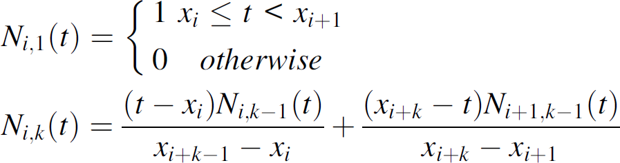
The NURBS curve does not include control points; it just calculates the final curve that passes between them. Each control point inclines the final curve based on its weight and knot vector, resulting in a smooth and precise curve. Larger k values cause each point of the final curve to be affected by more control points. As k grows, the penalty for computation grows as well. However, since computation is performed at the base station, it does not affect the sensors' workloads.
The major benefit of using NURBS is its precision. Since it uses weighted locations to draw the path's curve, it is resistant to false alarms. Because false alarms have low weights, they have little effect on the curve.
The drawback of this approach is that all control points need to be accounted for before calculating the path. It cannot draw the path's curve online because each sensor that has sensed an object must send its location and the location's weight to the base station. In turn, the base station must receive all of this location information before calculating the path, which makes this step offline. Therefore, the NURBS algorithm should only be used to calculate the traversed path after an object passes by all of the nodes.
In the next section, we evaluate our proposed approaches via simulation.
Evaluation
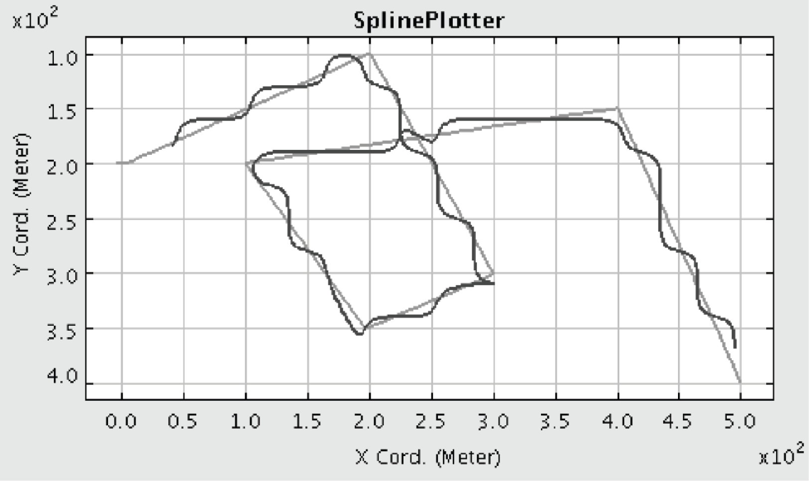
We simulated both proposed approaches with a Visualsense (Ptolemy II) simulator [16]. We developed acoustic sensors using Algorithm 2 and Algorithm 3 to collect and send sensed data to the base station. For the base station, we extended a b-spline plotter and a NURBS plotter from Ptolemy's Plotter component to plot our collected data. Our SplinePlotter class implemented the b-spline algorithms (Algorithm 4 and Algorithm 5) with the postfire() method, which overloads Ptolemy's Plotter to give us an online behavior. Since the NURBS algorithm is offline, we implemented it in the stop() method, which overloads the default plotter's stop(). So the algorithm ran once just before the simulation finished. For simulating mobile objects, we derived a Mobility component from Ptolemy's TypedAtomicActor, which takes a set of targets and cruises between them. We also developed a GPS component for each sensor.
We made two different models to simulate each approach. In the first model, we used 150 sensors evenly deployed in an 850 meter by 700 meter field. The mobile object was an audio source with a 50 meter range that passed through this sensor field. In the second model, we increased the number of sensors to 513. The field was the same as in the first model, but the range of the mobile object was reduced to 20 meters.
To calculate the accuracy of the curves, we assumed a neighboring radius about five meters around the original path. If the detected curve stayed within this neighboring area, we considered it accurate. To determine if this was the case, we calculated the local slope (local derivation) at each point of the original curve. Then we intersected a perpendicular line at that point with the detected curve to find the distance between two curves. If the resulting distance was less than five meters, then we considered the detected curve to be accurate at that point.
We executed our simulations on two different platforms. Our Intel-based PC was a “Lenovo 3000 N100” with 1.83 GHz Core Duo, 1 GB of installed RAM, and a Windows XP operating system. It took about two hours to complete the NURBS calculation with high orders (k = 12) for each complex path. Using a “Sun Ultra 20” workstation with an AMD Opteron Dual Core 2.8 GHz and a Solaris 10 operating system, the computation time was reduced to 35 min for each complex path, thanks to the integrity of Java and Solaris.
We ran each model 100 times to get our results. Our analysis of each simulation result is presented separately below.
Number of Sensors and Object Range
Two parameters that affected the simulation results were the number of sensors in the field and the area of each object's influence.
When the number of sensors was increased, we got better results using NURBS. This is because the number of control points around the actual path increased, leading to better approximation. Figures 1 and 2 show this fact; in both figures, the lighter curve is the actual path, and the darker curve is the detected path. Figure 1 shows the results of running the first simulation model using NURBS with order 6 (k = 6). Figure 2 shows the results of running the second simulation model using NURBS using the same order as in Fig. 1 (k = 6). The comparative results show nearly a 75 percent improvement in the second model in which a larger number of sensor nodes was used. In addition, the range of the mobile object is detrimental. More sensors become involved in wider ranges. This results in more accurate weights and a better approximation of the actual path when NURBS is used.

Path detection using NURBS in the first model (k = 6).

Path detection using NURBS in the second model (k = 6).
Because the b-spline is not weighted and considers equal effects for all sensors, growth in both of the aforementioned parameters resulted in a more spiral curve. Simulation results showed that the best situation for a b-spline occurs with a higher number of sensors and a reduced range of object influence. Figures 3 and 4 show this fact. Figure 3 shows the simulation results of our b-spline approach using the first simulation model. Figure 4 shows the use of our b-spline approach in the second simulation model. In both simulation models, an increase in the number of sensors and a decrease in the range of the object's influence improved our estimation. The simulation results show a more than 50% improvement using the second model as compared to the first model when we drew b-spline curves.

Path detection using b-spline in the first model.

Path detection using b-spline in the second model.
This behavior was expected because only sensors in the actual path were triggered. In addition, a higher number of sensors created more control points in the actual path, leading to a more accurate curve. Based on this behavior, we claim that our b-spline approach is quite appropriate for smart dust sensor technology.
As described before, a higher NURBS order resulted in a more accurate path detection. When we used higher orders for NURBS, we increased the effect of each control point on the final curve. Simulation results confirmed this fact. Figure 5 shows the path curve when we used NURBS with order 12 (k = 12) in the first simulation model. Comparing the results shown in Figs. 1 and 5, we got approximately 60% improvement. Figure 6 shows the resulting path curve using NURBS with order 12 in the second simulation model. This simulation also showed significant improvements again.

Path detection using NURBS in the first model (k = 12).

Path detection using NURBS in the second model (k = 12).
Although higher-order NURBS resulted in a more precise detected path, its computational overhead was so high for an ordinary Intel-based PC (Intel Core Duo 1.83 GHz) that we were forced to switch to high-end Sun workstations (AMD Opteron 2.8 GHz) for our simulations, particularly for getting the results shown in Figs. 5 and 6.
We should point out that this computational overhead does not affect sensor nodes or network lifetime. This is because all computational loads are at the base station; we assume no limitations for necessary resources at the base station.
It is obvious from the figures we presented before that the NURBS approach is more accurate in comparison with the b-spline method, which was expected from our discussions about why NURBS would be more accurate. Our simulation results convey this fact. The comparison of the results shown in Figs. 3 and 5 indicate that the use of the NURBS curve instead of the b-spline curve improves the resulting curve more than 90% using the same model of simulation. Figure 6 (NURBS with order 12) also shows about a 90% improvement compared to the results shown in Fig. 4 (b-spline). The NURBS curve used in Fig. 6 is 95% accurate and is very close to the actual object path. The benefit of using the b-spline approach is its ability to draw the path curve online.
Power Consumption
Since our approach is minimal, in the case of using b-spline, power consumption at each sensor was limited to the power required to send its location to the base station. Each sensor consumed power for just one communication interaction per new simple path (a path without a loop).
The use of Algorithm 2 for creating NURBS entails additional power consumption for sending another integer value besides the node location; this integer (α i ) is the weight of the sensor's location (i.e., how many times the sensor has sensed an object). The computational power consumption in the sensor nodes is the power consumed in Algorithm 2 or Algorithm 3, which is negligible and limited to counting a timer.
To simulate power consumption, we added a battery module to each sensor in Visualsense with an initial power equal to 360 Joules (10% of an AAA NiMH battery capacity). This module consumed energy as the sensor communicates to the base station. We omitted the energy consumed by the sensors for computation, since this energy is incomparably lower than the energy consumed through communication. Communication energy consumption differs for sending and receiving [17]. For receiving data, we simply needed to know how many bits were received in each transfer. We then calculated the receiving energy consumption for l bits as E Rx (l) = E elec × l, where E elec is the radio activation coefficient and is equal to 50 nJ/bit. For sending data, we had to consider the distance to the base station as well. The sending energy consumption for l bits is E Tx (l) = E elec × l + ∊ amp × l × d2 such that ∊ amp is the radio coverage coefficient and is equal to 100 pJ/(bit ∗m2) and d is the distance between the sensor and the base station. For detecting energy consumption in our simulation, each sensor reported its current power to the base station every minute, and the base station added up this information to calculate the network's remaining power.
Energy consumption depends on the speed of the mobile object, ΔT, the path itself, the location of the base station, and so on. But in a constant situation, we could compare the energy consumption of the different algorithms. On average, the sensors in our approaches consumed below 0.0005% of the network's energy for each mobile object using Algorithm 2 or Algorithm 3, while they consumed nearly 0.005% of the network's energy using Algorithm 1.
Thus, the simulation results show that power consumption in both approaches is ultimately low.
Complex Paths
Our approaches are capable of determining complex paths including loops and extreme curves. Figures 7 to 10 show the effectiveness of both approaches in following more complex paths.

Complex path using b-spline in the first model.
Complex path using b-spline in the second model.

Path detection using NURBS in the first model (k = 6).

Path detection using NURBS in the second model (k = 12).
Figures 7 and 8 illustrate that the b-spline approach can determine complex paths just as effectively as simple ones. Also, we can see that increasing the number of sensors in the second model leads to a better path estimation. The accuracy of the b-spline approach in complex paths was generally between 50 and 8%. The NURBS approach can also determine complex paths; Figs. 9 and 10 show this fact.
The accuracy of the NURBS approach depends on the same parameters described before. Again, the use of the second model improved our accuracy in the NURBS approach. The average resulting accuracy using NURBS for complex paths ranged from 60 to 90% on the different paths.
Due to problems in implementation, our simulations could not detect multiple paths simultaneously. They could only detect one path at a given time even though more than one mobile object could traverse that path. Using a neighboring detection algorithm and some clustering [7] could enhance multiple path detection. This issue is left for future research.
This article presented two approaches for finding available paths in unknown areas using a binary sensor network. In the first approach, each sensor sends its own location to the base station when it senses an object of interest, and the base station uses b-spline curves to build the object's path online. Since each sensor sends its location data just once per new path, it is a minimal approach. The path is (re)built by the base station every time it receives a new location. The second approach uses NURBS instead of b-spline to detect an unknown existing path. Since NURBS needs weighted locations, each sensor sends the number of times it has sensed the object based on the object's weight and its own location. The second approach is an offline approach.
Both approaches were simulated with a Visualsense (Ptolemy II) simulator to evaluate their accuracy in detecting paths. The simulation results showed that the path detected by the second approach (NURBS) was 90% more accurate than the one detected by the first approach (b-spline) using the same model of simulation. The accuracy of the NURBS approach was further shown to be nearly 95% accurate in the simulated results, which was very close to real path. Our second approach was also robust on false alarms. We intend to extend the NURBS approach to detect multiple paths simultaneously and online.