Sage Journals: Discover world-class research

Abstract

Some object tracking applications can tolerate delays in data collection and processing. Taking advantage of the delay tolerance, we propose an efficient and accurate algorithm for in-network data compression, called delay-tolerant trajectory compression (DTTC). In DTTC, a cluster-based infrastructure is built within the network. Each cluster head compresses an object's movement trajectory detected within its cluster by a compression function. Rather than transmitting all sensor readings to the sink node, the cluster head communicates only the compression parameters, which not only provide the sink node expressive yet traceable models about the object movements, but also significantly reduce the total amount of data communication required for tracking operations. DTTC supports a broad class of movement trajectories using two proposed techniques, DC-compression and SW-compression, and an efficient trajectory segmentation scheme, which are designed for improving the trajectory compression accuracy at less computation cost. Moreover, we analyze the underlying cluster-based infrastructure and mathematically derive the optimum cluster size, aiming at minimizing the total communication cost of the DTTC algorithm. An extensive simulation has been conducted to compare DTTC with competing prediction-based tracking technique, DPR [28]. Simulation results show that DTTC exhibits superior performance in terms of accuracy, communication cost and computation cost and soundly outperforms DPR with all types of movement trajectories.

Keywords

Compression Segmentation Object Tracking Wireless Sensor Networks

1. Introduction

Object tracking is a killer application of wireless sensor networks. In this application, the sensor nodes collectively monitor and track the movements of moving objects. As other types of sensor network applications, object tracking in sensor networks is constrained by limited on-board, non-refreshable battery power, computation capability, and storage. This has spurred a need for designing techniques tailored specifically toward object tracking sensor network environments to allow optimized tradeoff between the energy consumption, network performance, and operation fidelity.

A wide range of object tracking applications can be categorized into real-time tracking and delay-tolerant tracking. In real-time object tracking, since a sink node watches the movements of a moving object closely, the sensor readings are collected in real time. For instance, a battle field surveillance application requires real-time tracking of enemy soldiers to facilitate prompt decision making. Other real-time tracking applications include highway navigation, emergency warning, and disaster rescue [3, 13]. On the contrary, in delay-tolerant object tracking, a sink node can tolerate a delay in collecting sensor readings. For example, in wildlife habitat monitoring, scientists only need to know the approximate movement trajectory of a group of zebras, instead of their real-time movements [21, 30].

The existing tracking techniques in sensor networks are usually designed to meet real-time requirements. In order to avoid continuous updates about locations of tracked objects from sensor nodes to the sink node, many existing tracking techniques predict the future locations of a moving object based on its movement history [1, 9, 14, 26, 28, 29]. The basic idea is described as follows: when the prediction made by a sink node is correct, sensor nodes do not report their readings to the sink node. Otherwise, sensor nodes correct the sink node by sending their readings. However, in practice, the movement trajectory of moving objects is complex. Individual objects may exhibit completely different movement patterns, which poses significant challenges for a prediction-based tracking technique to accurately predict the object movements. Moreover, some prediction-based techniques derive movement probability models from the movement history of a group of objects that share the similar movement pattern. The future movements of a moving object are predicted based upon the corresponding movement prediction models. However, these techniques make a strong assumption that there are a small number of movement states (e.g., moving speed and direction) that a moving object can follow, such that prediction models can be stored locally at the sensor nodes and the probability for an object taking a future movement state can be calculated efficiently.

In addition to the above deficiencies, the prediction-based tracking technique is not the best choice for delay-tolerant object tracking, which, by releasing the timeliness requirement, provides significant opportunities for optimizing other performance metrics in tracking operations, e.g., communication cost. In this paper, we investigate a novel technique, called delay-tolerant trajectory compression (DTTC), for delay-tolerant object tracking sensor networks. DTTC is able to present a sink node accurate movement trajectory of a moving object at significantly decreasing communication cost. Specifically, in DTTC, a cluster infrastructure is organized inside the network. Each sensor node reports its readings to the cluster head for further signal processing and data aggregation. This infrastructure is widely used in wireless sensor networks for improving energy efficiency in various operations, such as data fusion and in-network processing [7, 11]. Instead of sending the object's locations at consecutive time instants, the cluster head aggregates and compresses those data by a compression function and only sends a set of compression parameters that model the movement trajectory of the tracked object to the sink node. To compress a complex movement trajectory precisely and efficiently, DTTC employs a trajectory segmentation technique, which divides the whole trajectory into segments, and applies a relatively simple compression function to each segment. However, obtaining segments with the right length is not a trivial task. One straightforward solution is to divide the trajectory evenly into segments with the same length, without considering the trajectory shape. This approach could lead to unnecessary segmentation for the trajectory which is smooth enough to be compressed by one function, and there is insufficient segmentation when more segments are needed. As a result, both compression error and computation overhead increase. In this paper, we study an intelligent trajectory compression method, which, by taking into consideration the pattern in movement trajectory, forms segments with the right length in one scan of given data. Upon obtaining segments, two compression techniques, namely, DC-compression and SW-compression, are studied for different object movement patterns. In addition to the trajectory compression technique, we study the impact of the underlying cluster infrastructure on DTTC's communication cost, by considering tracking factors and parameters (including reporting duration, object's moving speed, network scale, and size of transmitted packets). The optimum cluster size is mathematically derived aiming at minimizing communication cost. Our contribution can be summarized as follows:

We propose the DTTC technique for delay-tolerant object tracking in wireless sensor networks. DTTC compresses a sequence of location points that depict the movement trajectory of a tracked object into a set of compression parameters. DTTC significantly decreases the total amount of data communication in the tracking operation.

We carefully craft a trajectory segmentation scheme, which segments a trajectory with one scan of the data. The scheme empowers DTTC the ability of precisely and efficiently compressing complex trajectory that has frequent changes in movement states (e.g., moving directions).

Two trajectory compression techniques, DC-compression and SW-compression, are proposed to reduce the computation overhead for different movement patterns.

We analyze the impact of cluster infrastructure on the communication cost of DTTC and mathematically derive an optimum number of clusters, aiming at minimizing the total energy consumption. The analysis provides important insights on configuring the cluster infrastructure and optimizing the performance of DTTC.

We provide an extensive experimental study of a proposed DTTC technique with various movement trajectories (i.e., both linear and non-linear movements) and make comparisons against a prediction-based tracking technique. DTTC demonstrates superior performance in accuracy, communication cost, and computation cost.

The rest of the paper is organized as follows. Section 2 examines the related work. In Section 3, we state the tackled problem, and present the design of DTTC. Section 4 analyzes the appropriate cluster size for use in DTTC and Section 5 reports experimental results. Finally, Section 6 presents concluding remarks.

2. Related Work

Due to the extremely frugal power budget for sensor nodes, energy usage is one of the most critical factors that determine sensor network applicability in reality. Network communications, especially long-distance communications, are identified as the power bottleneck in sensor network systems, thus becoming the target area of various optimizations [12, 22]. With the same design goal as much existing work, we examine some energy-saving techniques proposed for communication reductions for sensor networks¹

2.1. Suppression and Prediction

Two primary strategies used for reducing sensor network communication are suppression and prediction. These two techniques both achieve energy efficiency by keeping sensor nodes from transmitting data. Suppression is based on local collaborative information processing; while prediction, by involving higher-level applications, is categorized as a wide-area collaborative information processing technique [23].

Suppression. Suppression is effective in many sensor network applications, such as habitat monitoring, where conditions change slowly or rarely. Suppression techniques can be categorized into

temporal suppression: each node reports its readings only if the reading changes noticeably since its last transmission. However, when all nodes change, limited energy savings can be achieved.

spatial suppression: sensor nodes suppress transmissions when their readings are close enough to their neighbors.

Some exiting energy-efficient protocols designed for sensor networks, including [19, 24, 25], utilize suppression techniques. However, sensor readings about object movements (e.g., locations of a moving object) do not have strong temporal or spatial correlations.

Prediction. Prediction techniques have been extensively studied, including for object tracking sensor networks [1, 9, 14, 15, 26, 28, 29, 31]. The prediction-based object tracking techniques assume the overall movement states (e.g., direction and speed) of tracked objects usually remain relatively stable for a period of time. The sink node predicts the future movement of a tracked object based on the movement history, and sends its prediction to the corresponding sensor nodes. If the prediction matches the sensor readings, no sensor reports are needed. Otherwise, the sensor nodes correct the sink node by sending their own readings. [26, 29, 28] further improve this technique by a dual prediction scheme, in which the predictions take place at both sensor nodes and the sink node. To predict an object's future movements, sensor nodes pass the object's movement history along its movement trajectory. The sensor nodes send the updates to correct the sink node when the prediction is found to be wrong.

Based on the movement history used for prediction, prediction techniques can be classified into prediction with individual history and prediction with group history. The prediction with individual history (e.g., [9, 26, 28, 29]) predicts the movement of an object from its own history. Considering the randomness in object movements in practice, simple prediction models in the existing work (e.g., CONSTANT, AVG, EXP_AVG) could result in poor prediction performances, which in turn incurs more communication for correcting the sink node. The prediction with group history for a moving object is made based on the movement history of all objects that share the same movement pattern with the tracked object. Group history provides richer information about object movements, thus more advanced techniques can be applied to extract the movement pattern for a group of objects [1, 4, 8, 14, 18].

However, these techniques assume a limited (and small) number of movement states (e.g., moving speed and direction) that an object can have, such that probability for objects taking each state can be calculated and used for future predictions.

2.2. Aggregation

Aggregation techniques are also widely used for reducing network communications [5, 6, 10, 16, 17, 20, 27]. Different from suppression and prediction techniques, aggregation techniques do not restrain sensor nodes from reporting their readings, but try to reduce the total amount of data transmitted.

There are two types of aggregations. The first approach, called the operator-based approach, reduces data communications by performing simple aggregation according to the query operator specified by the application, such as MAX, MIN, AVG, COUNT, and SUM [5, 16, 17, 20, 27]. However operator-based aggregation may lose much of the original structure in the data, providing coarse statistics that smooth over interesting local variations. The aggregation result can only answer one or a few types of queries. Moreover, operator-based approaches are not feasible for object tracking sensor networks, which is interested in obtaining continuous objects' movement states. The second aggregation approach, called the model-based approach, is a more general aggregation technique [10, 20]. Our proposal DTTC falls into this category. The model-based approach focuses on capturing and modeling the correlations existing in a set of sensor readings. Rather than sending all raw sensor readings to the sink node, the network only reports the model parameters, from which the sink node can reconstruct the shape and the structure of the ordinal data. Different from the existing model-based aggregation techniques, DTTC faces different research challenges. First, the movement states of an object may change frequently, such that it is impossible to use one model to capture the entire trajectory. Furthermore, supported by a cluster-based infrastructure, the configuration of the clusters is critical to the performance of DTTC. We address these issues in this paper.

3. Design of Delay-Tolerant Trajectory Compression

We first discuss the basic idea of delay-tolerant trajectory compression (DTTC) in Section 3.1. The detailed trajectory segmentation scheme and compression techniques are discussed in Section 3.2 and Section 3.4, respectively.

3.1. Basic Idea of DTTC

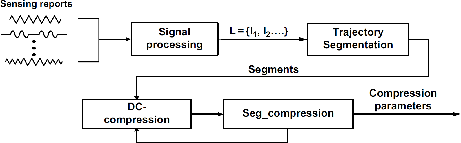
In DTTC, a cluster infrastructure is formed within the network where sensor nodes report their readings to the cluster head for data fusion². Reporting duration, a period of time between two consecutive sensor reports from sensor nodes, is specified by the object tracking applications. To simplify our presentation, we assume that the sensor nodes have synchronized clocks. However, our work can be easily adapted for unsynchronized networks. At time t, a set of sensor nodes that detect the moving object participate in object tracking and report their readings to the cluster head. A report packet from a sensor node is denoted by <t, R, S_id, O_id>, where R represents the sensor readings from node S_id about moving object O_id stamped at time t. As multiple sensor nodes may detect and track the same moving object, the cluster head is likely to receive several sensor reports with the same time stamp. By processing multiple reports with the same t (shown as signal processing in Fig. 1), the cluster head derives the movement state, i.e., geographical location, for object O_id at time t, denoted as <t, x, y, O_id>, where x and y are the geographical coordinates for O_id at t by assuming a two-dimensional space.

Figure 1

DTTC with DC-compression technique.

Instead of reporting to the sink node the movement trajectory of object O_id, represented by a sequence of geographical locations denoted by L = {l₁, l₂, …}, l_i = <t_i, x_i, y_i, O_id> at time t₁, t₂, …, the cluster head performs a trajectory compression upon L , denoted as Trajectory_Compression ( L ). The output of Trajectory_Compression ( L ) is sets of (β, ∊), where β is the compression parameters derived from trajectory compression, and ∊ is the corresponding compression error that should be less than the tolerant compression error bound ξ. After the trajectory compression, the cluster head reports β and other necessary information (will be discussed shortly in Section 3.1) to the sink node.

Trajectory_Compression operations in DTTC focus on compressing movement trajectory L = {l₁, l₂, …} using a compression function, which could be a linear function, quadratic function, and etc. For instance, a quadratic function, ŷ = β₀ + β₁x + β₂x² can depict many kinds of moving pattern via different parameter β₀, β₁ and β₂. This compression function can also capture linearity as a special case (and therefor has higher applicability). However, with a degree of 2, a quadratic compression function can only capture a trajectory with one turning point, and is not applicable for more complicated trajectories (e.g., with more turning points). Furthermore, a compression function with higher degree, in addition to increasing the computation complexity, may still not be applicable to all kinds of movement trajectory. A possible solution to the above problem is that a cluster head caches a set of compression functions that capture various movement patterns. Given a movement trajectory L , the cluster head tries each compression function on L , and selects the function that yields the smallest compression error. The drawbacks of this approach are obvious. First, it requires extra storage space for caching a number of compression functions. Second, with a large number of compression functions cached, the cluster head may still fail to find a matching function for an arbitrary movement trajectory with mixed movement patterns.

DTTC addresses the above problem based on the observation that a trajectory can be segmented. The piece-wise segments can be approximated with a relatively simple compression function (e.g., a quadratic model or even a linear model when the segments are small enough). In the following, we present the compression techniques for a given segment, followed by two alternative compression techniques and a trajectory segmentation scheme. The overview of DTTC with DC-compression technique is shown by Fig.1. DTTC with the SW-compression technique has a similar flow.

3.2. Segment Compression

A segment S is characterized by a set of parameters:

t_s and t_e: the timestamps representing the time when the first and last l in segment S are generated by the sensor nodes, i.e., S(t_s, t_e) = {l_i = <t_i, x_i, y_i, O>|t_s  t_i < t_e}, and thus determining the length of a segment. We denote x(t_s, t_e) = {x_i|x_i ∊ S(t_s, t_e)}, and y(t_s, t_e) = {y_i|y_i ∊ S(t_s, t_e)}.

x_t_s and x_t_e: the x-coordinates of the first l_t_s and of the last l_t_e in segment S. These two values are used by the sink node to reconstruct the movement trajectory of an object.

β and ∊: β represents the compression parameters of segment S, and β = (β₁, β₂, …, β _m ). ∊ is the error introduced by the compression on a segment S. In this paper, we adopt the root mean squared error (RMS), which is widely used as the error metric in regression techniques. Other error metrics can also be used by DTTC with minor changes.

Subroutine Seg_Compression() shown in Algorithm 1 is at the core of DTTC. This function compresses a segment of movement trajectory, i.e., S(t_s, t_e), and computes the regression parameters β, as well as the compression error ∊. The compression function is represented as

y (t_{s}, t_{e}) = \sum_{j = 0}^{m} Φ_{j} (x (t_{s}, t_{e})) β_{j}

where Φ₀, Φ₁, …, Φ_m are functions of x(t_s, t_e). For instance, when Φ₀ = 1, Φ₁ = x(t_s, t_e), …, Φ_m = x(t_s, t_e)^m, y(t_s, t_e) = β₀ + β₁x(t_s, t_e) + … + β_mx(t_s, t_e)^m. By setting reporting duration as one time unit, the compression function can be represented in vector notation,

[\begin{matrix} y {\hat{t}}_{s} \\ y {\hat{t}}_{s} + 1 \\ \cdot \\ \cdot \\ y {\hat{t}}_{2} \end{matrix}] = [\begin{matrix} Φ_{0} (x_{t_{s}}) & Φ_{1} (x_{t_{s}}) & \dots & Φ_{m} (x_{t_{s}}) \\ Φ_{0} (x_{t_{s} + 1}) & Φ_{1} (x_{t_{s} + 1}) & \dots & Φ_{0} (x_{t_{s} + 1}) \\ \cdot \\ \cdot \\ Φ_{0} (x_{t_{e}}) & Φ_{1} (x_{t_{e}}) & \dots & Φ_{m} (x_{t_{e}}) \end{matrix}] [\begin{matrix} β_{0} \\ β_{1} \\ \cdot \\ \cdot \\ β_{m} \end{matrix}]

Algorithm 1

Seg_Compression()

Algorithm 1 can be executed once a segment is identified. A naive way of constructing segments is to divide the movement trajectory L evenly into a number of segments, and strictly applying algorithm 1 on each segment. However, as stated in Section 3.1 our goal is to reduce the total amount of data communications, evenly segmenting a movement trajectory cannot guarantee that DTTC reaches the goal. There are two possible approaches to tackle the above problem:

to minimize the total number of segments, which, however, may generate more parameters for each segment, as a longer segment of movement trajectory is very likely to require a more complicated compression function with more compression parameters;

to minimize the number of parameters (i.e., β) for each segment, which implies using simpler compression functions. In this case, to ensure ∊ < ξ, the total number of segments may increase. As the compression function is usually pre-determined by applications, we study two compression techniques that aim at minimizing the total number of segments to be compressed for a given compression function (e.g., a m-degree of polynomial compression function).

3.3. Compression Techniques

We introduce two compression techniques, namely, Divide-and-Conquer compression (denoted as DC-compression) and Stepwise compression (denoted as SW-compression), both of which aim at minimizing the total number of segments and reducing the total amount of data communications, with a given compression function. Meanwhile, these two techniques target on different movement patterns that an object may follow. We assume that the movement trajectory of a moving object L is stored in an ascending chronological order at a cluster head.

3.3.1 DC-Compression

The DC-compression is based on the idea of divide-and-conquer. The compression takes place after the cluster head obtains all data that need to be compressed.

Without loss of generality, we assume there are N data entries available at a cluster head when it performs compression, denoted as L = {< t₁, x₁, y₁, O >, < t₂, x₂, y₂, O > …, < t_N, x_N, y_N, O >}, which depict the locations of moving object O at different time stamp reported by different sensor nodes. The DC-compression, shown in Algorithm 2, works recursively. At the beginning, it takes the entire trajectory inside the cluster, i.e., L , as one segment. In each iteration, the segment with the largest compression error is selected and divided into two segments at timestamp t_div. A critical research issue in DC-Compression is to select t_div for the segment that has the largest compression error in an iteration. One approach is to divide a segment into halves, such that t_div = [(t_emax — t_smax)/2], where t_emax and t_smax are t_s and t_e for the segment with the largest compression error. However, this solution may cause too many segments and increase the compression errors, as the selection of t_div does not consider the pattern in the movement trajectory. The selection of t_div will be discussed in detail shortly in Section 3.4. The above process repeats until the maximum number of segments is exhausted or the compression errors of all segments are less than the error bound ξ. The compression parameters for a segment can be reported to the sink node once its compression error ∊ < ξ.

Algorithm 2

DC_Compression()

3.3.2 SW-Compression

The DC-compression aims at maximizing the size of each segment and reducing the total number of segments. However, DC-compression incurs a high computation cost when the movement trajectory within a cluster in nature has to be divided into multiple segments for compression, since its compression starts from the entire trajectory within a cluster.

In this section, we introduce another compression technique, called Stepwise compression, or SW-compression in brief. Similar to DC-compression, the movement trajectory L = {l₁, l₂, …, l_N} of an object is segmented. The algorithm Seg_Compression is applied to each segment. Taking a different approach, the SW-compression first divides the trajectory into segments. The compression starts from a single segment, instead of the entire trajectory within the cluster as the DC-compression does. SW-compression tries to compress as many segments in one compression function as possible. More specifically, SW-compression involves

selecting an initial segment and compressing it;

adding the next new segment to the current segment that has been compressed, compressing the combined segment, and obtaining new compression parameters and compression errors;

terminating step 2 when either no new segment is left or the obtained compression error exceeds ξ. The above process is repeated until the maximum number of segments is exhausted or there is no segment left. Algorithm 3 depicts the SW-compression technique.

Algorithm 3

SW_Compression()

Segmentation is critical for SW-compression. Similar to the discussion about DC-compression, a straightforward approach for constructing segments in SW-compression is to divide L into a number of segments with the same size. However, the size of a segment is hard to determine. If the size of a segment is too small, the computation cost would be high, as the compression is conducted whenever a new segment is added. This computation overhead seems unnecessary, when the movement trajectory of an object is smooth, which likely requires less number of segments. On the other hand, when the size of a segment is large and the movement trajectory of an object is complex (e.g., with many turning points), the compression error would increase. In this case, a large segment has to be further divided into small pieces. Thus, for both DC-compression and SW-compression, trajectory segmentation has to take into consideration the movement trajectory of the moving objects, for reducing both computation cost and compression error.

3.4. Trajectory Segmentation

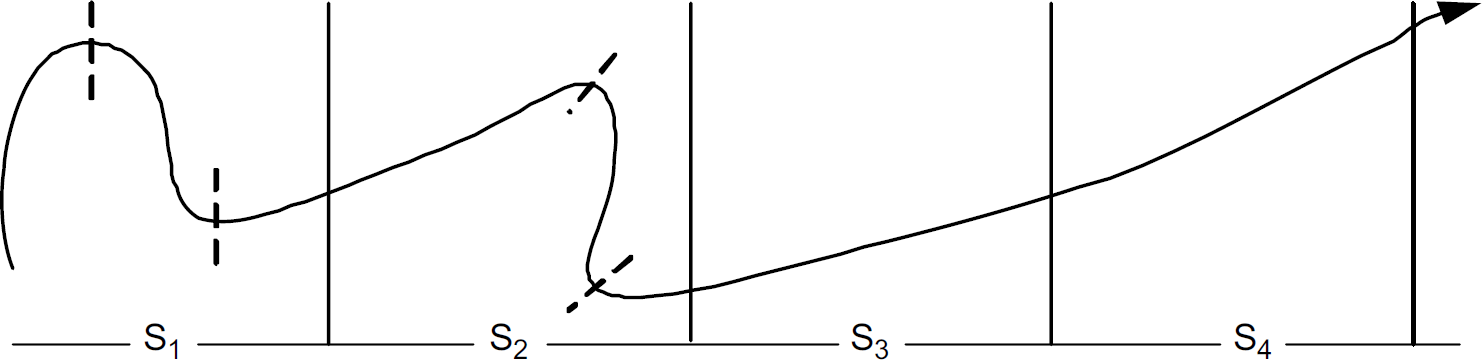
A simple segmentation approach is evenly dividing the trajectory into segments as shown in Fig. 2 . Apparently this approach has deficiencies. In Fig. 2, the trajectory shown by the solid arrow is evenly divided into four segments i.e., S₁, S₂, S₃, S₄, with the same length. However, we observe that S₁ and S₂ contain one or more turning points (i.e., the intersection between the trajectory and the dashed line). Thus, it is difficult to compress them by one simple function without hurting the compression accuracy. On the contrary, S₃ and S₄, which are smooth and have a similar pattern, can be combined into one segment for compression. In this work, we consider a different segmentation approach that takes into consideration the trajectory pattern and aims at minimizing both communication and computation cost.

Figure 2

Trajectory segmentation.

A good trajectory segmentation scheme should satisfy the following two requirements:

the formed segments have the right length. More specifically, the segment should be short enough, such that it can be compressed by a compression function with ∊  ξ. Meanwhile, in order to reduce both communication and computation overhead, a segment should not be too short;

trajectory segmentation should not incur excessive computation overhead. In the following, we study a trajectory segmentation scheme that divides a given trajectory into segments in one scan of given data. The focus is on forming segments with the right length, while being resilient to complex movements.

Studying a movement trajectory, the turning points on both y-axis and x-axis are the main reason that a compression function fails to compress the trajectory accurately. Turning points, represented as the local maxima and local minima (together refereed as local extremum), are mainly caused by the dramatic changes in moving direction. Therefore, by examining the location points l₁, l₂,…,l_N along the movement trajectory of a moving object, the cluster head can perform segmentation along t when local extremum on either x- or y-axis are identified. In the following, we present how a cluster head segments the movement trajectory based on local extremum by taking the local extremum on x-axis as example. Y-axis can be processed in the same manner.

The cluster head continuously obtains a sequence of location points along the object's movement trajectory l₁, l₂, l₃,…. At the beginning, the cluster head initializes l_max = l_min = l₁, where l_max = < t_max, x_max, y_max, O> records the local maxima at x-axis and l_min = <t_min, x_min, y_min, O> records the local minima at x-axis. For a new arrival of l_i, if x_i > x_max, l_max = l_i; otherwise if l_i < x_min, l_min = 1_i. With a small enough reporting duration, it is unlikely that both l_max and l_min are to be set as l_i. We denote $\vec{d} (t_{i})$ as a general moving direction of the moving object between t_i and t_i+1. $\vec{d} (t_{i}) = 1$ , when x_i+1 > x_i, otherwise $\vec{d} (t_{i}) = - 1$ . In reality, the object movement trajectory would not be perfectly smooth, such that a large amount of local extremum could exist. In this case, a cluster head, when performing segmentation, needs to ignore the bumps that are the local extremum but only slightly deviates from the overall movement trajectory. If $\vec{d} (t_{i}) \vec{d} (t_{i + 1}) > 0$ , no bump or segment needs to be identified and the cluster head continues to examine succeeding location points. Otherwise, if $\vec{d} (t_{i}) \vec{d} (t_{i + 1}) < 0$ , the cluster head places a mark on l_i+1 by l_bump = l_i+1 and examines the location points l_i+2, l_i+3,… to decide whether it is just a bump, or a new segment should be formed. There are two possible cases:

$\vec{d} (t_{i}) = 1$ : Let j = 2, 3, … If $\vec{d} (t_{i}) \vec{d} (t_{i + j}) > 0$ , the cluster head considers location points l_i+2, l_i+3, …, l_i+j–1 as small deviations from the object's movement trajectory, ignores them in segmentation, and clear l_bump. Otherwise, if $\vec{d} (t_{i}) \vec{d} (t_{i + j}) < 0$ , the cluster head calculates the geographical distance between l_bump and l_i+j+1, i.e., B = ((x_bump – x_i+j+1)² + (y_bump – y_i+j+1)²)^1/2. If B  B_max, the cluster head forms a segment between t_min and t_max, clears the l_bump, and resets l_max = l_i+1 and l_min = l_i+j+1 for the next segment. If B < B_max, j increases by 1.

$\vec{d} (t_{i}) = - 1$ : This is similar to the previous case, except that the new segment is formed by setting l_min = l_i+1 and l_max = l_i+j+1

The above trajectory segmentation only requires one scan of all data to be compressed, to find out the local extremum for constructing segments. Each formed segment tolerates small deviations in object movements.

4. Performance Analysis

In this section, we analyze the performance of DTTC, paying special attention to the cluster size of the underlying cluster infrastructure. We argue that cluster size is an important parameter affecting the energy efficiency of DTTC, which is a critical performance metric for sensor network based applications.

The total communication cost incurred under normal operations of DTTC consists of

intra-cluster cost: It is the communication cost within a cluster. It is incurred in the process of collecting sensor reading to the cluster head for the later trajectory compression.

cluster-sink cost: It is caused by the communication of compression parameters from cluster heads to the sink node, which using these packets, recover the object moving trajectory.

Given the above two communication costs, larger clusters increase the intra-cluster cost, which likely dwarfs the savings in cluster-sink communication. Meanwhile, with smaller clusters, more communication between cluster-sink is incurred, which, considering a large-scale network, could result in high communication cost. Therefore, the cluster size is a key factor in optimizing the performance of DTTC. Our analysis is based on the following assumptions:

The object maintains its velocity for a period of time before any change

For simplicity, we assume the object moves linearly

The number of hops between two nodes is proportional to the geographical distance between them. Specifically, we define the number of routing hops between two nodes as the ratio of the geographical distance between these two nodes to the communication range R.

Figure 3(a) shows an example of data collection within a cluster, where the grey dashed arrow represents the moving trajectory of an object, and t₀ to t₄ denote five time stamps when the sensor nodes report their readings about the object trajectory to the cluster heads. The geographical distance between adjacent time stamps is a constant, denoted as u, as we assume the object moves linearly with relatively constant speed. u is calculated as product of |t_i+1 – t_i| and object's moving speed, where |t_i+1 – t_i| is the reporting duration. In this example, we assume a cluster is a circle centered at the cluster head with C as radius. All sensor nodes falling into this region report their readings to the cluster head upon detecting the object at the required time stamp. We draw an x-axis and a y-axis, which intersect at the point where the object enters the cluster, shown by grey solid arrows in Fig.3(a).

Figure 3

Performance analysis.

We first consider intra-cluster cost. As shown in Fig.3(b), the coordinates of the point where the object enters the cluster and of the cluster head are (0,0) and (C, 0), respectively. For simplicity, we assume a report is generated when the object enters the cluster (i.e., at time stamp t₀). Giving a time stamp t_i, which is i∗ u away from t₀, the energy consumed to report to the cluster head is

e^{*} B_{d a t a} * \frac{\sqrt{(i^{*} u)^{2} + C^{2} - 2 C^{*} i^{*} u c o s θ}}{R}

where e represents the energy consumed by transmitting a unit of data for one hop, B_data denotes the size of a sensor reading packet generated by sensor node, and θ is the angle formed by the object's trajectory and x-axis in Fig. 3 (b). The total number of packets generated for reporting the object's locations within the cluster is $\frac{2 C c o s θ}{u}$ . Therefore, for a given trajectory with angle θ, the intra-cluster cost is

\sum_{i = 0}^{\frac{2 C c o s θ}{u}} e^{*} B_{d a t a} * \frac{\sqrt{(i^{*} u)^{2} + C^{2} - 2 C^{*} i^{*} u c o s θ}}{R}

Giving the cluster radius C, the average intra-cluster cost, denoted by E_data(C) is

E_{d a t a} (C) = (\int_{- \frac{π}{2} + ϑ}^{\frac{π}{2} - ϑ} \sum_{i = 0}^{\frac{2 C c o s θ}{u}} e^{*} B_{d a t a} * \frac{\sqrt{(i^{*} u)^{2} + C^{2} - 2 C^{*} i^{*} u c o s θ}}{R} d θ) / π

where ϑ represents a very small angle such that $θ \in (\frac{π}{2}, \frac{π}{2})$ .

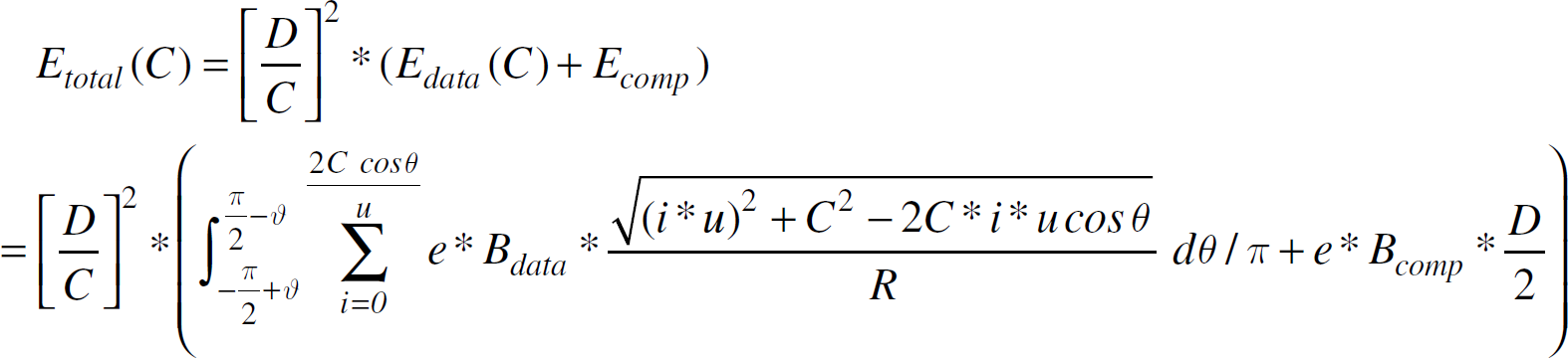
Now, we consider the average cluster-sink cost, giving cluster radius C. Assuming a disk-shaped network region with radius D, the average distance between a cluster head and the sink node, which locates at the center of the network, is $\frac{D}{2}$ , and the cost of transmitting one packet of compressed trajectory from a cluster head to a sink node, denoted by E_comp is $E_{c o m p} = e^{*} B_{c o m p} * \frac{D}{2}$ , where B_comp is the size of a compression packet generated by the cluster head. We assume that all clusters will be traversed, giving a long enough period of time. Therefore with cluster radius C, the average total cost for the sink node obtaining the object's moving trajectory, denoted by E_total(C) is

\begin{aligned} E_{t o t a l} (C) = {[\frac{D}{C}]}^{2} * (E_{d a t a} (C) + E_{c o m p}) \\ = & {[\frac{D}{C}]}^{2} * (\int_{- \frac{π}{2} + ϑ}^{\frac{π}{2} - ϑ} \sum_{i = 0}^{\frac{2 C c o s θ}{u}} e^{*} B_{d a t a} * \frac{\sqrt{(i^{*} u)^{2} + C^{2} - 2 C^{*} i^{*} u c o s θ}}{R} d θ / π + e^{*} B_{c o m p} * \frac{D}{2}) \end{aligned}

To minimize E_total(C),

C^{*} = a r g_{C \in (1, M)} m i n {E_{t o t a l} (C)}

Figure 4 illustrates the optimal number of clusters (i.e., ${[\frac{D}{C^{*}}]}^{2}$ ), under various distances an object traverses within a reporting duration (u), network radius (D), and the ratio of the compression packet size to the data packet size (B_comp/B_data). Generally, we observe that the optimal number of clusters is large when B_comp/B_data is small, and it decreases, as B_comp/B_data becomes larger. This can be explained as follows. When the ratio of B_comp/B_data is small, the cluster-sink cost is small. In this case, it is beneficial to form more clusters with smaller size to reduce the intra-cluster cost. When B_comp/B_data increases, the communication cost in transmitting compression packets from cluster heads to the sink node increases, such that it is necessary to reduce the total number of clusters to reduce the cluster-sink cost. When the ratio of B_comp/B_data is fixed, the optimal number of clusters increases as the network expands, which is denoted by the ratio of the network radius over the communication range D/R. Comparing Fig.4(a) with Fig.4(b), the optimal number of clusters decreases when u increases. Because less intra-cluster cost is incurred with increasing u, such that the cluster with a larger size is preferred. The impact of u will be further studied in Section 5.4. Finally, we want to point out that considering the assumption made for the above analysis, the derived optimal number of clusters may not necessarily yield the minimum communication cost in practice. However, the analytical results provide profound insights and important guidance for determining the optimal cluster size and designing the energy-efficient DTTC algorithm. This remark is further verified by our experimental results in Section 5.2.

Figure 4

The optimal number of clusters.

5. Performance Evaluation

In this section, we study the impact of different choices in protocol design (including the number of clusters and error bound ξ) on the performance of DTTC. We also compare the performance of DC-compression and SW-compression techniques and examine DTTC's sensitivity to system and application parameters, such as the moving speed of objects and reporting the duration from sensor nodes.

5.1. Simulation Settings

We implement all schemes under comparison in MATLAB. We assume a sensor network is deployed in a 1000m × 1000m two-dimensional region. Without loss of generality, the network region is divided evenly into a number of clusters, and a cluster head is placed in the middle of each cluster. The transmission range of a sensor node is set to 40m [12], and the node density, i.e., the average number of neighbor nodes in the transmission area of a sensor node, is 20. The number of hops for transmitting a packet is approximated as the ratio of the routing distance to the transmission range of a sensor node (i.e., 40m).

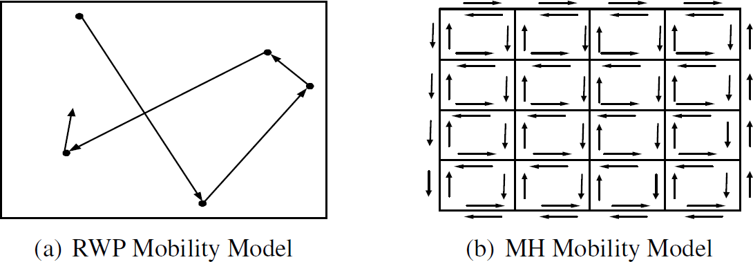
We consider two kinds of trajectories, i.e., linear and nonlinear movement trajectory. With linear movement trajectory, an object moves with a fixed moving direction for a period of time before changing its direction. On the other hand, an object following nonlinear trajectory keeps changing its moving direction. To simulate the linear movement trajectory, we employ the following two mobility models:

Random waypoint mobility model (RWP): RWP model has been widely used for modeling ad hoc movement patterns. RWP (as shown in Fig. 5 (a)) runs as follows: at every instant, an object randomly chooses a destination and moves towards it with a constant velocity.

Manhattan mobility model (MH): MH (as shown in Fig. 5 (b)) emulates the movement pattern of a moving object on streets defined by a map. The map is composed of horizontal and vertical streets. Each street is bidirectional. We adopt MH settings used by [2]: at the intersection of streets, a moving object can turn left, turn right and go straight with a probability of 0.25, 0.25, and 0.5, respectively.

Figure 5

Linear movement trajectory.

The nonlinear movement trajectories are simulated by some famous mathematical curves. Specifically, we consider parabola curve generated by y = ax² + bx + c, eight curve generated by x⁴ = a²(x² − y²), cardioid curve generated by (x² + y² − 2ax)² = 4a²(x² + y²), and foliumd curves generated by x³ + y³ = 3axy. Figure 6 shows the movement trajectories defined by the above mathematical curves. All the curves are scaled so that their minimum bounding rectangles is 1000m × 1000m. We simulate the randomness in object movements by adding a bump randomly drawn from [50, 50] to the location points on the defined nonlinear movement trajectories³, such that the real movement trajectories are not as smooth as the ones shown by Fig. 6 . The threshold B_max is set to 40m. By default, an object moves at a constant speed 10m/s, which however greatly facilitates predictions in DPR. We set the reporting duration, i.e., the period of time between two consecutive sensor readings, is 5 seconds by default. For the linear trajectory, the simulation lasts for 600 seconds. An object starts its movement from the lower-left corner of the simulated field. The simulation results are obtained by averaging the algorithm performance over 10 runs of randomly generated object movement traces. For nonlinear movements, the results are derived by averaging the performance over 10 runs of the same trajectory with randomly introduced bumps.

Figure 6

Nonlinear movement trajectory.

Figure 7 shows examples of RWP, parabola, and foliumd trajectory used in our experiments (shown by points) and the trajectory recovered from its compressed formate by DTTC (shown by lines). The RWP trajectory is smooth without bumps. DTTC segments the trajectory easily at the point where the moving object changes moving direction, and compress them either by linear and quadratic functions. For the parabola and foliumd trajectory with bumps, DTTC is able to overcome the randomness in the trajectory, and precisely and efficiently capture the object's movement pattern.

Figure 7

Real and compressed trajectory.

To examine the performance of DTTC in-depth, we compare DTTC against the dual-prediction reporting scheme (DPR) [28]. DPR, as a prediction-based tracking technique, employs an identical model at both sensor nodes and the sink node for predicting the future object movements, such that transmitting prediction packets from the sink node to sensor nodes is saved. Updated packets are sent to the sink node when sensor nodes find their predictions are wrong. According to the research results in [28], We adopt the EXP_AVG prediction model and set the size of a history packet and an update packet in DPR as 11 bytes. A compression packet in our proposal is 60 bytes. The default error bound ξ is 40m for both DTTC and DPR. The usage of an error bound in DTTC has been described in Section 3.3; for DPR, the sensor nodes consider the prediction correct, as long as the distance between the predicted and the actual object's location is less than the error bound. In the following experiments, a polynomial function with a degree of 3 is used as DTTC's compression function.

We study the performance of DTTC and DPR in terms of distance error, communication cost, and computation cost.

The distance error in DTTC is calculated as the average distance between the locations recovered from the compression trajectory and the locations observed by the sensor nodes. In DPR, it represents the average distance between the predicted and the actual locations of a moving object, thus indicating the prediction accuracy and having an impact on the communication overhead of transmitting update packets.

The communication cost indicates the energy usage for communication in DTTC and DPR. The cost for transmitting a packet is measured as the number of bytes in the packet × the number of hops for transmission. The total communication cost of a studied algorithm is calculated as the sum of the cost of transmitting all packets.

The computation cost for DTTC is defined as the total number of compression operations (i.e., Subroutine Seg_Compression) needed for compressing the entire movement trajectory.

5.2. Impact of Cluster Size

Figure 8 compares the distance error for DTTC's DC-compression technique, DTTC's SW-compression technique and the DPR algorithm with both linear and nonlinear movement trajectories. As DPR does not rely on cluster infrastructure, its performance remains constant with the varying number of clusters. Figure 8(a) shows that both DTTC and DPR have less distance error under the MH model than under the RWP model, as an object in the MH model has much less possible moving directions (i.e., maximum of three directions). In RWP, since a movement destination is randomly chosen, DPR experiences more difficulties in predicting the object's movement than in MH.

Figure 8

Distance error.

For clarity of presentation, we plot the distance error of DTTC and DPR with eight and parabola trajectory in Fig.8(b), and that with cardioid and foliumd trajectory in Fig.8(c), respectively. The DC-compression and the SW-compression techniques show similar distance errors due to the same error bound. Moreover, DTTC demonstrates a relatively stable compression accuracy to the varying cluster size. Therefore, the choice of the optimal number of clusters can be determined by only considering energy usage of DTTC, which simplifies the problem. Furthermore, as similar trends are observed from Fig.8(b) and Fig.8(c), the following experiments only present the performance with cardioid and foliumn curves for nonlinear movement trajectories.

Figure 9

Communication cost.

Figure 9 depicts the communication cost for DC-compression and DPR. As DC-compression and SW-compression are based on the exact same cluster infrastructure and have very close distance error as shown in Fig.8, we do not show the communication cost for the SW-compression. Due to the higher prediction accuracy, DPR under MH incurs less communication cost than under RWP. DTTC shows a very different trend in communication cost under RWP and MH. In RWP, when the number of clusters increases from 2 to 4, intra-cluster costs reduce without significantly increasing the cluster-sink cost. However, this saving is quickly overwhelmed by the continuously increasing number of clusters, as more compression packets are generated for more segments. On the contrary, MH benefits from smaller cluster sizes, as an object in MH changes its moving direction more frequently than in RWP, which leads to shorter trajectory segments in nature.

We observe from Fig.9(c) and Fig.9(d) that with nonlinear movement trajectories, DTTC achieves up to 62% savings in communication cost over DPR, more than the improvements achieved with linear movement trajectories. It is because in a nonlinear model, an object keeps changing the moving direction during its movement, which dramatically deteriorates the predication accuracy in DPR and increases the transmission of more updated packets. In addition, we observe that the communication cost of DTTC decreases as the number of clusters increases at the beginning, and increases after reaching the minimum. This is because the saving achieved in intra-cluster communication cost is gradually overtaken by the increasing cost of sending more compression packets, when more clusters with smaller size are formed within the network.

Figure 10 shows the computation cost of DC-compression and SW-compression techniques with linear and nonlinear trajectories. Generally, the SW-compression technique incurs more computation cost than DC-compression with the RWP model and with the nonlinear model, as DC-compression starts with applying a compression function to as many segments as possible, which reduces the number of compression operations when the moving direction of an object remains constant for a quite period of time or changes smoothly. MH shows an opposite case, where SW-compression incurs less computation cost, as the object changes moving direction frequently. Both techniques demonstrate increasing computation cost when more clusters are formed inside the network, except for the MH model which shows a reversed trend. With RWP, cardioid and foliumd movement trajectories, the increasing number of clusters divides the trajectory which can be naturally compressed by one cluster head with one compression function, into multiple segments, such that more compression is needed. However, the MH trajectory generally shows frequent changes in moving directions, thus increasing the number of clusters has a limited impact on DTTC's computation cost.

Figure 10

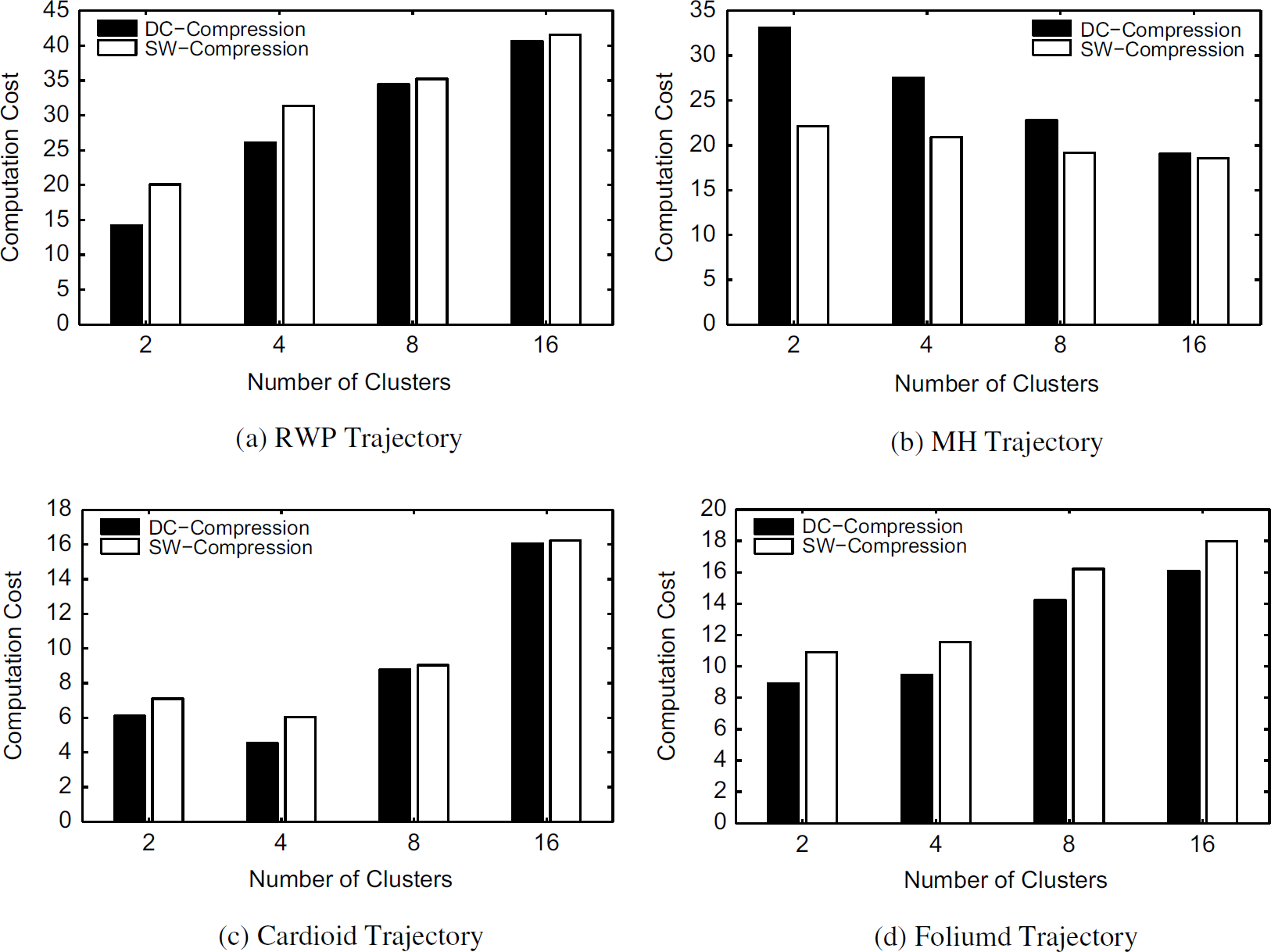
Computation cost.

5.3. Impact of Error Bound ξ

In this section, we examine the impact of error bound ξ on the performance of DTTC and DPR algorithms by varying ξ from 10m to 90m. The number of clusters used by DTTC is set to 6. Larger error bound tolerates more errors in both compressions and predictions, which intuitively leads to less communication and computation cost.

Figure 11 depicts the performance of DC-compression and DPR with linear movement trajectory. We observe from Fig. 11 (a) that prediction accuracy in DPR significantly decreases when the error bound increases, as sensor nodes tolerate more derivations between their predictions and their readings. Meanwhile, the compression accuracy in DC-compression is less affected by the error bound, due to the intelligent segmentation in DTTC. With increasing tolerance to the prediction error, both schemes show decreasing communication cost in Fig. 11 (b) for MH and RWP. Figure 11(c) shows a very interesting trend in the computation cost of DC-compression and SW-compression techniques with varying error bound. Generally, DC-compression incurs more computations (i.e., Subroutine Seg_Compression) when the error bound increases, as the compression error falls into the error bound sooner. The SW-compression is less expensive in terms of computation than the DC-compression when ξ < 50m, as fewer segments can be combined to satisfy a small error bound.

Figure 11

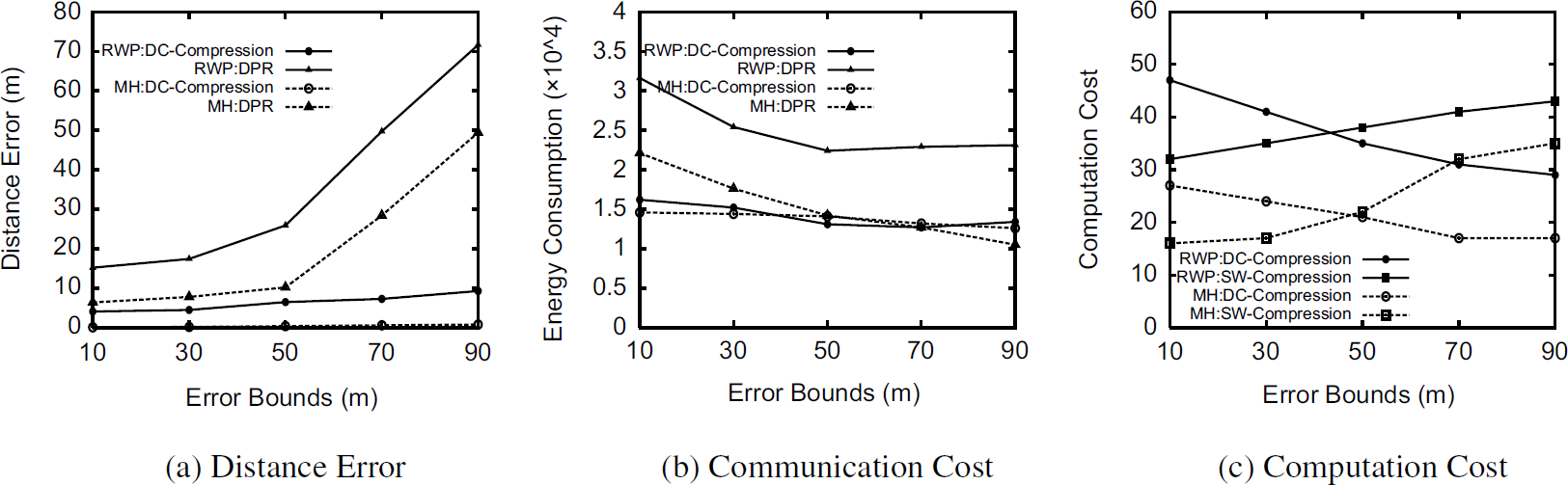
RWP and MH models.

The performance of DTTC and DPR with nonlinear trajectories (i.e., cardioid and foliumd curves), shown in Fig. 12, is similar to that with linear trajectories. Generally, DTTC and DPR both incur higher distance error with nonlinear trajectories than linear trajectory. However, as more tolerable to the compression error and prediction error, less communication costs are incurred for both schemes; DPR has a faster trend in communication reduction. We also notice that the computation cost of SW-compression increases over DC-compression very fast (e.g., error bound > 5m), while the computation cost of DC-compression decreases gradually with increasing error bound.

Figure 12

Cardioid and foliumd curves.

5.4. Impact of u

u, defined in Section 4, denotes the distance an object moves along during the period of time between two consecutive sensor reports. Intuitively, given the moving trajectory of an object, a larger u results in less sensor reports. However, this data reduction is at the cost of less accurate prediction accuracy in DPR, and compression accuracy in DTTC. u can be calculated as the product of constant moving speed and reporting duration. Moving speed indicates the moving property of an object, while the reporting duration is a parameter determined by the application. In the following, we study the impact of the above two parameters on the performance of DTTC and DPR, respectively.

We first examine the impact of moving speed on the performance of DTTC and DPR by varying the moving speed from from 4m/s to 20 m/s and fix the reporting duration as 5s. We observe from Fig. 13 (a) that the distance error of both DTTC and DPR increases when an object moves faster. For DPR, higher moving speed expands the possible moving range of an object, thus making predictions of the future movements of objects less accurate. Moreover, the faster an object moves, the more sensor nodes the object may pass through during the simulation period, which results in more historical packets and energy consumption. For DTTC, given a fixed reporting period, a cluster head receives less reports about the object's location from the nodes within its cluster, which deteriorates the compression accuracy. However, even though both schemes show increasing distance error with higher moving speed, they have a very different performance in communication cost shown in Fig. 13 (b). DPR shows a higher communication cost when the object moves faster, as prediction accuracy decreases. On the contrary, the communication cost of DTTC with foliumd trajectory gradually reduces with the increasing moving speed. This is because with the fixed length of the foliumd trajectory, less data reports from sensor nodes to the cluster heads are generated, which contributes to the communication reduction in DTTC schemes, but does not overcome the increasing communication of update packets in DPR.

Figure 13

Impact of moving speed.

Figure 14 shows the impact of reporting duration on the performance of DTTC and DPR by varying the duration from 2s to 10s with a fixed moving speed 10m/s. Intuitively, a longer reporting duration leads to a longer u, which results in less number of reports being generated by sensor nodes, but hurting the prediction and compression accuracy. Figure 14(a) verifies our intuition. The distance error of both DTTC and DPR increases when a longer reporting duration is used⁴ Moreover, we notice the total number of data reports generated in DTTC and DPR decreases, which overcomes the increasing cost of transmitting more updates packets caused by wrong predictions in DPR.

Figure 14

Impact of reporting duration.

As a summary, DTTC incurs decreasing communication cost when u increases, which is caused either by the object's faster moving speed or a longer reporting duration required by the application. This communication reduction is achieved at the cost of increasing distance error. However, DPR shows different trends to these two factors. With faster moving speed, the performance of DPR worsens in both distance error and energy cost.

6. Conclusion

The existing object tracking techniques for wireless sensor networks are designed for real-time tracking. By empowering a sink node with the ability of predicting object movements, these techniques aim at minimizing the communication cost. However, considering the complex movement patterns that an object may follow and the communication overhead a prediction-based technique involves, it is extremely difficult for existing prediction models to reach a high prediction accuracy. By reexamining object tracking applications supported by wireless sensor networks, our study proposes a novel trajectory compression technique, called DTTC, for delay-tolerant tracking in sensor networks. To the best of our knowledge, this is the first trajectory compression technique proposed for delay-tolerant object tracking sensor networks. In DTTC, each cluster head compresses the movement trajectory of a moving object by a compression function. Rather than transmitting all sensor readings to the sink node, the cluster head communicates only the compression parameters, which provides the sink node expressive yet traceable models about object movements, but also drastically reduces the total amount of data communications required for tracking operations. Moreover, aiming at minimizing the total number of segments for compression, for a given compression function, we propose two compression techniques, i.e., DC-compression and SW-compression, which favor two different movement patterns. The proposed segmentation scheme is able to wisely divide the movement trajectory into segments, which helps both the DC-compression and SW-compression techniques to compress the trajectory more accurately at less computation cost. An extensive performance evaluation is conducted to study the performance of DTTC and a prediction-based tracking technique, DPR [28]. The experimental results show that DTTC exhibits a superior performance in terms of distance error, communication cost, and computation cost, and soundly outperforms DPR with various movement trajectories. In the case of objects that frequently and abruptly change their moving direction, DTTC with SW-compression yields better results. Both the communication and computation cost could further be reduced when more clusters are employed. On the other hand, for objects that gradually change their moving direction, DTTC with DC-compression outperforms DTTC with SW-compression and clusters with medium size helps to lower the computation and communication cost.

Footnotes

1

This paper focuses on exploring energy-efficient data collection schemes for object tracking. Therefore, we only examine the closely related work in the field of data dissemination. However, similar techniques also appear in other sensor network operations, including infrastructure construction and maintenance, query propagation and etc.

2

Within each cluster, a smaller-sized tree/cluster can be used for data aggregation [16, ], which further reduces the total amount of data communication.

3

Since MH does not allow movement randomness, to be comparable, we do not consider the bumps in RWP model.

4

To be consistent and comparable, we use the default reporting duration, i.e., 5s in calculating the distance error, even though the sensor nodes do not report their readings with this duration.

Acknowledgement

Wang-Chien Lee and Yingqi Xu were supported in part by National Science Foundation grants IIS-0328881 and CNS-0626709.

References

Aslam

Butler

Constantin

Crespi

Cybenko

Rus

. Tracking a moving object with a binary sensor networks. in Proceedings of ACM SenSys, 2003, pp. 150–161.

Bai

Helmy

Sadagopan

. The important framework for analyzing the impact of mobility on performance of routing for ad hoc networks. AdHoc Networks Journal, 1, 4, 383–403, 2003.

Smart Cars and Automated Highways. http://www.memagazine.org/backissues/may98/features/smarter/smarter.html.

Coates

M. J.

. Distributed particle filtering for sensor networks. in Proceedings of International Symposium on Information Processing in Sensor Networks, 2004.

Considine

Kollios

Byers

. Approximate aggregation techniques for sensor databases. in Proceedings of International Conference on Data Engineering, Boston, MA, Mar. 2004.

Deligiannakis

Kotidis

Roussopoulos

. Compressing historical information in sensor networks. in Proceedings of ACM SIGMOD International Conference on Management of Data, France, 2004, pp. 527–538.

Estrin

Govindan

Heidemann

Kumar

. Next century challenges: Scalable coordination in sensor networks. in Proceedings of the ACM/IEEE International Conference on Mobile Computing and Networking, Seattle, Washington, August 1999, pp. 263–270.

Fang

Zhao

Guibas

. Lightweight sensing and communication protocols for target enumeration and aggregation. in Proceedings of ACM MobiHoc, pp. 165–176, 2003.

Goel

Imielinski

. Prediction-based monitoring in sensor networks: taking lessons from MPEG. ACM Computer Communication Review, 31, 5, October 2001.

10.

Guestrin

Bodik

Thibaux

Paskin

Madden

. Distributed regression: an efficient framework for modeling sensor network data. in Proceedings of IPSN, Berkeley, CA, Apr. 2004.

11.

Heinzelman

W. R.

Chandrakasan

Balakrishnan

. Energy-efficient communication protocol for wireless microsensor networks. in IEEE Proceedings of the Hawaii International Conference on System Sciences (HICSS), Maui, Hawaii, January 2000.

12.

Hill

Szewczyk

Woo

Hollar

Culler

Pister

. System architecture directions for networked sensors. ACM SIGPLAN Notices, 35, 11, 93–104, 2000.

13.

Fire Information and Rescue Information: SmokeNet Project. http://fire.me.berkeley.edu/.

14.

Ing

Coates

M. J.

. Parallel particle filters for tracking in wireless sensor networks. in Proceedings of Workshop on Signal Processing Advances in Wireless Communications, Jun. 2005.

15.

Liu

Petrovic

Zhao

. Multi-step information-directed sensor querying in distributed sensor networks. in Proceedings of International Conference on Acoustics, Speech and Signal Processing, Apr. 2003.

16.

Madden

Franklin

M. J.

Hellerstein

J. M.

Hong

. TAG: a tiny aggregation service for ad-hoc sensor networks. ACM SIGOPS Operating Systems Review, 36, SI, 131–146, 2002.

17.

Madden

S. R.

Franklin

M. J.

Hellerstein

J. M.

Hong

. The design of an acquisitional query processor for sensor networks. in Proceedings of ACM SIGMOD Conference, pp. 491–502, San Diego, CA, June 2003.

18.

Manfredi

Mahadevan

Kurose

J. F.

Lesser

. Switching kalman filtrs for prediction and tracking in adaptive meteorological sensing network. in Proceedings of IEEE Conference on Sensor and Ad Hoc Communications and Networks, 2005.

19.

Meng

Nandagopal

. Contour maps: Monitoring and diagnosis in sensor networks. Computer Networks Journal, 2006.

20.

Nath

Gibbons

P. B.

Seshan

Anderson

Z. R.

. Synopsis diffusion for robust aggregation in sensor networks. in Proceedings of ACM Sensys, Baltimore, MD, Nov. 2004, pp. 250–262.

21.

Habitat Monitoring on Great Duck Island. http://www.greatduckisland.net/.

22.

Raghunathan

Schurgers

Park

Srivastava

M. B.

. Energy aware wireless microsensor networks. IEEE Signal Processing Magazine, 19, 2, 40–50, March 2002.

23.

Ratnasamy

Karp

Shenker

Estrin

Govindan

Yin

. Data-centric storage in sensornets with GHT, a geographic hash table. Mobile Networks and Applications, 8, 4, 427–442, 2003.

24.

Sharaf

Beaver

Labrinidis

Al.

Chrysanthis

. Balancing energy efficiency and quality of aggregate data in sensor networks. The VLDB Journal, 13, 4, 384–403, 2004.

25.

Silberstein

Braynard

Yang

. Energy-efficient continuous isoline queries in sensor networks. in Proceedings of IEEE ICDE, Apr. 2006.

26.

Lee

W.-C.

. On localized prediction for power efficient object tracking in sensor networks. in Proceedings of the First International Workshop on Mobile Distributed Computing, Providence, Rhode Island, May 2003, pp. 434–439.

27.

Lee

W. C.

Mitchell

. Processing window queries in wireless sensor networks. in Proceedings of IEEE ICDE, Atlanta, GA, Apr. 2006.

28.

Winter

Lee

W.-C.

. Dual prediction-based reporting mechanism for object tracking sensor networks. in Proceedings of the International Conference on Mobile and Ubiquitous Systems: Networking and Services, Boston, MA, Aug. 2004, pp. 154–163.

29.

Winter

Lee

W.-C.

. Prediction-based strategies for energy saving in object tracking sensor networks. in Proceedings of the International Conference on Mobile Data Management, Berkely, CA, Jan. 2004, pp. 346–357.

30.

The ZebraNet Wildlife Tracker. Princeton university. http://www.princeton.edu/mrm/zebranet.html.

31.

Zhao

Shin

Reich

. Information-driven dynamic sensor collaboration for tracking applications. IEEE Signal Processing Magazine, 19, 2, 61–72, March 2002.

Compressing Moving Object Trajectory in Wireless Sensor Networks

Abstract

Keywords

1. Introduction

2. Related Work

2.1. Suppression and Prediction

2.2. Aggregation

3. Design of Delay-Tolerant Trajectory Compression

3.1. Basic Idea of DTTC

3.3.1 DC-Compression

5.1. Simulation Settings

Footnotes

1

2

3

4

Acknowledgement

References