Sage Journals: Discover world-class research

Abstract

Networked Embedded Systems have come to occupy an important role in emerging applications. Nodes in such a system are interconnected by a mesh topology. Despite the availability of multiple shortest paths between pairs of nodes, simulation results revealed that these paths cannot be effectively exploited by spreading the messages over the paths in a uniform method. We define the union of all the shortest paths between a pair of nodes as a contour. We present results that characterize the structure of contours when each node communicates directly with eight immediate neighbors. Heuristic rules that effectively disseminate messages over the available paths are presented. Simulation results demonstrate that the new method for dissemination ensures that nodes in a contour, which are at the same distance from the source, handle roughly the same number of messages. In the future, such techniques can be extended to general topologies.

Keywords

Multipath Dissemination QoS Wireless Communication Routing Protocols Mesh Topology

1. Introduction

Networked embedded systems have emerged as a platform with tremendous capabilities and opportunities for future engineered systems. Such a platform comprises a large number of tiny, resource-constrained microcontroller nodes that have limited capabilities for computation and communication [1]. Sensor networks [2, 3] and networked sensor-actuator systems (NSAS) [4] are two examples of networked embedded systems. This paper presents a novel approach for dissemination in networked embedded systems called Contour Guided Dissemination (CGD) [5].

The problem of disseminating messages in networked embedded systems is particularly challenging because of the resource constraints at the node-level, limited bandwidth, high bit-error rates, and irregular propagation of the wireless links [6]. Because the wireless medium has a relatively low bandwidth, it is not desirable for every node to communicate with every other node directly. The immense scale makes it infeasible to associate a network address with each node in a networked embedded system. Propagation of messages between non-neighboring nodes without relying on unique network identifiers for each node, is referred to as dissemination in the sensor network literature [7]. This investigation considered the problem of disseminating the messages from a source node to a sink node when the nodes of a networked embedded system are located on a two-dimensional grid. A new method for dissemination that exploits the location of each node and multiple paths between nodes is presented.

Methods to disseminate messages from a source to one or more sink nodes have been addressed in the networking literature. Traditionally, routing protocols that are based on shortest-path algorithms such as the Bellman-Ford algorithm [8] and Dijkstra's algorithm [9] are the basis for these methods. For example, distance vector routing and link-state routing are two well-known protocols that are used in distributed systems [10, 11]. The distance vector routing protocol, which is based on the Bellman-Ford algorithm, requires each node to maintain a routing table. Each entry in the routing table of a node identifies the next node to which, a packet destined for a sink, must be sent. If d(i, snk) represents the distance from node n_i to the sink node, and n_j is a neighbor of n_i, then the routing table of n_i is updated for a neighbor n_j whenever d(i, snk) > d(j, snk) + d(i,j), i.e., whenever a node discovers a new, shorter, route to the sink. In order to maintain accuracy of the routing tables, each node must notify its neighbors whenever its own routing table changes.

In addition to the message overheads, approaches based on the above algorithms are not suitable for sensor networks and networked embedded system. For example, when the topology is disrupted because of faults, it takes a long time for the routing tables in each node to converge to a stable state. The node resources are constrained and hence, it is not desirable to store and maintain routing tables. When there are multiple monitoring stations, every node must maintain a routing table for every monitoring station. Routing methods that are based on shortest path algorithms select a single path from a node to a sink. Because all the message propagates along this path, the nodes along this path must have more resources than other nodes in the networked embedded system.

In many engineered systems, the nodes are located at well-designed, fixed, locations. For example, in automotive assembly lines or warehouse conveyor systems, every module is located in a zone. Further, to ensure that the system is robust, multiple paths for communication between a pair of nodes are designed into the system. The motivating question for this investigation was whether all the available paths between a pair of nodes can be effectively used to disseminate messages.

1.1. Overview

Section 2 describes the monitoring problem, which is one application for Contour Guided Dissemination. Section 3 presents the Contour Guided Dissemination method. After defining the contour as the union of all shortest paths between a pair of nodes, it is shown that the relative locations of nodes are necessary and sufficient to allow each node to determine its position in a contour. Next, it is shown that to benefit from the multiple paths in a contour, it is not sufficient to uniformly spread the messages among the available paths; surprisingly, one path in the contour gets loaded with more messages than the other paths. A heuristic that efficiently spreads the messages over the available paths is presented. Section 4 presents the simulation results and Section 5 presents the conclusions.

2. Background

The problem of sending messages from a source over a multi-hop path is related to routing in wired and wireless networks [12] and to data dissemination in sensor networks [2] These approaches aim to move data from one or more sources to one or more sinks over a multi-hop network.

The two dominant methods used in wired networks are the distance vector scheme and the link state scheme that are based on the shortest path algorithms by Bellman [8] and Dijkstra [9], respectively, as discussed briefly in Section 1 Contour Guided Dissemination departs from the application-specific methods advocated in the sensor networks literature [7].

Networked embedded systems have unique characteristics such as scale, constrained resources, unreliable channel, and unpredictable failures. It is necessary to consider that the execution is periodic and may be based either on an event-triggered or time-triggered model. Nodes are not deployed in an ad-hoc manner and the geometric structure of the nodes can be exploited. The “query-response” model [13] is useful for networked embedded systems—however, the “queries” are not ad hoc; in contrast, they are highly structured; queries are issued infrequently in response to faults that occur in the environment.

2.1. Dissemination Protocols

Flooding and Gossiping [14] are two data centric schemes for propagating data in multi-hop networks. These schemes are called data-centric because the propagation is not based on the address, or any other identifier, of the nodes involved in the propagation. In flooding, a node forwards its data to all its neighbors; note, that in a wireless network, this effect can be achieved by a single broadcast. In Gossiping, a node forwards data to a neighbor that is selected at random; once again, note that since broadcast is the primary mode of communication in a wireless medium, the neighboring nodes that are “not-selected” must drop the data. A protocol called SPIN [11] uses meta-data to reduce the data traffic in a sensor network. In this approach, a node advertises the data it has and only sends the data only if a neighbor requests the data.

Reverse-path forwarding [7] is a general approach that is used in several dissemination protocols. In this approach, a sink node (such as a Monitoring Station) generates a “query” that indicates an interest in data items from one or more nodes. Such a query is forwarded along one or more paths from the sink to all the nodes. The nodes forward data along these paths; since the data propagates in a direction that is reverse of the query direction, this method is referred to as reverse-path forwarding. Declarative routing protocol (DRP [15]), Directed Diffusion (DD [16]) and resilient multiple path Directed Diffusion [17] are examples that are based in reverse-path forwarding.

Cost field approach is another choice for routing. Every node maintains a scalar that represents the cost of sending data back to the sink and the data is propagating along the cost gradients. In [13] paper, the cost field approach is divided into two categories: the receiver-decided protocols and the sender-appointed protocols. Protocols based in cost-field require less memory space compared to reverse-path forwarding since there is no need to maintain a routing table. Routing decisions are based in the cost at each node. Since nodes are resource constrained in both communication and computation capabilities, the cost field based approach is a good choice.

GRAdient routing in Ad Hoc network (GRAd), simple cost field protocol [18], and GRA-dient Broadcast (GRAB [19]) are examples of a receiver-decided protocol. First, the sink floods the network with the request message and sets up scalar values. For examples, if a node receives from a node which has N hops to the sink, then it will set up its own scalar as N + 1 hops to the sink. Energy Aware Routing(EAR [20]) and CGD discussed in this paper are examples of sender-appointed protocols. The sender computes the cost of sending the data along the multiple paths depending on the location of the sink, and then chooses the least cost route to send its messages back to the sink.

Virtual hierarchy approach: This approach achieves scalability by applying multiple levels in the network. As shown in Fig. 1, the nodes form local clusters and a cluster head will be elected from the cluster. Nodes in the cluster may rotate their roles as the cluster head in order to achieve the energy consumption balance in the cluster. Since the radio transmission strength is adjustable, the cluster head node can be set to a more powerful transmission range to reach the monitoring station. Low-energy adaptive clustering hierarchy (LEACH [21]) and Adaptive Threshold sensitive Energy Efficient sensor Network (APTEEN [22]) are examples of such protocols.

Geographical forwarding: By utilizing the GPS or the location on a grid, the network uses location information to achieve a more efficient routing in the network. Geographic adaptive fidelity (GAF [23]) sets up a virtual grid depending on the GPS providing location and saves energy in the network by propagating messages in different nodes in the same region. Geographical and Energy Aware Routing (GEAR [24]) reduces traffic load by first sending a beacon in a sub region which the sink is interested in and then disseminate the query into this region.

Routing on a curve is an interesting generalization of source based routing and Cartesian routing suitable for dense sensor networks [25]. In this approach, route paths are modeled as continuous functions. In contrast, the CGD method proposed here is a sender-appointed routing scheme that effectively exploits all the shortest paths between a pair of nodes.

Real-time delivery and QoS: the protocols in the category consider the useful life time of a packet and try to send the message back to the sink before the useful life time expires. RAP [26] achieves this by adjusting the packet priority in the queue, backoff and waiting parameters in the MAC layer. SPEED [27] calculates the distance, D, between the node with a message and the sink and dividing by the life time, t. After getting the velocity $v = \frac{D}{t}$ , the message is forwarded to the sink.

In network data-processing: Instead of sending all the measured data back to the sink, the local nodes will process the data and only sends out a summary to the sink. Sensor Protocols for Information via Negotiation (SPIN [28]) and directed diffusion belong to this field. No matter in what kind of network, reducing the redundant traffic in the network is always preferred.

Figure 1.

Hierarchical approach for routing.

Table 1 shows a summary of the dissemination protocols discussed in this section. Add on features such as QoS, virtual hierarchy, etc., can be integrated into both reverse-path forwarding and cost-field approach.

TABLE 1

Protocols Comparison

		Cost field based approach			Multiple Path		Add-on features
	Reverse Path Forwarding	Sender appointed	Receiver decided	Single path	Load balancing	No load balancing	OoS	Virtual hierarchy	Location-based	In-network processing	Data-centric
FWDE						x				x
Gossiping						x
DD	x			x						x	x
DRP	x			x
GRAd			x			x
GRAB			x		x
EAR		x		x
CGD-1		x				x			x
ODS
CGD-2		x			x				x
WDS
CGD-3		x			x				x
HDS
LEACH	Add-on							x
SPIN	Add-on									x	x
GEAR	Add-on							x	x
RAP	Add-on						x
SPEED	Add-on						x
APTEEN	Add-on							x
GAF	Add-on								x
SAR	Add-on						x

2.2. Coupled Conveyors

Coupled Conveyors is a method for building conveyor systems with an integrated networked embedded system that regulates its operations. The conveyor systems are assembled using three building blocks called Segment, Turnaround, and Crossover [4]. The following are two examples from [4].

2.3. Example 1: Inspection Station

Consider the instance of coupled conveyors shown in Fig. 2. This instance represents an application of coupled conveyors for material inspection and/or sorting. There are 18 Segments, 4 Turnarounds, and one Crossover in this instance. The module identities are shown next to each module. For example, port D of Turnaround T₄ is embedded at grid location (1,1), and port A of Turnaround T₂ is at grid location (5,3). Crossover C₁ is at grid location (3,3); HCI devices H₁, H₂, and H₃ are at grid locations (1,0), (3,4), and (5,0), respectively. All the other modules are embedded with appropriate directions as shown in Fig. 2¹.

Figure 2.

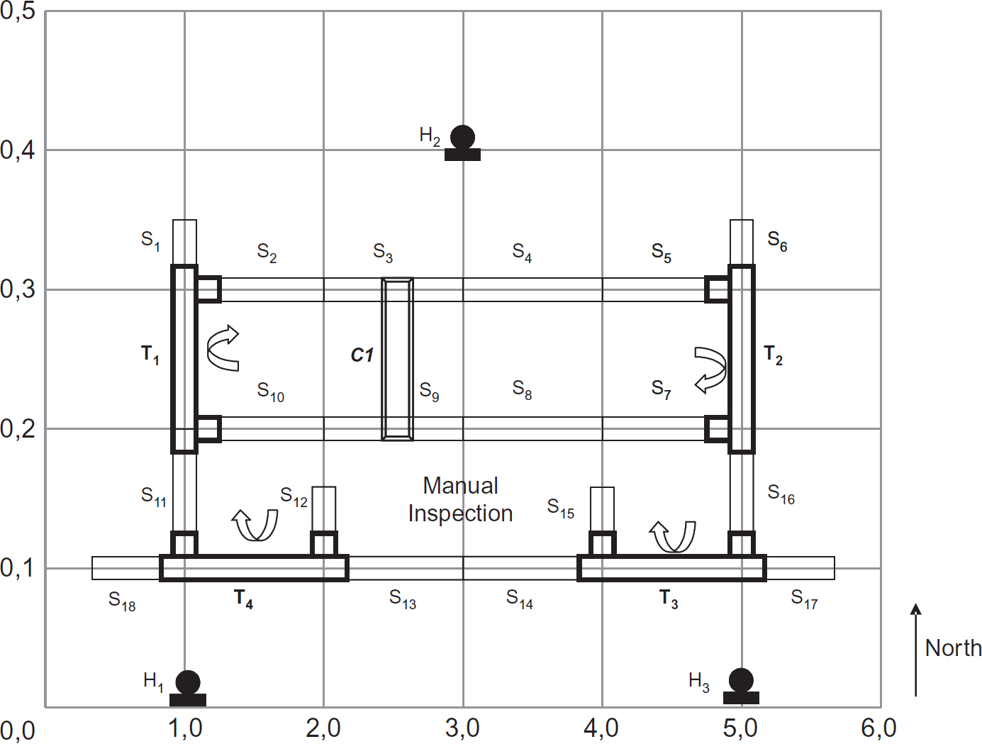
An inspection system.

Entities come in to the system via S₆ (at port A of T₂) or S₁₇ (port A of T₃). Entities leave the system via port D of T₄ or via S₁ (at port D of T₁). Entities coming in via S₆ may be moved either along the path

T_{2}, S_{7}, S_{8}, S_{9}, S_{10}, T_{1}, S_{1}

or along the path

T_{2}, S_{16}, T_{3}, S_{14}, S_{13}, T_{4}, S_{11}, T_{1}, S_{1} .

Entities may be deflected for re-inspection via port C of T₃. Defective or oversized material that are likely to damage the inspection devices along the subpath S₁₀, T₁ may be diverted using C₁. Entities coming into T₃ can be moved along the subpath T₃, S₁₄, S₁₅, or deflected at port C of T₃ for manual inspection. Manually inspected entities may be reinserted into the system via port B of T₄. The HCI devices are used to monitor the status of all modules and the operator panels can be used to issue commands such as start, stop, or force manual inspection for all entities over a duration of time. There are several other possibilities for moving entities in coupled conveyors that are not discussed in the examples in this paper.

2.4. The Monitoring Problem

Consider a typical engineered system that is depicted in Fig. 3. All the operations of this system are regulated by controllers and monitoring stations are directly connected to these controllers [29]. Periodically, the controllers send a block of words to the monitoring stations to update status. Systems software executing in the monitoring stations translate such a block of words to graphical widgets that are presented to users.

Figure 3.

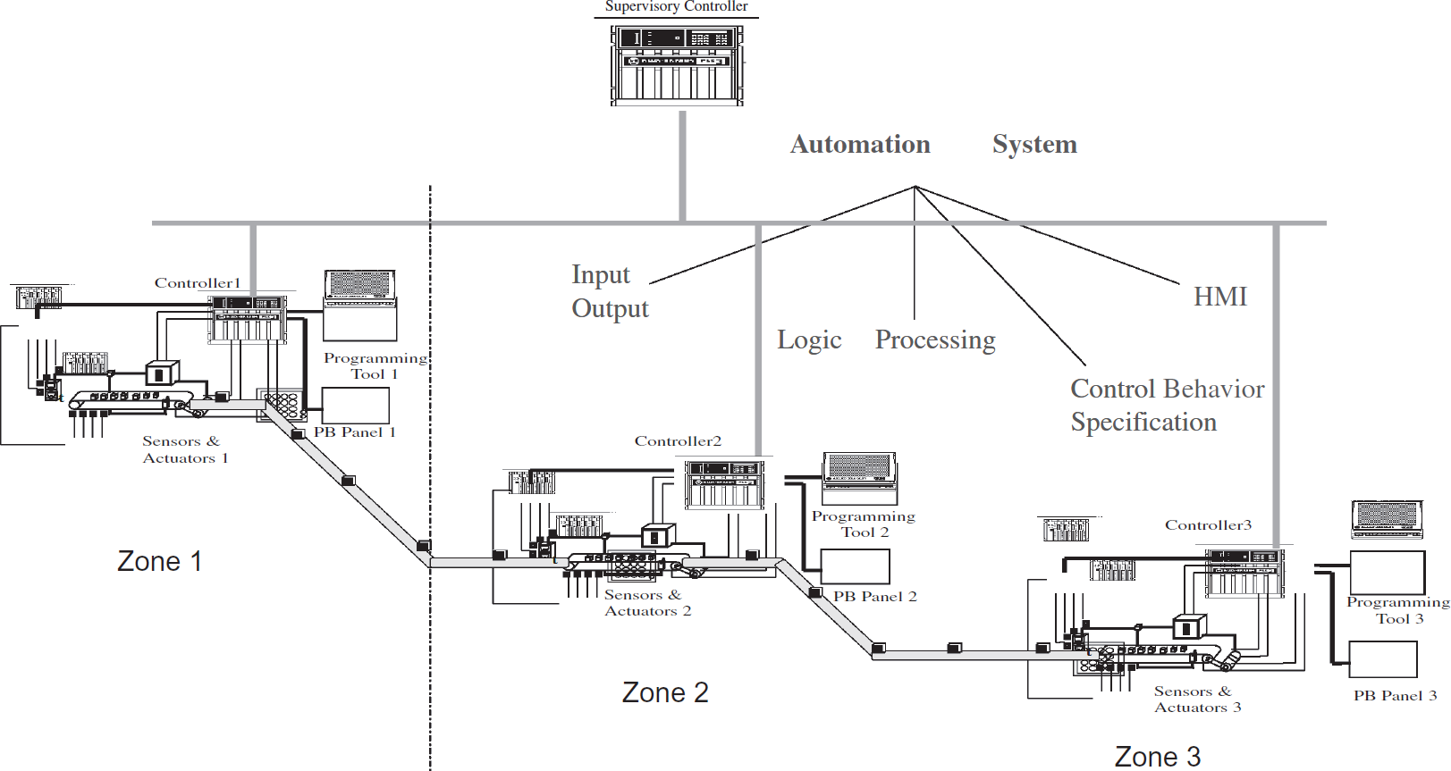
Monitoring in automation systems.

Consider an networked embedded system as shown in Fig. 4. In this system StatusMessages are delivered to monitoring stations over multi-hop routes. Consider four nodes n₁,₁, n_1,2, n_1,3, and n_1,4 and a monitoring station M1. Only node n_1,1 can communicate with M1 in one hop. Let $m_{i, j}^{k}$ denote the status message generated by segment n_i,j in time tick k. The multi-hop delivery of StatusMessages in this scenario is shown in Table 2.

TABLE 2

Multi-hop Delivery Scenario 1

Time	M1	n _1,1	n _1,2	n _1,3	n _1,4
1		$m_{1, 1}^{1}$	$m_{1, 2}^{1}$	$m_{1, 3}^{1}$	$m_{1, 4}^{1}$
2	$m_{1, 1}^{1}$	$m_{1, 2}^{1} m_{1, 1}^{2}$	$m_{1, 3}^{1} m_{1, 2}^{2}$	$m_{1, 4}^{1} m_{1, 3}^{2}$	$m_{1, 4}^{2}$
3	$m_{1, 1}^{2} m_{1, 2}^{1}$	$m_{1, 3}^{1} m_{1, 2}^{2} m_{1, 1}^{3}$	$m_{1, 4}^{1} m_{1, 3}^{2} m_{1, 2}^{3}$	$m_{1, 4}^{2} m_{1, 3}^{3}$	$m_{1, 4}^{3}$
4	$m_{1, 1}^{3} m_{1, 2}^{2} m_{1, 3}^{1}$	$m_{1, 4}^{1} m_{1, 3}^{2} m_{1, 2}^{3} m_{1, 1}^{4}$	$m_{1, 4}^{2} m_{1, 3}^{3} m_{1, 2}^{4}$	$m_{1, 4}^{3} m_{1, 3}^{4}$	$m_{1, 4}^{4}$
5	$m_{1, 1}^{4} m_{1, 2}^{3} m_{1, 3}^{2} m_{1, 4}^{1}$	$m_{1, 4}^{2} m_{1, 3}^{3} m_{1, 2}^{4} m_{1, 1}^{5}$	$m_{1, 4}^{3} m_{1, 3}^{4} m_{1, 2}^{5}$	$m_{1, 4}^{4} m_{1, 3}^{5}$	$m_{1, 4}^{5}$
6	$m_{1, 1}^{5} m_{1, 2}^{4} m_{1, 3}^{3} m_{1, 4}^{2}$	$m_{1, 2}^{5} m_{1, 3}^{4} m_{1, 4}^{3} m_{1, 1}^{6}$	$m_{1, 4}^{4} m_{1, 3}^{5} m_{1, 2}^{6}$	$m_{1, 4}^{5} m_{1, 3}^{6}$	$m_{1, 4}^{6}$

Figure 4.

Monitoring an networked embedded system.

Generalizing the phenomenon in Table 2 and Fig. 4, if

P =< v_{1}, v_{2}, . . ., v_{n} >= M_{i}

is a longest path in the networked embedded system that terminates in some monitoring station, node v_i in P must maintain a buffer of size n - i to store and forward StatusMessages from its preceding nodes in the path.

2.5. Challenges for Monitoring

Networked embedded system nodes are not energy-constrained. However, these nodes are severely resource-constrained. These constraints are desirable to ensure easy scalability and maintenance. Consequently, large buffers cannot be maintained at each node. In addition, the node can only perform limited computation and communication. When the computation load is increased, the capacity for communication, sensing, and actuation is decreased. Communication rates can also not be increased because of the performance of the Media Access Control (MAC) protocol.

Carrier Sensing Multiple Access (CSMA) with Collision Avoidance is a basic MAC protocol that is used in sensor networks. Figure 5 shows the performance of CSMA as the number of nodes contending for the channel increases and as the rate at which the nodes initiate communication messages is increased. It can be noticed that when the rate increases, the number of messages received without collisions significantly drops. The number of messages received also decreases when the number of nodes contending for the channel increases. To address these challenges, the approach used here aimed to exploit multiple paths that are available between a pair of nodes.

Figure 5.

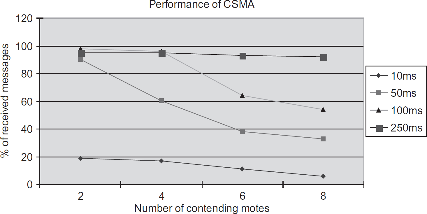
Performance of CSMA.

3. Contour Guided Dissemination

A contour is the union of all the shortest paths between a pair of nodes. Every node is either in the contour or not; only nodes in the contour participate in the dissemination. Section 3.1 develops results that are sufficient to allow each node to compute its own position on a contour using local computations. It was intuitively appealing to utilize the multiple paths in a contour by uniformly spreading the messages over the available paths. It is shown that this intuitive idea results in one path being loaded, despite the availability of multiple paths. A heuristic spreading method that effectively uses the multiple paths is presented.

3.1. Contour of Shortest Paths

Consider an networked embedded system in which each node n_i,j is located at on a grid. Each node can communicate directly with its eight immediate neighbors² as shown in Fig. 6. Because such communication is possible, there exist multiple shortest paths between any a pair of nodes, n_i,j and n_q,r, in the grid.

Figure 6.

Eight neighbors of a node n_i,j

Definition 1

The contour of the shortest paths between n_i,j and n_q,r (“contour of n_i,j and n_q,r” for short) is the union of all the shortest paths between n_i,j and n_q,r. Each path in the contour is different from every other path by at least one edge.

Definition 2

Given a pair of nodes n_i,j and n_q,r,

\begin{aligned} x_{d i f f} (n_{i, j}, n_{q, r}) = | q - i |, \\ y_{d i f f} (n_{i, j}, n_{q, r}) = | r - j |, \\ x y_{d i f f} (n_{i, j}, n_{q, r}) = | x_{d i f f} (n_{i, j}, n_{q, r}) - y_{d i f f} (n_{i, j}, n_{q, r}) |, a n d \\ κ (n_{i j}, n_{q r}) = ⌊ \frac{x y_{d i f f}}{2} ⌋ . \end{aligned}

When the context is clear, x_diff, y_diff, xy_diff and κ are used without explicitly specifying the nodes.

Observation 1

The length of the shortest path between nodes n_i,j and n_q,r is max(x_diff, y_diff).

Proof

Follows from the structure of the grid.

Lemma 1

Let y_diff = 0. Given a pair of nodes n_i,j and n_q,r, the contour of n_i,j and n_q,j is a rectangle, with corner nodes n_i,j, n_{i + κ, j − κ}, n_{q− κ, j + κ}, and n_q,j, if and only if x_diff is even.

Proof

First, given y_diff = 0 and x_diff is even, it is shown that the four corner nodes of the contour are n_i,j, n_i+κ,j-κ, n_q-κ,j+κ, and n_q,j. Consider the shortest paths shown in Fig. 7. The obvious shortest path between the nodes n_i,j and n_q,j is along the path <n_i,j, n_i+1,j, …, n_q-1,j, n_q,j=r>. Since x_diff is even, there are an odd number of nodes in the path. Let us call this path a Layer 0 path for convenience. As shown in Fig. 7, there are additional shortest paths between the nodes n_i,j and n_q,r Any subpath < … n_s,t,n_s+1,t,n_s+2,t, … > can be replaced by a path < … n_s,t,n_s+1,t+1,n_s+2,t, … > or < … n_s,t,n_s+1,t-1,n_s+2,t, … > without increasing the length of the shortest path. However, in Layer 1, the node n_i,j+1 cannot be on any shortest path because any path between n_i,j and n_q,j that passes through n_i,j+1 must be of length ≥ x_diff + 1. Similarly, node n_q,j+1 (in Layer 1) cannot be on any shortest path.

Figure 7.

Layered paths when x_diff is even.

It may be noticed that in each layer, p, 1 ≤ p ≤ κ, the number of nodes that can appear on any shortest path between n_i,j and n_q,j is decreased by 2 × p. Since Layer 0 has an odd number of nodes, Layer κ must have a single node, i.e., n_i+κ,j+κ which is one corner node. Using similar arguments, it is noticed that there are additional shortest paths between n_i,j and n_q,j that go through nodes in Layers −1, −2, …, -κ. Once again, Layer -κ must have a single node, i.e., n_i+κ,j-κ. Since x_diff is even and y_diff = 0, q − κ = i + κ, the four corner nodes of the rectangle are specified in the Lemma.

Next, given y_diff = 0 and a contour with four corner nodes n_i,j, n_i+κ,j-κ, n_{q −
κ,j+κ} and n_q,j, it is shown that x_diff is even.

Consider the path from n_i,j to n_i+κ,j+κ. The length of this path is the same as the length of the path from n_i,j to n_i+κj because of the structure of the grid. It follows from the construction that x_diff is 2 × κ and hence must be even. □

Lemma 2

Let x_diff = 0. Given a pair of nodes n_i,j and n_q,r, the contour of n_i,j and n_q,j is a rectangle, with corner nodes n_i,j, n_i-κ,j+κ, n_{i+κ j+κ} and n_i,r, if and only if y_diff is even.

Proof

Similar to the proof of Lemma 1, except that the Layer 0 path will be along the y axis. □

Lemma 3

Let y_diff = 0. Given a pair of nodes n_i,j and n_q,r, the contour of n_i,j and n_q,j is a hexagon, with corner nodes n_i,j, n_i+κ,j-κ, n_i+κ+1,j-κ, n_q-κ,j+κ, n_{q-κ−1,j+κ} and n_q,j, if and only if x_diff is odd and x_diff ≥ 3.

Proof

Consider the shortest paths between node n_i,j, and n_q,j, when y_diff = 0 and x_diff is odd, as shown in Fig. 8. The arguments are similar to the proof of Lemma 1. Because x_diff is odd, there are an even number of nodes along the path involving only the nodes in Layer 0. As in the case of Lemma 1, the number of nodes that can be on any shortest path in Layer p, 1 ≤ p ≤ κ, decreases by 2 × p compared to the number of nodes in Layer 0. However, since the Layer 0 path has an even number of nodes, Layer κ must have two nodes, i.e., n_i+κ,j+κ and n_i+κ+1,j+κ. Similarly, Layer -κ will have the two nodes n_i+κ,j-κ and n_i+κ+1,j-κ.

Figure 8.

Layered paths when x_diff is odd.

Given y_diff = 0 and a contour with six corner nodes n_i,j, n_i+κ,j-κ, n_i+κ+1,j-κ, n_q-κ,j+κ, n_{q-κ−1,j+κ} and n_q,j, Consider the path from n_i,j to n_i+κ,j+κ. The length of this path is the same as the length of the path from n_i,j to n_i,j+κ and the path from n_q,j to n_q-κ,j+κ is the same as the length of the path from n_q,j to n_q-κ,j. Because of the structure of the grid, x_diff is 2 × κ + 1 and hence must be odd. □

Lemma 4

Let x_diff = 0. Given a pair of nodes n_i,j and n_q,r, the contour of n_i,j and n_i,r is a hexagon, with corner nodes n_i,j, n_i-κ,j+κ, n_i-κ,j+κ+1, n_{i + κ,r-κ}, n_{i+κ,r-κ−1} and n_i,r, if and only if x_diff is odd and y_diff ≥ 3.

Proof

Similar to the proof of Lemma 3. □

Theorem 1

The contour of n_i,j and n_q,r is a rectangle bounded by the nodes n_i,j, n_i+κ,j-κ, n_q-κ,r+κ and n_q,r if and only if xy_diff is even.

Proof

Given that xy_diff is even, either both x_diff and y_diff are even or both x_diff and y_diff are odd. Without loss of generality, assume that x_diff > y_diff. Two such nodes are shown in Fig. 9.

Figure 9.

Contour when xy_diff is even.

Consider the case when both x_diff and y_diff are odd. Consider the shortest path from node n_q-r+j,j to n_q,r. Clearly, no shortest path between these nodes can pass through the node n_q,j. In fact, the shortest path is via the node n_q-r+j+1,j+1, n_q-r+j+2,j+2 to n_q,r. Because y_diff is odd, the path from n_i,j to n_q-r+j,j must be even and the conditions of Lemma 1 apply. Consequently, the contour of n_i,j and n_q-r+j,j is a rectangle. Since the length of the path from n_i,j to n_q-r+j,j is xy_diff, by definition, the corner nodes of this rectangle are n_i,j, n_i+κ,j-κ, n_i+κ,j+κ and n_q-r+j,j. Hence, nodes n_i,j and n_i+κ,j-κ are at least two corner nodes of the rectangle.

Next, consider the path n_i,j, n_i+1,j+1…n_i+r-j,r. Because the nodes can communicate across the diagonal links, this path must be on a shortest path from n_i,j to n_q,r. Further, since y_diff is odd, the path from n_i+r-j,r to n_q,r via the nodes n_i+r-j+1,r, n_i+r-j+2,r to n_q-1,r, n_q,r must be even. Hence, by Lemma 1, the contour of n_i+r,q+r and n_q,r is a rectangle. Since the length of the path from n_i+r-j,r to n_q,r is by definition xy_diff, the remaining two corner nodes of this contour are n_{i+r-j+κ,r+κ} and n_{i+r-j+κ,r-κ}. Since xy_diff to the source and the sink nodes are both 0, they are corner nodes.

The arguments when xy_diff is even and both x_diff and y_diff are even are similar to the above arguments. Since n_{i+r-j+κ,r+κ} is the same as n_q-κ,r+κ, when xy_diff is even, the contour of n_i,j and n_q,r is a rectangle that is bound by the four nodes n_i,j, n_i+κ,j-κ, n_q-κ,r+κ and n_q,r.

Next, given a contour of n_i,j and n_q,r with four corner nodes as n_i,j, n_i+κ,j-κ, n_q-κ,r+κ and n_q,r, it is shown that xy_diff of n_i,j and n_q,r must be even.

xy_diff (n_i,j, n_q,r) is even only when x_diff (n_i,j, n_q,r) and y_diff (n_i,j, n_q,r) are both even or are both odd. By definition, $k (n_{i, j,} n_{q, r}) = \frac{| q - i | - | r - j |}{2}$ , and $k (n_{i, j,} n_{q - r + j . j}) = \frac{| (q - r + j) - i | - | j - j |}{2}$ . Thus, k(n_i,j, n_q,r) = k(n_i,j, n_q-r+j,j). n_i+k,j-k is a corner node in the contour of n_i,j and n_q-r+j,j. x_diff(n_i,j, n_q-r+j+r) = 2 × k (n_i,j, n_q-r+j,j) by the structure of the grid and hence is even by Lemma1. xy_diff(n_i,j, n_q-r+j,r) = 0, hence, the distance d(n_q-r+j,j, n_q,j) is always equal to d(n_q,r, n_q,j). Therefore, x_diff(n_i,j, n_q,r) and y_diff(n_i,j, n_q,r) are either both even or both odd. Hence, xy_diff(n_i,j, n_q,r) must be even. □

Observation 2

When xy_diff = 0, the four nodes that bound the rectangle in Theorem 1 are n_i,j, n_i+0,j−0, n_q−0,_r+0 and q, r; i.e., the shortest path between nodes n_i,j and n_q,r is unique and the contour of n_i,j and n_q,r contains only this path.

Theorem 2

The contour of n_i,j and n_q,r is a hexagon bounded by the nodess n_i,j, n_i+k,j-k, n_i+k+1,j-k, n_q-k,r+k, n_q-k-1,r+k and (q, r) if and only if xy_diff is odd and xy_diff ≥ 3.

Proof

The proof is very similar to the proof of Theorem 1. □

Observation 3

When xy_diff = 1, κ = 0 and hence, the six corner nodes that bound the hexagon in Theorem 2 are n_i,j, n_i+0,j−0, n_i+0+1,j−0, n_{q−0, r+0}, n_{q−0−1,
r+0} and n_q,r; i.e., the corner nodes of the contour are n_i,j, n_i+1,j, n_q,r and n_q−1,r.

Observation 4

Every node in the contour of n_i,j and n_q,r will have one two or three shortest paths to n_q,r.

Proof

Proof is immediate from the construction of the contour.

The results in this section are used by networked embedded system nodes to compute the contour.

3.2. Uniform Spreading

Assume that a node (source) is sending messages to a sink such as a monitoring station. Every message contains the location of the source and the sink³.

Figure 10 depicts a scenario when the source is sending 99 messages to the sink. Every node in the contour uniformly spreads all the messages it receives over all the shortest paths from itself to the sink. Because xy_diff is even, the contour is a rectangle. The number in each node represents the number of messages that are handled by the node. As may be noticed in Fig. 10, the nodes close to the top left diagonal edge of the contour have many more messages than the other nodes.

Figure 10.

Uniform spreading.

Observation 5

A series of simulations using uniform spreading revealed that the nodes along one path in the contour always handled more messages than the other paths.

3.3. Orientations of a Contour

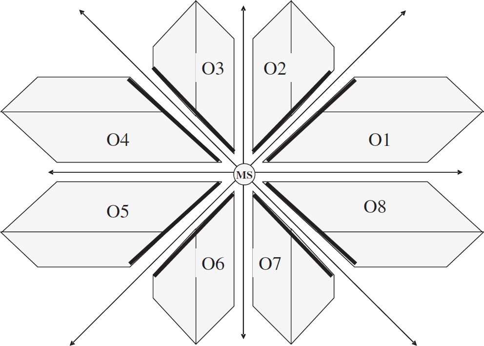
Figure 11 shows a monitoring station located at the center. The plane is divided into eight octants. For convenience, the octants are named O1, O2, …, O8 in the counterclockwise direction as shown.

Figure 11.

Orientations of a contour.

When xy_diff = 0, the source node will lie on one of the diagonal lines and the contour comprises a single path (Lemma 1). When x_diff = 0 and y_diff ≠ 0, or y_diff = 0 and x_diff ≠ 0, the contour will be symmetrical around the non-zero axes. In all other cases, most of the shortest paths in the contour lie in the same octant as the one in which the source node is located.

Definition 3

When xy_diff ≠ 0, or x_diff ≠ 0, y_diff ≠ 0, the orientation of a contour is the number of the octant in which the source node is located.

The right side of Fig. 11 shows a contour with Orientation 1. Most of the shortest paths in this contour lie in octant 1.

It was observed through simulations that when the orientation of the contour is 1, nodes on the path closer to the diagonal line always handle more messages then the other nodes in the contour. The nodes that appear in the light colored area in Fig. 11 handle most of the messages. Further, irrespective of the orientation of the contour, nodes on the path closest to the diagonal lines, which divide the plane into octants, always handle more messages than other nodes in the contour. Figure 12 shows the contour in eight possible orientations⁴. The solid lines in Fig. 12 depict the paths on which nodes that handle most messages are located.

Figure 12.

Eight possible orientations for contours.

Let ${\hat{x}}_{d i f f}, {\hat{y}}_{d i f f}$ and $\hat{x} y_{d i f f}$ represent the values of x_diff, y_diff and xy_diff, respectively, when the sign is also considered. Table 3 shows the conditions necessary for a contour to have one of the eight orientations.

TABLE 3

Orientation Conditions

Orientation	x _diff	y _diff	xy _diff
1	> 0	< 0	> 0
2	> 0	< 0	< 0
3	< 0	< 0	< 0
4	< 0	< 0	> 0
5	< 0	> 0	> 0
6	< 0	> 0	< 0
7	> 0	> 0	< 0
8	> 0	> 0	> 0

3.4. Heuristic Spreading

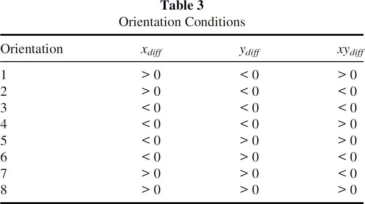
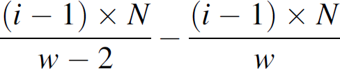
Based on the above simulation observations, methods to effectively spread the messages over the available paths in a contour were explored. The theorems from Section 3.1 were used by each node to compute the contour. The heuristic method for spreading depends on recognizing that each node can also compute the width, w of the contour at its own location because it knows the distance from itself to the source and the sink and all the corner nodes of the contour. When the messages are spread ideally, each node will handle $\frac{N}{w}$ messages, where N is the number of messages that must be sent from the source to the sink, as shown in Fig. 13.

Figure 13.

Ideal messages loading in the contour.

As shown in Fig. 14, starting from the source, messages must be spread only for the first κ steps. After κ steps, the nodes select one shortest path towards the sink and not spread the messages as long as the number of nodes at the next step is equal to the number of the nodes in the current step. The nodes within κ steps from the sink must aggregate messages from the nodes in the preceding step. The theorems in section 3.1 used by the node to determine the contour.

Figure 14.

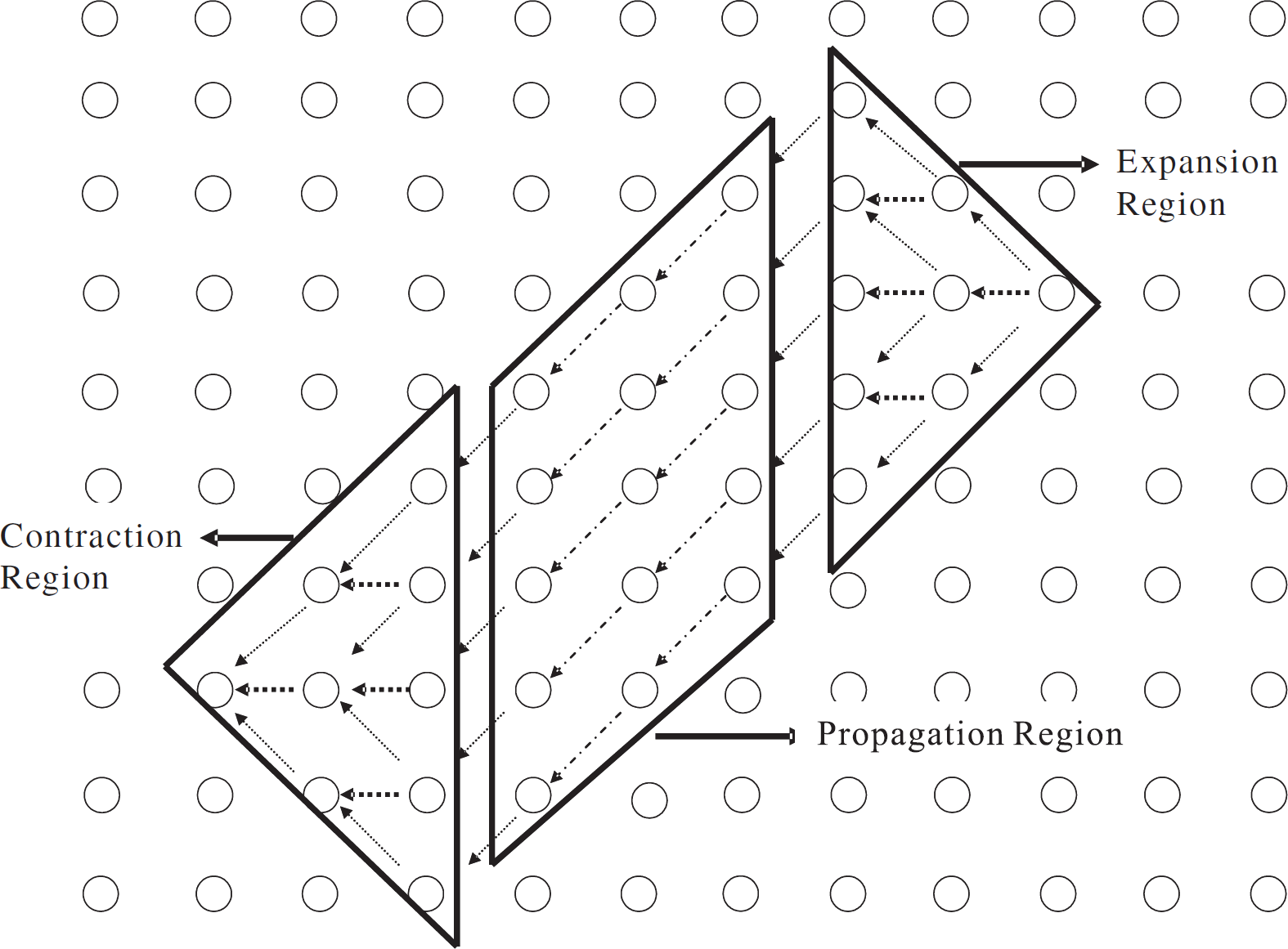
Three regions of contour.

The three regions of a contour are referred as the Expansion region, Propagation region, and the Contraction region and appear in every contour with a small variation between the rectangle shaped contour and the hexagon shaped contour.

Observation 6

In the expansion region, when each node is carrying an ideal number of messages, a node in a row of width w does not have sufficient number of messages for two nodes in the next row, i.e., row of width w + 2.

Proof

Since $\frac{N}{w}$ is the ideal number of messages that must be carried by each node in a row of width w, consider $\frac{N}{w} - \frac{N}{w + 2} = \frac{2 N}{w (w + 2)} \leq \frac{2 N}{w + 2}$ for all w ≥ 1. □

To illustrate the heuristic, consider Fig. 15. The nodes are in two successive rows of the expansion region in a contour. For convenience assume that the nodes are labeled as shown and that there are odd number of nodes in each row.

Figure 15.

Heuristic spreading in expansion.

Definition 4

Let w be the width of the contour in some row of the expansion region, and w + 2 be the width in the next row of the contour. Let w be odd. Let the nodes be labeled with, 1,2,3, …, ⌊w/2⌋ as shown in Fig. 15. Then, node i sends

\frac{i \times N}{w + 2} - \frac{(i - 1) \times N}{w}

messages to the node i on the next row. and

\frac{i \times N}{w} - \frac{i \times N}{w + 2}

messages to the node i + 1 in the next row.

For example in Fig. 15, when N = 70, w = 5, then, for the diagonal node node 1 sends 10 messages to node A, node 2 sends 6 messages to node B, etc. and for the node straight below, node 1 sends 4 messages to B, node 2 sends 8 messages to C, etc.

Using this heuristic, node A receives $\frac{N}{w + 2}$ messages from node 1; note that node A cannot receive messages from node 2. Node B receives $\frac{N}{w} - \frac{N}{w + 2}$ from node 1 and $\frac{2 N}{w + 2} - \frac{N}{w}$ messages from node 2 and, i.e., $\frac{N}{w + 2}$ messages. Similarly all the other nodes to the left of the middle node receive $\frac{N}{w + 2}$ messages. By symmetry, the nodes to the right of the middle node also use a similar spreading rule; except that the node that is the farthest from the middle node must be labeled 1. The middle node must send $\frac{N}{w + 2}$ messages to the middle node on the next row.

Definition 5

Let w be the width of the contour in some row of the propagation region, node i sends all its messages to the node i in the next row.

Definition 6

Let w be the width of the contour in some row of the contraction region, and w − 2 be the width in the next row of the contour. Let w be odd. Let the nodes be labeled with 1,2,3, …, [w/2] as shown in Fig. 16. Then, every node i sends

\frac{i \times N}{w} - \frac{(i - 1) \times N}{w - 2}

messages to the diagonal node on the next row and

\frac{(i - 1) \times N}{w - 2} - \frac{(i - 1) \times N}{w}

messages to the node straight below.

Figure 16.

Heuristic spreading in contraction region.

For example in Fig. 16, when N = 70, w = 7, then, for the diagonal node, node 1 sends 10 messages to node A, node 2 sends 6 messages to node B, and node 3 sends 2 messages to node C, etc. For the node straight below, node 2 sends 4 messages to node A, and node 3 sends 8 messages to node B, etc.

When the contour is a hexagon, there are special cases that must be considered. If w is the maximum width of the expansion region, the width of the propagation region is w + 1. The expansion heuristic (Definition 4) can be used by labeling the nodes as shown in Fig. 17. Similarly, when the maximum width of the contraction region is w − 1 and the contraction heuristic (Definition 6) can be used by labeling the nodes as shown in Fig. 18.

Figure 17.

Heuristic spreading in transition region.

Figure 18.

Heuristic spreading in transition region.

4. Simulation Results

Contour guided dissemination was validated via simulation and experiments. Section 4.1 presents the simulation tools used and Section 4.2 presents the results of the simulation. The number of messages handled in each node was used as the metric.

4.1. Simulation Approach and Tools

All the code developed for this investigation was developed in the NesC language [2] in the TinyOS environment [2]: targeting the MICA2 platform [1].

4.1.1. TinyOS

Four TinyOS components were developed to implement Contour Guided Dissemination. These components are shown in Fig. 19. DiscreteSensorM was used to generate periodic messages that represent values acquired from sensors. UpdateNeighborListM was used to periodically update the neighbors of each node. DiscreteSensorM sends events to HeuristicDS; this component implements the Heuristic spreading strategy. To implement weighted spreading or uniform spreading, the HeuristicDS components is replaced by a suitable component. TestHeuristicDS is a top-level component that is used to “wire” DiscreteSensorM, UpdateNeightborListM, and HeuristicDS into a Contour Guided Dissemination application.

Figure 19.

Contour guided dissemination application.

4.1.2. TOSSIM and PowerTOSSIM

The new components were simulated using TOSSIM [2]. The messages exchanged between nodes was viewed for debugging purposes using TinyViz [30], which is a visualization tool. TOSSIM also include a default propagation model for the wireless signals between nodes. Concern about the weakness of the propagation model in TOSSIM are well documented in literature [31]. Since the metric for this investigation was the number of messages handled, the known weaknesses were not a hinderance to this investigation.

To ensure that components are valid, they were compiled and executed in 4 MICA2 nodes. To ensure the consistency of the results, a plug-in extension to TOSSIM called PowerTOSSIM was used. PowerTOSSIM is based on an accurate model for energy consumption in the MICA2 platform [1]. When using PowerTOSSIM, it was ensured that each node of each step in the contour used approximately the same amount of energy. Since energy used linearly increases with the number of messages handled, this metric was useful to validate results. To ensure that the implementation of Contour Guided Dissemination was free from any other restrictions of the TOSSIM simulator, the components were validated via experiments in a 4 by 4 grid MICA2 nodes.

4.2. Simulation Results

The simulation results reported here were conducted on a grid of 9 × 9 motes. Every node can only communicate with 8 of its immediate neighbors (see Fig. 6). The maximum number of hops to the sink was 8. Two different source nodes were selected to obtain a hexagon contour and a rectangle contour. The selected source sent 100 messages to the sink.

4.2.1. Flooding with Duplicate Elimination

As a baseline measurement, the number of messages received by each node is measured when using flooding. In flooding, the source node sends each message to all its neighbors. Each node that receives a message forwards that message to all its neighbors. This process continues until the message is eventually received by the sink. To reduce the cost of flooding, duplicate elimination was used. Whenever a node received a message that it had already received before, the received message was discarded.

Flooding with Duplicate Elimination (FWDE) is an expensive method for communication. The number of messages received at each node after 30 sec and after 60 sec is shown in the top of Fig. 21. The bottom of Fig. 21 shows the messages after 90 seconds and 120 sec. As may be noticed, all the nodes receive the same number of messages and if 100 messages are sent, these 100 messages are received at all the nodes. Hence the energy consumption is really high in the network in order to forward all messages to the sink.

4.2.2. Gossiping with Duplicate Elimination

Gossiping with Duplicate Elimination (GWDE) is an alternative to flooding that can be used in dense systems. Instead of sending a message to all its neighbors, a node will randomly select one of its neighbors to send the message. Compared to flooding, this approach reduces the total number of messages that are sent. Despite the large number of messages that are sent, because of message loss and the random selection, the end-to-end delivery rate is neither consistent nor reliable. Figures 20 and 21 show the progression of messages after 30, 60, 90, and 120 sec.

Figure 20.

Flooding after 30 and 60 sec.

Figure 21.

Flooding after 90 and 120 sec.

4.2.3. Contour Guided Dissemination

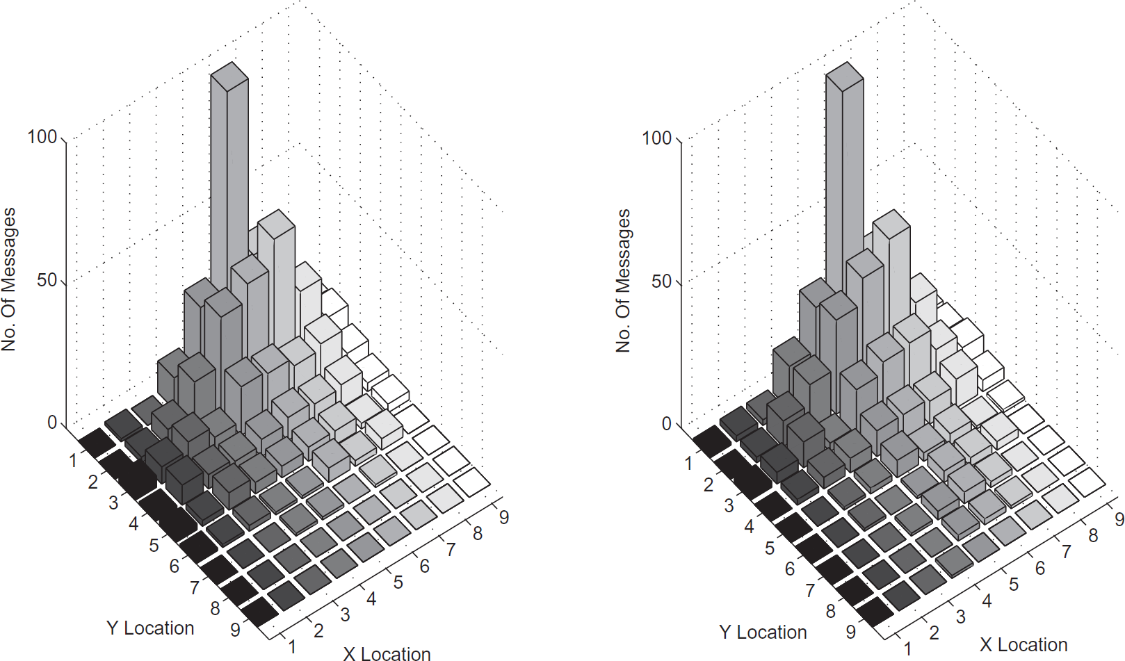
Figure 25 shows the number of messages in each node for the Contour Guided Dissemination method using uniform spreading. In this case, the contour of the shortest paths was a hexagon and a rectangle. Both these contours are in region 2 and it can be seen that the nodes along the diagonal carry more messages than other nodes in the contour. In other words, it is the heavily loaded boundary in the contour.

Figure 22.

Gossiping after 30 and 60 sec.

Figure 23.

Gossiping after 90 and 120 sec.

Figure 24.

Contour guided dissemination - uniform spreading in hexagon.

Figure 25.

Contour guided dissemination - uniform spreading in rectangle.

Figure 27 shows the number of messages in each node for the Contour Guided Dissemination method using weighted spreading. Because the region of the contour is known, the weighted parameters can be chosen so that more messages can be sent away from the diagonal line boundary. Therefore, the heavily loaded boundary condition in uniform spreading can be mitigated. The results are shown for both a hexagon contour and for a rectangle contour.

Figure 26.

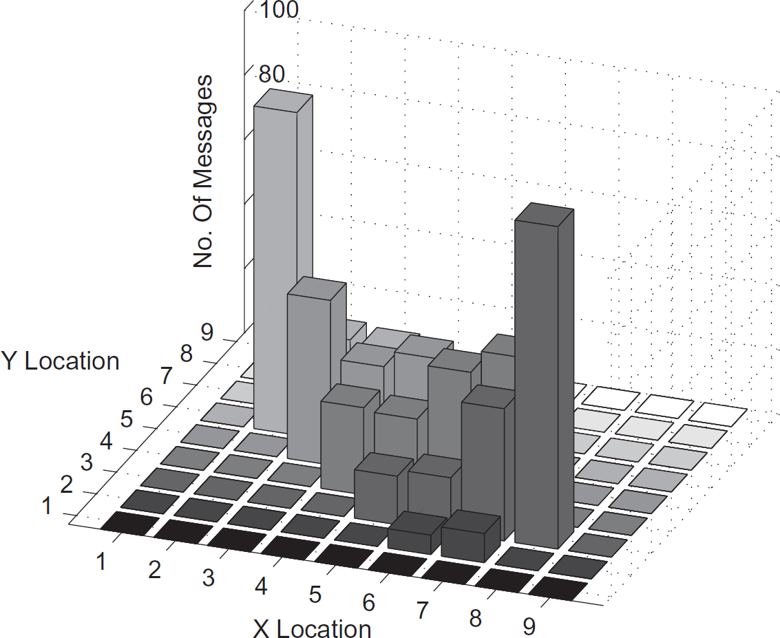
Contour guided dissemination - weighted spreading in hexagon.

Figure 27.

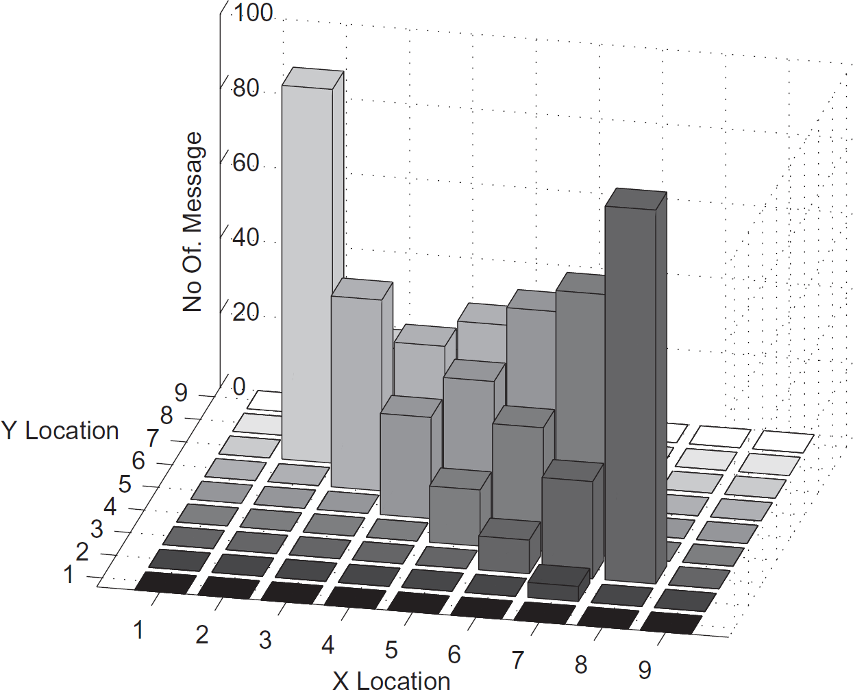
Contour guided dissemination - weighted spreading in rectangle.

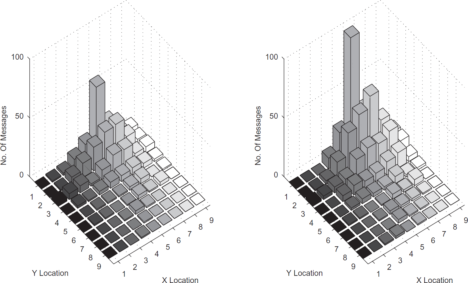
Figure 29 shows the number of messages in each node for the Contour Guided Dissemination method using the heuristic spreading method. It may be noticed that the number of messages in the contour is almost the same for all the nodes except the source and the sink.

Figure 28.

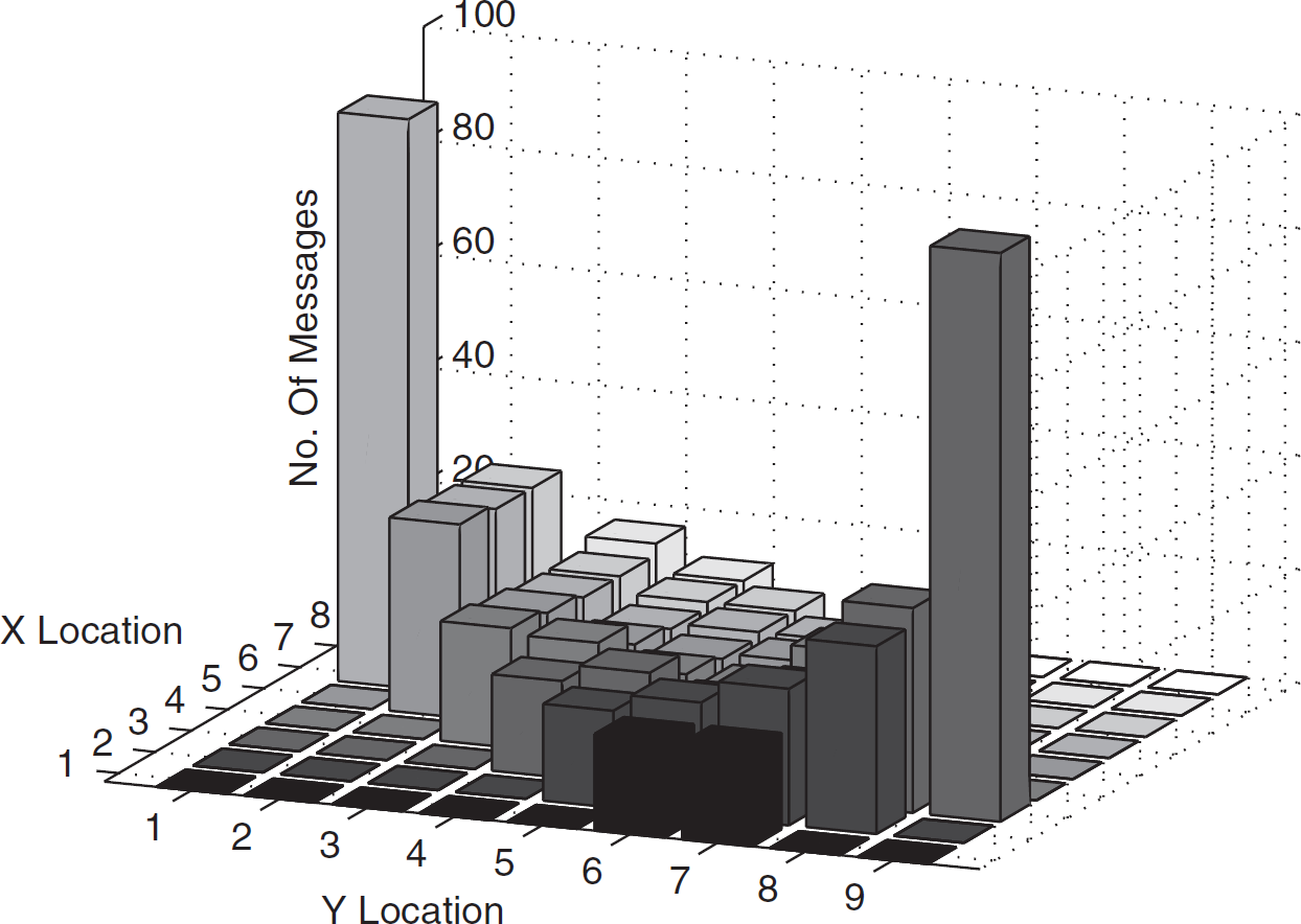
Contour guided dissemination - heuristic spreading in hexagon.

Figure 29.

Scalability comparison.

4.3. Summary and Discussion

FWDE is the easiest way to disseminate messages in the network, but this approach suffers from a tremendous amount of traffic because FWDE neglects the location of the sink and forwards the message to all its immediate neighbors. GWDE has less congestion in the network compared to FWDE. However, the end-to-end delivery rate is not high.

Uniform spreading in the shortest-path contour is the simplest form of Contour Guided Dissemination (CGD). Simulation results show that it performs better than simple methods that are based on a single path. Due to its simplicity, it has a heavily loaded boundary. The weighted spreading scheme mitigates this problem to an extent. Heuristic spreading performs well. This approach is a little complex in computation and the routing decision will depend on the source of the packet and the location of the sink and location of the node in the contour. To support the heuristic spreading scheme, the source must include the number of messages it is sending in the packet. This requirement is typically not unreasonable because in many engineering systems, diagnostic messages are sent in response to queries and based on the type of query, it will be possible to estimate the number of messages that must be sent.

Figure 29 shows a comparison between FWDE and Contour Guided Dissemination. It was noticed from the simulation that since the nodes using FWDE forward every message received, the maximum number of messages in the network grows at O(n²). On the other hand, it was observed in simulation that the number of messages in the network grows at O(n) when Contour Guided Dissemination was used. Figure 29 illustrates that Contour Guided Dissemination is more scalable than FWDE.

5. Conclusions

We presented a new approach, called Contour Guided Dissemination, for disseminating messages in networked embedded systems. This method exploits all the shortest paths available between a source and a sink.

The union of all the shortest paths between a source and a sink was defined to be a contour. The results in Section 3 show that when the value xy_diff is even, the shape of the contour is a rectangle and when xy_diff is odd, the contour is shaped like a hexagon. Because the theorems in Section 3 provide the locations of the corner nodes of the contour, these results are sufficient to allow each node to compute the contour in a distributed manner, and to identify its own position in the contour.

It was shown that when the messages are spread uniformly over the available paths, nodes on one edge of the contour handle more messages than the other nodes in the contour.

A heuristic spreading strategy was presented. It was shown through simulation results that the heuristic spreading strategy ensures that all the nodes in the same row on the contour handle approximately the same number of messages. Simulation results also show that the cost of communication in CGD compares very favorably with the cost of flooding. The cost of dissemination in this method increases linearly with the size of the grid.

Although the results were based on a regular topology, these results suggest new methods for dissemination in networks with general topologies. In such networks, some nodes must spread the messages, while other nodes must utilize one of the available paths without spreading the messages further. Identifying the structure of contours, expansion regions propagation regions, and contraction regions for networks with general topologies are interesting problems and the method presented here provides a systematic framework in which to carry out future investigations.

Footnotes

1

In addition to the sensors and actuators on the modules such an application would use additional devices such as cameras, RFID tags and scanners, weighing scales, etc., to inspect the entities that are being moved.

2

Such communication can be achieved by designing a suitable Medium Access Control protocol, using low-power steerable antennas, or multiple frequencies.

3

The assumption is that every monitoring station that wishes to receive monitoring messages from the networked embedded system will first register itself. This information is percolated through the network and every node is aware that there is a monitoring station that is interested in receiving messages.

4

Only the light colored part of the contours are shown.

References

Hill

Horton

Kling

Krishnamurthy

, “The platforms enabling wireless sensor networks in Communication of the ACM, vol. 47, no. 6, pp. 41–46, June 2004.

Hill

Szewczyk

Woo

Hollar

Culler

Pister

“System architecture directions for networked sensors,” in ACM Sigplan Notices, vol. 35, no. 11, pp. 93–104, 2000.

Iyengar

S.S.

Chakrabarty

H.C.

, “Distributed sensor networks for real-time systems with adaptive configuration,” Journal of the Franklin Institute, vol. 338, pp. 571–582, 2001.

Hayslip

Sastry

Gerhardt

, “Networked embedded automation,” in Assembly Automation, vol. 26, no. 3, 2006.

Chu

I-H.

Duan

Sastry

, “Contour guided dissemination for networked embedded systems,” in Innovative Real-time Applications of Distributed Sensor Networks, Baltimore, MD, October 2006.

Zhao

Krishnamurthy

Stankovic

, “Impact of radio irregularity on wireless sensor networks,” in MobiSys, pp. 125–138, 2004.

Lou

Zhang

, Dissemination Protocols for Large Sensor Networks, Kluwer Academic Publishers, 2004.

Bellman

R.E.

, Dynamic Programming, Princeton University Press, Princeton, N.J., 1957.

Dijkstra

, “A note on two problems in connexion with graphs,” Numerische Mathematik, vol. 1, pp. 269–271, 1959.

10.

Intanagonwiwat

Govindan

Estrin

Heidemann

Silva

, “Directed diffusion for wireless sensor networking,” in IEEE/ACM Transactions on Networking, vol. 11, no. 1, pp. 2–16, February, 2003.

11.

Kulik

Heinzelman

Balakrishnan

, “Negotiation-based protocols for disseminating information in wireless sensor networks,” in Wireless Networks vol. 8, pp. 169–185, 2002.

12.

Coulouris

Dollimore

Kindberg

, Distributed Systems Concepts and Design, Addison Wesley, Fourth edition, 2005.

13.

Akkaya

Younis

, “A survey on routing protocols for wireless sensor networks,” Ad Hoc Networks, vol. 3, pp. 325–349, 2005.

14.

Hedetnemi

Liestman

, “A survey of gossiping and broadcasting in communication networks,” Networks, vol. 18, no. 4, pp. 319–349, 1988.

15.

Coffin

Hook

D.V.

McGarry

Kolek

, “Declarative ad hoc sensor networking,” in SPIE Integrated Command Environments, 2000.

16.

Intanagonwiwat

Govindan

Estrin

, “Directed diffusion: a scalable and robust communication paradigm for sensor networks,” in Mobile Computing and Networking, pp. 56–67, 2000.

17.

Ganesan

Govindan

Shenker

Estrin

, “Highly resilient, energy efficient multipath routing in wireless sensor networks,” Mobile Computing and Communications Review, vol. 5, no. 4, pp. 11–25, 2002.

18.

Poor

R.D.

, “Gradient routing in ad hoc networks,” In http://www.media.mit.edu/pia/Research/ESP/texts/poorieeepaper.pdf.

19.

Zhang

, “Gradient broadcast: A robust, long-lived large sensor network,” in http://irl.cs.ucla.edu/papers/grab-tech-report.ps, 2001.

20.

Jain

Biswas

Nandiraju

Agrawal

D. P.

, “Energy aware routing for spatiotemporal queries in sensor networks,” IEEE, 2005.

21.

Heinzelman

Chandrakasan

Balakrishnan

, “Energy-efficient communication protocols for wireless microsensor networks,” in Hawaaian International Conference on Systems Science, 2000.

22.

Manjeshwar

Agrawal

D. P.

, “Apteen:a hybrid protocol for efficient routing and comprehensive information retrieval in wireless sensor networks,” in Proceedings of the International Parallel and Distributed Processing Symposium 2002, 2002.

23.

Heidemann

Estrin

, “Geography-informed energy conservation for ad hoc routing,” in MobiCom 2001, 2001.

24.

Govindan

Estrin

, “Geographical and energy aware routing: A recursive data dissemination protocol for wireless sensor networks,” Technical Report tr-01–0023, Dept. Of Computer Science, Univ. Of California, Los Angeles, 2001.

25.

Nath

Niculescu

, “Routing on a curve,” ACM Sigcomm Computer Communications Review, vol. 33, no. 1, pp. 155–160, 2003.

26.

Blum

B. M.

Abdelzaher

T.F.

Stankovic

J. A.

, “Rap: A real-time communication architecture for large-scale wireless sensor networks,” in Eighth IEEE Real-Time and Embedded Technology and Applications Symposium, 2002.

27.

Stankovic

J.A.

Abdelzaher

, “Speed a stateless protocol for real-time communication in sesnor networks,” in ICDCS, 2003.

28.

Heinzelman

Kulik

Balakrishnan

, “Adaptive protocols for information dissemination in wireless sensor networks,” in Proc. MOBICOM, Seattle, pp. 174–185, 1999.

29.

Agre

Clare

Sastry

A Taxonomy for Distributed Real-time Control Systems. Advances in Computers, Ed. Zelkowitz

, vol. 49, pp. 303–352, 1999.

30.

Levis

Lee

Welsh

Culler

“Tossim: Accurate and scalable simulation of entire tinyos applications,” Proceedings of the 1st International Conference on Embedded Networked Sensor Systems, in ACM SenSys, 2003.

31.

Titzer

Lee

Palsberg

“Avrora: Scalable sensor network simulation with precise timing,”

Proceedings of the 4th International Symposium on Information Processing in Sensor Networks, 2005.

Orientation	x _diff	y _diff	xy _diff
1	> 0	< 0	> 0
2	> 0	< 0	< 0
3	< 0	< 0	< 0
4	< 0	< 0	> 0
5	< 0	> 0	> 0
6	< 0	> 0	< 0
7	> 0	> 0	< 0
8	> 0	> 0	> 0

Orientation	x _diff	y _diff	xy _diff
1	> 0	< 0	> 0
2	> 0	< 0	< 0
3	< 0	< 0	< 0
4	< 0	< 0	> 0
5	< 0	> 0	> 0
6	< 0	> 0	< 0
7	> 0	> 0	< 0
8	> 0	> 0	> 0

Contour Guided Dissemination for Networked Embedded Systems

Abstract

Keywords

1. Introduction

1.1. Overview

2. Background

2.1. Dissemination Protocols

2.3. Example 1: Inspection Station

3.1. Contour of Shortest Paths

Definition 1

Definition 2

Observation 1

Proof

Lemma 1

Proof

Lemma 2

Proof

Lemma 3

Proof

Lemma 4

Proof

Theorem 1

Proof

Observation 2

Theorem 2

Proof

Observation 3

Observation 4

Proof

Observation 5

Definition 3

Observation 6

Proof

Definition 4

Definition 5

Definition 6

4.1. Simulation Approach and Tools

4.1.1. TinyOS

4.2. Simulation Results

4.2.1. Flooding with Duplicate Elimination

4.2.2. Gossiping with Duplicate Elimination

5. Conclusions

Footnotes

1

2

3

4

References

Orientation	x _diff	y _diff	xy _diff
1	> 0	< 0	> 0
2	> 0	< 0	< 0
3	< 0	< 0	< 0
4	< 0	< 0	> 0
5	< 0	> 0	> 0
6	< 0	> 0	< 0
7	> 0	> 0	< 0
8	> 0	> 0	> 0