Energy-Aware and Time-Critical Geo-Routing in Wireless Sensor Networks

Abstract

Volunteer forwarding, as an emerging routing idea for large scale, location-aware wireless sensor networks, has recently received significant attention. However, several critical research issues raised by volunteer forwarding, including communication collisions, communication voids, and time-critical routing, have not been well addressed by the existing work. In this paper, we propose a priority-based stateless geo-routing (PSGR) protocol that addresses these issues. Based on PSGR, sensor nodes are able to locally determine their priority to serve as the next relay node using dynamically estimated network density. This effectively suppresses potential communication collisions without prolonging routing delays. PSGR also overcomes the communication void problem using two alternative stateless schemes, rebroadcast and bypass. Meanwhile, PSGR supports routing of time-critical packets with different deadline requirements at no extra communication cost. Additionally, we analyze the energy consumption and the delivery rate of PSGR as functions of the transmission range. Finally, an extensive performance evaluation has been conducted to compare PSGR with competing protocols, including GeRaf, IGF, GPSR, flooding, and MSPEED. Simulation results show that PSGR exhibits superior performance in terms of energy consumption, routing latency, and delivery rate, and soundly outperforms all of the compared protocols.

1. Introduction

Geo-routing protocols have been widely adopted in the design of wireless sensor networks [24, 30, 38]. Most existing geo-routing protocols [1, 3, 6, 10, 20, 21] are stateful, i.e., make routing decisions based on cached geographical information of neighboring sensor nodes. However, possible node movements, node failures, and energy conservation techniques in sensor networks result in dynamic networks with frequent topology transients, and thus are not well-served by stateful packet routing algorithms. Recently, a number of studies (including our own work [35] and others [2, 8, 13, 40]) have proposed stateless geo-routing protocols for dynamic wireless sensor networks.

These stateless routing protocols leverage the key idea of volunteer forwarding in which the next relay node is not chosen by the packet holder (the node presently holding the packet), but instead by a set of volunteering neighbor nodes based on their geographical locations. Volunteer forwarding avoids the communication overhead of exchanging state information among sensor nodes, which in turn effectively reduces communication collisions and improves the energy efficiency of a routing protocol. Figure 1 illustrates the volunteer forwarding steps. Specifically, the packet holder broadcasts a forwarding probe message to its neighbors (Fig. 1a). Since georouting is expected to make geographical progress towards the destination, we define the nodes eligible for forwarding the packet (called potential forwarders) as those neighbors that are closer to the destination than the holder, and the area where PFs reside is called a forwarding region. Upon receiving the probe, the potential forwarders acknowledge according to some pre-designated priority (Fig. 1b). The first acknowledger receives the packet and becomes a new packet holder (Fig. 1c). This process is repeated until the delivery succeeds or fails. The probe message and acknowledgement message can be integrated with RTS/CTS messages from MAC layers for further reducing the communication overhead, as suggested by [2, 13].

Figure 1.

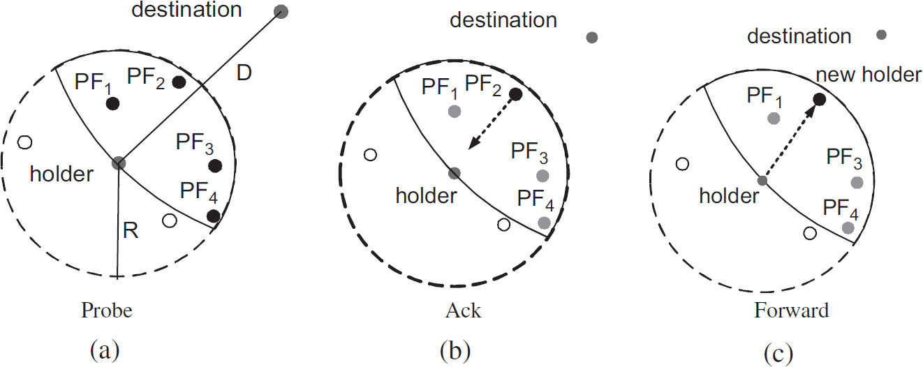
Volunteer forwarding.

There are two fundamental research issues involved in volunteer forwarding based geo-routing:

how to have potential forwarders autonomously determine their acknowledgement precedence without leading to excessive message collisions and routing delay;

how to detect and overcome the communication void problem (in case no potential forwarders exist).

Unfortunately, these two important issues have been only partially addressed in the existing studies [2, 8, 13, 35, 40], which either employ simple heuristics (so that the system performance is not optimized) or overlook the challenging communication void issue (see Section 2 for a detailed review). Another important issue, which, to our best knowledge, has not been addressed by any existing volunteer forwarding based protocol is time-critical routing. Our work indeed shows that volunteer forwarding is more suitable for supporting time-critical routing than stateful protocols. In stateful protocols, a packet holder chooses the next relay node only based on the communication delay that it experiences, without considering the delay that the neighbor node may experience when it transmits. As a result, the selected relay node may not be able to meet the routing deadline, and a costly recovery procedure has to be initiated.

In this paper, we present an in-depth study into the above research issues of volunteer forwarding. A novel protocol, called priority-based stateless geo-routing (PSGR), is proposed to achieve the following design objectives:

Stateless architecture. The physical constraints of a wireless sensor network (e.g., large scale, error-prone wireless communications, fragile sensor nodes, limited network resources) necessitate its protocols require minimal state requirements. By employing a volunteer forwarding scheme, PSGR relieves the sensor nodes from caching and maintaining network states required by stateful approaches [20, 28, 29].

Collision restraints. Communication collisions widely exist in wireless networks. They deteriorate network performance by increasing network traffic and prolonging communication delays. In PSGR, a priority-based autonomous acknowledgment mechanism consisting of

dynamic forwarding zone formation based on the sensor node density estimated on-the-fly, and

autonomous acknowledgement, is proposed to avoid the contention for the wireless broadcast channel among potential forwarders.

Resilience to communication void. Similarly to all geo-routing protocols, PSGR faces the communication void problem, in which a routing protocol fails to find a path to the destination, even when one actually exists. We overcome this problem by considering two complementary approaches, i.e., stateless rebroadcast and bypass, which favor different network scenarios.

Differentiated time-critical control. Multiple levels of communication criticalness are supported by PSGR. Unlike stateful time-critical routing protocols that may suffer from re-routing when packets are relayed to nodes incapable of meeting routing deadlines, the nature of PSGR (i.e., volunteer forwarding) allows unqualified sensor nodes to independently disqualify themselves from being the next relay node at no communication overhead.

Transmission range control. The transmission range of sensor nodes has significant impacts on energy consumption and delivery rate. We develop an analytical model with these two metrics as functions of the transmission range. The analysis provides insights on selecting radio transmission range and is important for planning and deployment of large-scale wireless sensor networks.

An extensive simulation is conducted to evaluate the performance of PSGR, against state-of-the-art geo-routing protocols including GeRaf [39, 40], IGF [2], GPSR [20], and flooding, and a time-critical routing protocol, i.e., MSPEED [7]. PSGR exhibits superior performances (in measured metrics of energy consumption, routing latency, and delivery rate) under various network conditions, and soundly outperforms all compared protocols.

The rest of the paper is outlined as follows. Section 2 presents the preliminaries and examines the related work, including stateful routing protocols and stateless volunteer forwarding based routing protocols. Section 3 presents the basic design of PSGR. Section 4 analyzes the appropriate transmission range for use in PSGR. Section 5 reports our performance evaluation and simulation results. Finally, Section 6 concludes the paper with a summary and discussion of future work.

2. Preliminaries and Related Work

Here we present the preliminaries needed for this work and examine some closely related research.

2.1. Background

We assume a wireless sensor network consisting of a large number of sensor nodes deployed within a vast two-dimensional field. The network is location-aware, i.e., each sensor node is able to obtain its location information through an equipped GPS component [27] or some localization technique [32]. Moreover, sensor nodes can adjust their transmission range R between (0, R_max] for each transmission, where R_max is the maximum transmission range. Energy consumption for transmitting one bit with transmission range R is captured as Etx(R) = E_elec + E_ampR^α, where E_elec and E_amp denote the energy consumed by the radio transmitter and the transmission amplifier, respectively; α, called the path loss factor, usually satisfies 2 ≤ α ≤4. It takes Erx(R) = E_elec to receive one bit.

The sensor network topology may dynamically change during operation. The dynamics of a sensor network may be introduced by

node mobility (sensor nodes may be mobile);

energy conservation (sensor nodes may periodically switch to sleep mode [5, 31, 34]);

unreliable links and node failures.

Without loss of generality, we assume each sensor node in the network may move without exceeding a maximum speed of V_max (the sensor nodes are stationary when V_max = 0). Mobile sensor networks have received increasing research attention [15, 16, 35]. The mobility of sensor nodes triggers a wide range of new applications. For example, by scattering a collection of floating sensor nodes into a pond, the condition of the pond can be monitored more effectively than by a set of stationary nodes. This paper focuses on the routing of data packets from a source node to a geographical location rather than to a specific sensor node.

This assumption is justified by many sensor network-supported applications, which are interested in physical phenomena associated with a geographical location or region, but are not aware of the geographical distribution of the sensor nodes [36].

The routing process terminates when

the data packet reaches a sensor node located within some distance threshold from the destination (e.g., within the transmission range R), or

a sensor node believes that the destination is not reachable, or cannot be reached before a specified time, and drops the packet.

The first condition designates a successful delivery while the second condition represents a delivery failure. The exact criteria for a node to decide when to drop a packet depends on the strategies for overcoming the communication void problem and on the routing deadline requirements, which are further discussed in Section 3.2 and Section 3.3, respectively.

2.2. Related Work

Our work has been inspired by a number of research efforts. In this section, we examine the work most closely related to our proposal, in particular the work that we study in our performance evaluation (i.e., GPSR, IGF, GeRaf, and MSPEED).

Many routing algorithms proposed for ad hoc networks, e.g., AODV [28], DSR [18] and DSDV [29], are stateful. Each node has to maintain up-to-date end-to-end routing information (i.e., link states) for a number of destination nodes. To accommodate the dynamic changes of network topology, nodes have to periodically exchange messages to update the cached link states; this intensifies the network traffic and consumes precious network resources.

GPSR [20] is a representative stateful geo-routing protocol in which a packet holder makes routing decisions based on the locations of neighbor nodes. In GPSR, nodes cache locations of their neighbor nodes. The cached information is periodically refreshed via beacon messages. If a node does not hear from a neighbor within a certain period of time, it assumes the neighbor is not available and thus removes the corresponding information from its cache. GPSR works in two modes: greedy forwarding and perimeter forwarding. In greedy forwarding, a packet holder, based on the cached locations of neighbor nodes, chooses the neighbor closest to the destination as the next relay node. GPSR switches to a perimeter forwarding mode when reaching a void region. Perimeter forwarding employs a right-hand rule to route the packet around the void region, then greedy forwarding resumes when the packet reaches a node closer to the destination than the node at which the packet enters the perimeter mode. Due to the dynamic network topology, it is possible that the cached information is obsolete and that a holder chooses a relay node that is not closest to the destination or even not inside the holder's transmission range. GPSR relies on the MAC layer to detect the latter case. Once a broken link is detected, the holder updates its cache, selects the second closest neighbor to the destination from its cache, and resends the packet. This procedure could be repeated multiple times before the packet is successfully forwarded. Thus, GPRS is inefficient for dynamic sensor networks.

IGF [2] is a stateless algorithm based on volunteer forwarding. In IGF, a forwarding region is defined as a 60-degree fan-shaped area that faces toward the destination. IGF assigns acknowledgement precedence to each location point in the forwarding region based on its distance to the destination plus a random delay. IGF intends to have PFs closer to the destination acknowledge earlier, but fails to minimize the routing delay because there is a potentially infinite number of location points in the forwarding region. Consequently, a packet holder may have to wait for a long time before hearing an acknowledgement back. IGF proposes forwarding region shift to address the communication void problem. A packet holder that does not receive acknowledgements can request a shift in a forwarding region by retransmitting the probe message to search for an available PF in the new region. The shift stops when a PF is found or when no PF can be found in the entire transmission area of the holder. The latter case represents a packet delivery failure.

GeRaf [39, 40] is another stateless geo-routing protocol based on volunteer forwarding. The forwarding region in GeRaf is the intersection of the circle centered at the packet holder with transmission range as its radius and the circle centered at the destination with the distance between the packet holder and the destination as its radius. GeRaf has a larger forwarding region than IGF and thus has a better chance of locating a PF. Similar to our proposal, GeRaf divides the forwarding region into a number of sub-regions (we call them forwarding zones (FZ) in PSGR), each of which qualifies a distance to the destination. To reduce the routing latency, PFs located in the same FZ are assigned the same priority and thus will compete with each other.

GeRaf does not try to minimize acknowledgement collisions, but rather provides a resolution for them. Thus, it does not determine appropriate forwarding zones and acknowledgement delays as PSGR does. In the event of acknowledgement collisions, the holder broadcasts a collision message. Upon receiving this message, each colliding PF decides (with probability 0.5) whether or not to resend the acknowledgment. This resolution algorithm repeats until the collision is resolved or a maximum number of collisions is reached, in which case an abort message is broadcast by the holder. If no acknowledgment from a forwarding zone is received after a pre-designated period of time, the holder issues a continue message which triggers all PFs in the next forwarding zone to send the acknowledgement messages. The above procedure is repeated until either the holder finds a relay node or it searches the entire forwarding region without finding any PF. For the latter case (i.e., communication void problem), GeRaf leverages the dynamics of network topology and suggests that the holder wait for a period of time then search its forwarding region again. However, no details are provided in [39, 40].

BLR [13] and CBF [8], which employ similar ideas to IGF and GeRaf, are not examined in our performance evaluation due to the lack of design details and system settings. While BLR uses a forwarding region similar to IGF's and CBF uses the same forwarding region as GeRaf, both BLR and CBF assign acknowledgement precedence in the same way as IGF. In BLR, a Max_delay parameter, indicating the maximum delay a packet can perceive per hop, is used to calculate the acknowledgement delay for each node. However, the choice of Max_delay, which clearly has an impact on communication collisions, forwarding latency, and energy consumption, is not explored in the work. BLR handles the communication void problem by relaying a packet to the node that has the smallest angle between itself, the previous holder and the destination. Other issues, such as reusing the forwarding path for continuous routing and aggregation of the paths, are touched upon without providing details. CBF does not address the communication void problem.

To our best knowledge, no existing volunteer forwarding based schemes support time-critical routing, though several stateful routing protocols have been proposed for time-critical routing in ad hoc and sensor networks. In [19, 25, 33], routing decisions adapt to the network traffic by MAC layers, but does not aim at end-to-end time-critical communications. SPEED [11, 12] proposes a cross-layer (i.e., MAC and network layers) method to deal with the above issue. SPEED does not differentiate the routing deadlines for different packets. MSPEED, proposed in [7], overcomes this deficiency of SPEED. In MSPEED, each node maintains a delay estimation and a metric of SPEED to each neighbor node. The SPEED metric is the ratio of the geographical distance to the transmission delay between the node and the neighbor node. The time constraint of a packet is defined by a SetSPEED, which is the ratio of the geographical distance between the source and the destination to the routing deadline. The packet holder forwards the packet to a neighbor node if the SPEED to this neighbor node is higher than the SetSPEED of the packet. However, in addition to the inherent deficiency of stateful routing protocols, MSPEED has another major drawback. In the selection of relay nodes, the packet holder only takes into consideration its SPEED to the neighbor node, but not the ability of the selected relay node to meet the routing deadline. Thus, when an unqualified neighbor node is chosen as the relay node, a back-pressure re-routing has to take place, in which the packet is routed back to the previous packet holder(s) to look for other neighbor nodes as the relay node. This re-routing leads to increased communication costs and communication delays. The nature of volunteer forwarding overcomes this problem efficiently. In PSGR, the potential forwarders estimate their own communication delay to determine whether they are qualified to relay the packet. As a result, each relay node is ensured able to meet the routing deadline.

3. Design of PSGR

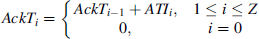
Our design of PSGR aims to provide robust and efficient routing protocols for wireless sensor networks. The PSGR framework is shown in Fig. 2. Volunteer forwarding, in which relay nodes are selected without knowledge about the network states, is the core of PSGR. A prioritized acknowledgment scheme, empowered by on-the-fly estimation of node density, dynamic formation of forwarding zones, and minimized acknowledgment delay for each forwarding zone, is able to suppress competing acknowledgement message collisions. This is discussed in Section 3.1. Stateless rebroadcast and bypass, presented in Section 3.2, are two alternative strategies for resolving the communication void problem. Time-critical control is crafted to support differentiated routing deadlines; this is discussed in Section 3.3. The last component, transmission range control, will be presented in Section 4.

Figure 2.

PSGR framework.

3.1. Prioritized Acknowledgement

The basic idea of prioritized acknowledgement is to assign acknowledgement precedences to all the PFs such that the PFs can respond to a forwarding probe without competing with each other. An intuitive scheme is to assign a unique acknowledgement precedence value (denoted as AckP) to every location point in the forwarding region in accordance with a total order relationship among all the location points. This total order relationship can be governed based on various heuristics such as the distance to the destination. Thus, a PF can autonomously decide its own AckP after receiving a probe. This is the approach IGF, BLR, and CBF adopt to aviod acknowledgement collisions. However, this naive scheme faces a challenge in terms of the acknowledgement delay (i.e., waiting time), since many location points are not occupied by any PF. Consequently, a packet holder may have to wait for a long time before hearing an acknowledgement. In PSGR, we assign an AckP to a forwarding zone instead of to a location point. A forwarding zone is dynamically formed such that acknowledgement collisions rarely happen and acknowledgement delays are minimized. Furthermore, PFs (whether within the same or different zones) determine their acknowledgement delay autonomously without any intervention from the packet holder.

In the following, we discuss in detail three important aspects of zone formation in PSGR: scope, size and acknowledgment delay.

3.1.1. Zone Scope

The scope of a forwarding zone refers to the covered area of the zone. The forwarding region can be divided into forwarding zones based on various heuristics that provide a total order among the zones. We explore two heuristics for optimizing the energy consumption and routing latency, respectively.

The first heuristic, called distance to the destination (DTD), aims at maximizing the spatial forwarding progress at each hop. The forwarding region (denoted as FR) is partitioned into Z forwarding zones FZ_i (1 ≤ i ≤ Z). Let D denote the distance between the holder and the destination. An FZ_i in PSGR is represented with a pair of distances to the destination, i.e., 〈d_i-1, d_i〉, where d₀ is set to D - R, and d_i (1 ≤ i ≤ Z) is selected such that the area of each FZ_i equals the expected zone size (see next subsection). Thus, FZ_i = {p|d_i-1 ≤ |p - p_D| ≤ d_i Λ |p - p_S| ≤ R} and $FR={\cup }_{1\le i\le {\text{ZFZ}}_{\mathrm{i}}}$ , where R is the radio transmission range, and p_S and p_D are the positions of the holder and destination, respectively. Figure 3a shows that forwarding zones created based on DTD; they are numbered based on their closeness to the destination. For all PFs residing in FZ_i, the AckP equals i.

Figure 3.

Forwarding zones.

The second heuristic, called modified DTD (M_DTD), first splits the forwarding region into sectors, such that ∀PF_a, PF_b ∊ S_i: |PF_a − PF_bR, where S_i denotes sector i and |PF_a − PF_b| represents the geographical distance between PF_a and PF_b. In this case, a PF can hear all the communications originated from the sector in which it resides. For example, as shown in Fig. 3b, an FR is divided into three sectors, Sector 1, with vertices V₁, V₂, and the holder, is surrounded by three arcs. An arc between any two vertices is a partial circumference of the circle centered at the remaining vertex with the transmission radius R. Sectors 2 and 3 are on either side of sector 1. Within each sector, M_DTD further forms FZs by applying the DTD heuristic, as marked by the dotted lines in Fig. 3b. Hence, two PFs located in adjacent FZs that are in the same sector can hear each other. This has a positive effect on reducing the acknowledgement delay, which will be explained shortly in Section 3.1.3. The AckP of a forwarding zone is assigned based on a combination of its sector number and its distance to the destination.

3.1.2. Zone Size

The size of an FZ determines the number of zones within the FR. When the FZ size is set to the size of the FR, the holder faces the issue of duplicated acknowledgements and collisions. On the other hand, when the FZ is reduced to a location point, the holder faces the issue of long acknowledgement delay. PSGR avoids these two extremes by dynamically setting the forwarding zone to an average area in which only a single PF resides. This design goal, achieved by taking dynamically estimated node density into account, contributes significantly to the novelty and excellent performance of PSGR.

Let A(d, r₁, r₂) denote the size of an area intersected by two circles with radii being r₁ and r₂, respectively, and the distance between their centers being d. Let D be the distance between the holder and the destination. The area of the holder's forwarding region can be represented by A(D, D, R). Suppose the estimated density, ρ, of sensor nodes is (see the next paragraph for the estimation method); the FZ size is obtained as 1/ρ. Thus, the total number of FZs can be obtained as Z = ⌈A(D, D, R) · ρ⌉. The exact scope of an FZ and its corresponding acknowledgement precedence value (i.e., AckP) can then be obtained as described in the previous subsection.

To estimate the density of neighbor sensor nodes, ρ, the holder records the number of unique nodes residing in its radio transmission area (i.e., with an area of πR²) within a certain time window. This is obtained from the messages the holder overhears/hears. We set the time window as the average time a neighbor node remains active inside the coverage area of the given sensor node. We first consider a mobile network with moving sensor nodes. Let crossing rate, τ, denote the number of nodes crossing a given region per second. According to [4], $\tau =\frac{\rho V_{max}C}{\pi }$ , where V_max is the maximum moving speed of sensor nodes, and C is the perimeter of the given region. The perimeter of a sensor node's coverage area is C = 2πR, and thus the crossing rate is τ = 2ρV_maxR. Since the average number of nodes in the coverage area of the given sensor node is ρπR², we obtain the average time that a node remains in the radio coverage region of a sensor node as $\frac{\rho \pi R^2}{\tau }=\frac{\pi R}{2V_{max}}$ . We next consider a stationary network in which some or all sensor nodes are periodically switched to the sleep mode for a period of time ranging in [0, t_max] seconds. Thus, the average time a node is active in an FR is t_max/2. However, this estimate method works only when the network traffic is heavy enough. When few communications happen inside the network, the sensor node may have an estimate lower than the actual density of its neighbor nodes. Therefore, we set a lower bound for the node density, ρ _d , which is obtained by assuming a uniform node distribution in the operational area. We remark that this density estimation does not conflict with the key idea of stateless volunteer forwarding, since no state information of neighboring nodes, except for a count of messages heard, needs to be maintained and updated.

3.1.3. Acknowledgment Delay

We use an acknowledgement timer to specify the acknowledgment delay (denoted as AckT) that a PF needs to wait for before it responds to the holder. Let ATI_i denote the acknowledgement timer interval associated with FZ_i. For a PF located in FZ_i, AckT_i can be obtained as follows:

$$Ack{T}_i=\{\begin{array}{cc}Ack{T}_{i-1}+AT{I}_i,& 1\le i\le Z\\ 0,& i=0\end{array}$$

(1)

To optimize acknowledgement delay, ATI_i (1 < i ≤ Z) should be as small as possible, yet it should be long enough that a PF can hear the acknowledgement from high-priority PFs or the packet from the holder before its timer expires. In other words, ATI_i should be long enough to accommodate the elapsed time from the instance when a sensor node initiates a message to its farthest neighbor node to the instance when the neighbor node receives it. This delay can be estimated as propagation delay + network delay, which will be further discussed in Section 3.3. Regarding the ATI_i setting for FZ_i, there are two cases:

If all the PFs inside FZ_i can hear possible acknowledgements sent from FZ_i−1 (e.g., with M_DTD shown in Fig. 3b), the ATI_i for each FZ_i is set as one time of delay.

Otherwise, ATI_i is set to twice the delay: the extra delay is for the PFs inside FZ_i to hear whether the packet has been forwarded from the packet holder.

PSGR attempts to form zones that each contains only one PF in order to avoid acknowledgement collisions. However, with a possibly non-uniform node distribution and an imperfect estimate of node density, there is no guarantee that there is only one PF in each FZ. The solution to this problem, widely adopted by many communication protocols in sensor networks [2, 17, 20, 34], is to add a small jitter (i.e., a random delay drawn from a range) to each AckT_i. This method is simple yet effective. To maintain the total order relationship in PFs, in calculation of AckT_i, a maximum jitter (i.e., the longest jitter allowed) is added to the right hand side of Equation (1).

3.2. Communication Void Problem

In a dynamic network topology, the void regions may be temporary. Additionally, a void region may be created due to a short transmission range used by a packet holder. In PSGR, a void region is detected if a packet holder does not receive any acknowledgment after all the forwarding zones time out. In this case, the packet holder is called a stuck node. We propose complementary stateless rebroadcast and stateless bypass strategies to go across or to go around the void region, respectively, without requiring a priori knowledge about network and neighbor states.

3.2.1. Stateless Rebroadcast

The rebroadcast strategy is based on the belief that a PF may exist near (or actually sleep within) the void forwarding region of the packet holder.

Our rebroadcast algorithm for the void communication problem runs as follows. Once a void region is identified, the holder resets a rebroadcast timer in hope that some sensor node(s) will become available in its forwarding region. When the timer expires, the forwarding request is rebroadcast with the maximum transmission range R_max in order to increase the probability of hitting a PF in this extended forwarding region. If the holder receives an acknowledgement, it sends out the data packet and returns to the regular forwarding process. Otherwise, the rebroadcast repeats until a sensor node enters into the forwarding region or a present number of rebroadcasts is reached. ¹

In PSGR, the rebroadcast timer is determined by considering the average sleep period and the mobility of the sensor nodes. We first consider mobile networks with moving sensor nodes. As mentioned in Section 3.1.2, τ denotes the crossing rate and equals $\frac{\rho V_{max}C}{\pi }$ where ρ is estimated as described previously. Given the transmission range R, and the distance D between the holder and the destination, the perimeter of the forwarding region is $C=2R{cos}^{-1}(\frac{R}{2D})+2D{cos}^{-1}(\frac{2D^2-R^2}{2D^2})$ . The average time for a sensor node to move into a given FR is given by 1/τ:

$$\frac{1}{\tau }=\frac{\pi }{\rho V_{max}(2R{cos}^{-1}(\frac{R}{2D})+2D{cos}^{-1}(\frac{2D^2-R^2}{2D^2}))}$$

Given a stationary network with sensor nodes periodically switching to sleep mode, the average time that a node appears in a given FR is t_max/2, where t_max is the maximum sleep period of sensor nodes. Thus, we set the rebroadcast timer to be MIN $(\frac{1}{\tau },\frac{t_{max}}{2})$ . Prolonging the timer increases the chance of a node appearing in the forwarding region, reduces the number of rebroadcasts needed, and improves the delivery rate, at the cost of forwarding latency.

3.2.2. Stateless Bypass

The rebroadcast strategy is not expected to perform well when the packet holder encounters a permanent void region or when PFs do not quickly appear in the forwarding region. Thus, an alternative bypass strategy is still necessary. PSGR's bypass algorithm is based on the well-known sweeping rule ² , which we tailored for dynamic wireless sensor networks. This sweeping rule exploits the properties of cyclic traversal to route around the voids, as it traverses the interior (exterior) of a closed polygonal region in the clockwise (counterclockwise) order.

During the regular forwarding process of PSGR, the sensor nodes located in the packet holder's transmission range, but not within the forwarding region (thus called potential bypassing nodes (PBs)) anticipate the potential bypass events by setting their bypassing acknowledgement precedences and timers when receiving a forwarding request message from the holder. The AckTs for PBs are longer than the AckTs of all the PFs, so PBs do not compete with PFs. A PB stops its timer if it overhears a message from the holder, PFs or any other PBs before the timer expires. Otherwise, when the timer expires it acknowledges the holder (i.e., the stuck node) that it will serve as a bypassing node. The routing process then switches from forwarding to bypassing mode. Once a PB becomes a bypassing node, it roadcasts a bypassing probe message. For the subsequent selection of bypassing nodes, all the neighboring nodes located within the transmission range are PBs. According to the bypassing priority and timer (determined by the sweeping rule), the PB who first acknowledges the bypassing node will take the data packet and continue the bypass process. If this PB is located closer to the destination than the stuck node, the forwarding mode is resumed. Moreover, in order to prevent loops (since the sensor nodes have no knowledge of network topology or network underlying graph), bypassing nodes keep track of the packets they have previously received for bypass and disqualify themselves as PBs when they hear the same bypassing probe again. In the rare occasion where the routing cannot be quickly brought back to forwarding mode, a count of bypass hops is used to terminate the packet delivery.

Following the sweeping rule, a bypass routing typically circumvents closely along the border of a void region. This strategy has been shown to work well in previous studies [6, 20, 23]. However, we observe that this approach may incur high routing cost and/or routing failure when a bypassing route makes a turn. Intuitively, a bypassing route makes a turn when no PBs are available for bypassing on one side of the void region. We define that a bypassing route makes a turn when the segment connecting the current and next PB nodes intersects with the line connecting the stuck node and the destination. In the existing algorithms, once a sweeping direction is determined (clockwise or counter-clockwise), this direction is fixed during the entire bypass, which very likely results in a much longer trajectory or even a delivery failure when the bypassing routes make a turn (as shown by Curve (2) and (4) in Fig. 4a).

Figure 4.

Bypass communication void region.

In PSGR, we allow the bypassing node to adjust the sweeping direction. More specifically, if the first bypassing node is found without sweeping for over 180°, the subsequent sweeping remains in the same direction, otherwise the sweeping direction is switched to the opposite one. This direction remains unchanged, except when the bypassing route makes a turn, in which case the subsequent sweeps switch to the opposite direction. In Fig. 4a, by performing the initial sweep in the clockwise direction, the first bypassing node is found at the East side of the separating line. Since this sweep does not go over 180°, all subsequent sweeps at the same side will be performed in the clockwise direction. Curve (1) shows a scenario where bypass circumvents along the East border of the pond and returns back to forwarding mode. However, assuming the absence of node X, Curve (2) shows the bypass routing enters into the West side. Based on our algorithm, the subsequent sweeps at the West side will go in the counter-clockwise direction. This direction switch is critical, as shown by Curve (3), because it leads to a routing trajectory that circumvents the void region from the West side more efficiently as comparing against bypassing with a fixed sweeping direction (as shown by Curve (4)).

To adapt to the frequently changing network topology, the bypassing algorithm described above actually makes use of the same idea of volunteer forwarding. Acknowledgment priority and timer are employed again to control the waiting time and to suppress the duplicate messages from PBs. The main difference is that, instead of using heuristics such as the distance to the destination in DTD scheme, the bypassing zones are formed in accordance with the sweeping rule. As illustrated in Fig. 4b, fan-shaped bypassing zones are obtained such that only one node is expected to be in a zone.

3.3. Time-Critical Routing

Sensor networks are used to monitor the physical phenomena that change over time. In many sensor network applications the data, including sensor readings, application commands and network control messages, only remain valid or useful within a certain period of time and become invalid or useless after that. Thus, a packet p_i has to be routed from a source to a destination within a period of time called the routing deadline (denoted as RD (p_i)). The routing deadline defines the upper bound of the routing delay that can be tolerated.

The routing deadlines for different packets could be different based on the packet contents and/or application requirements. For instance, a packet carrying an emergency alert is usually associated with a short routing deadline, so that the destination can make prompt reactions upon receiving the alert message. On the other hand, a packet containing a periodic report about the environmental temperature can tolerate a longer routing delay. We argue that, in making a routing decision, the routing deadline of a packet has two uses:

implying the priority of the packet being relayed by a packet holder, and

estimating a potential forwarder's ability to meet the routing deadline.

Existing time-critical routing protocols [7, 11] usually consider the first implication, but fail to take advantage of the second use of the routing deadline when choosing the relay nodes. These protocols choose a relay node based on the estimated delays between the packet holder and all its neighbor nodes. Since the delay estimates are maintained by the packet holder, the selected relay node may not be able to meet the requirements of the packet. In this section, we show that the volunteer forwarding scheme naturally overcomes the above problem and thus is more suitable for supporting time-critical routing than the stateful routing protocols.

A packet p_i to be routed is defined by a source node as < p_i, StaT(p_i), RD(p_i) >, where StaT (p_i) is the time at which the source node sends out p_i and RD (p_i) is the routing deadline for packet p_i. Thus, StaT (p_i) + RD (p_i) defines the latest time when p_i can arrive at the destination. Routing of p_i is considered as a failure if any relay node or the destination receives p_i after Stat(p_i) + RD(p_i). In addition to the information described in Section 3.1, the probe message from a packet holder also contains StaT(p_i) and RD(p_i). Each PF, upon receiving the probe, determines whether the routing can meet the deadline if it acts as the next relay node. If the decision is negative, the PF drops the probe message and does not compete with other PFs to acknowledge the packet holder. Otherwise, the PF sets its acknowledgment timer as discussed in Section 3.1.3. To check its qualification for being the relay node, a potential forwarder PF_k estimates the communication delay of sending packet p_i (denoted as delay_k (p_i)) as consisting of the propagation delay, the network delay and the scheduling delay:

Propagation delay is used for transmitting a packet a physical distance between two nodes. The propagation delay can be calculated a priori based on the network bandwidth.

Network delay is the period of time that a node waits for the broadcast channel to be available for transmission. Given the wireless broadcast medium in sensor networks, the network delay of a sensor node can be learned from the communication around this node [12].

Scheduling delay of p_i is caused by the packets that are scheduled to be relayed by node PF_k before p_i.

The scheduling delay is affected by the scheduling policies. As packets may have different routing deadlines, a simple First-In-First-Out (FIFO) scheduling policy seems inappropriate. In the following, we examine two other scheduling policies ³ for assigning transmission priority to p_i (denoted by txp(p_i)).

Earliest routing deadline first (ERDF): The transmission priority of a packet is purely determined by the routing deadline, i.e.,

$$txp(p_i)<txp(p_j),\text{iff\hspace{0.5em}}StaT(p_i)+RD(p_i)<StaT(p_j)+RD(p_j)$$

If StaT(p_i) + RD(p_i) = StaT(p_j) + RD(p_j), their priorities are randomly determined.

Least slack first (LSF): The transmission priority of a packet is determined by the slack time, which is an estimate of how long a packet can be delayed while still meeting its deadline.

$$\begin{array}{rl}& txp(p_i)<txp(p_j),\\ & \text{iff\hspace{0.5em}}StaT(p_i)+RD(p_i)-EstRT(p_i)<StaT(p_j)+RD(p_j)-EstRT(p_j)\end{array}$$

where EstRT (p_i) is the estimate of the remaining time needed for routing packet p_i. EstRT (p_i) can be derived from the lower bound of the number of hops for routing from PF_k to the destination (denoted as h_PFk and will be discussed shortly in Section 4), and the communication delay experienced previously during routing [11]. If StaT(p_i) + RD(p_i) - EstRT(p_i) = StaT(p_j) + RD(p_j) - EstRT(p_j), their priorities are randomly determined.

With estimated delay_k (p_i), PF_k determines whether it can meet RD(p_i) by examining

$$\frac{RD(p_i)-StaT(p_i)-T}{dela{y}_k(p_i)}<h_{P{F}_k}$$

where T is the current time, and $\frac{RD(p_i)-StaT(p_i)-T}{dela{y}_k(p_i)}$ is the estimated remaining number of hops needed for reaching the destination node. If this inequality holds, routing via PF_k is very likely to miss the routing deadline, as h_PFk serves as the lower bound of the remaining number of hops needed for routing. More specifically, PF_k gives up competing with other PFs to be the next relay node when one or more following conditions are satisfied:

its outgoing packet queue is full;

PF_k cannot meet RD(p_i) (i.e., the above inequality holds);

after scheduling p_i, the routing deadlines of other packets, which were already scheduled by PF_k are not satisfied anymore.

Examining the above inequality is a local operation performed by PF_k without any knowledge about other sensor nodes. Thus, the decision may not be optimal. Nevertheless, a bad local decision can be remedied by the subsequent relay nodes along the routing paths, as our scheduling polices take routing timeliness into consideration when assigning transmission priority. Therefore, the packets with tighter timeliness requirements obtain higher transmission priority. When no PF inside the holder's forwarding zone is able to satisfy the timeliness requirement of p_i, the packet holder hears nothing from its forwarding zone. In this case, the holder handles the situation as it encounters a void region using either rebroadcast scheme or bypassing scheme, while those PFs or PBs that cannot meet the routing deadline for packet p_i again are not considered.

Figure 5 summarizes the mechanisms discussed above for achieving the collision control and time-critical control. The dotted line specifies that the routing deadlines of packets have an impact on determining the acknowledgement delay.

Figure 5.

Collision control and time-critical control.

4. Analysis of Transmission Ranges

In this section, we develop an analytical model to derive PSGR's energy consumption and delivery rate as functions of the transmission range of sensornodes ⁴ . We show that while using R_max as the transmission range has the advantages of requiring fewer forwarding hops, increasing network connectivity (and thus delivery rate), and finding more volunteer forwarders, the energy expense for each hop forward is higher than when using a shorter transmission range. Therefore, the transmission range of the sensor node has significant impacts on various performance metrics, such as energy consumption, delivery rate, and communication collision. We assume the number of sensor nodes in a unit area follows a Poisson distribution, which has been widely used to model the sensor distribution in a wireless network [22]. The analysis reveals insights on selecting appropriate transmission ranges for deployment and operations of the sensor networks. The notations used in our analysis are summarized in Table 1.

Table 1

Summary of notations used in analysis

Notation	Meaning
Di (i ≥ 0)	the distance between the ith holder and destination The 0 th holder is the source.
R	sensor nodes' transmission range
Bmax	the maximum number of rebroadcasts at each hop
bi	number of rebroadcasts needed before the ith holder finds a PF
fi	the forwarding progress at the ith hop toward the destination
hs	number of hops needed for a successful delivery
hf	number of hops passed through before a delivery is failed
Pbc	the probability of a broadcast being successful
Prbc	the probability of a rebroadcast with Rmax being successful
Phop	the probability that a holder can find a PF
efwd (R), eack(R), epkt(R)	energy consumption for transmitting a forwarding request packets, an acknowledgement packet and data packets

Given a transmission range R and an average network density ρ, we derive the cost functions for energy consumption and delivery rate. Consider the volunteer forwarding at the i^th holder with a distance D_i from the destination (D₀ denotes the distance between the source and destination). Suppose that a PF at location p is selected as the next hop. The forward progress, f_i, made by this PF is D_i − dist(p), where dist(p) is the distance of the PF located at p to the destination. According to PSGR, a PF is chosen if and only if there is no other PF closer to the destination. Thus, the probability of choosing the PF as the next hop equals the probability of the area A(D_i, D_i − f_i, R) being empty. The cumulative density function (CDF) of f_i is ${\mathbf{F}}_{f_i}(r)=\mathrm{P}(f_i\le r)=e^{-\rho A(D_i,D_i-r,R)}$ . Hence, the expected progress at the i^th hops ${\bar{f}}_i$ is:

$${\bar{f}}_i={\int }_0^{\mathrm{\infty }}(1-{\mathbf{F}}_{f_i}(r))dr-{\int }_{-\mathrm{\infty }}^0{\mathbf{F}}_{f_i}(r)dr=r-{\int }_0^R{e}^{-\rho A(D_i,D_i-r,R)}dr$$

Based on the above equation, ${\bar{f}}_i$ decreases with D _i , since A(D _i , D _i − r, R) < A(D _j , D _j − r, R) when D _i < D _j .

Next, we study the number of hops h _s needed to reach the destination successfully. The following condition holds when a delivery succeeds:

$$D_0-R\le {\bar{f}}_0+{\bar{f}}_1+\dots +{\bar{f}}_{h_s}\le h_s\cdot {\bar{f}}_0$$

Thus, the lower bound of the number of hops for forwarding through the distance D₀ is given by

$$h_s\ge \frac{D_0-R}{{\bar{f}}_0}$$

To obtain the delivery rate and energy consumption, it is not sufficient to obtain the average number of forwarding hops only; we have to take rebroadcasts into consideration. Assuming the maximum number of rebroadcasts before a node gives up the forwarding is B_max, the probability of a broadcast being successful at the i^th hop, P^bc_i, i.e., the probability of at least one PF residing in the holder's forwarding region, is $P_i^{bc}=1-e^{-\rho A(D_i,D_i,R)}$ . The probability of a rebroadcast with R_max being successful is $P_i^{rbc}=1-e^{-\rho A(D_i,D_i,R_{max})}$ . Let b_i denote the number of rebroadcasts needed for the i^th hop to find a PF in its forwarding region. The expected number of rebroadcasts at the i^th hop is:

$${\bar{b}}_i=\sum _{j=1}^{j=B_{max}}(j+1)\sum _{k=1}^j(1-P_i^{rbc}{)}^{k-1}{P}_i^{rbc}$$

The probability of the i^th holder successfully finding a PF, $P_i^{hop}$ , is derived as follows:

$$P_i^{hop}=P_i^{bc}+(1-P_i^{bc})\mathbf{P}(b_i\le B_{max})=P_i^{bc}+(1-P_i^{bc})\sum _{j=1}^{B_{max}}(1-P_i^{rbc}{)}^{j-1}{P}_i^{rbc}$$

Let h_f denote the number of hops a packet traversed before the forwarding is failed (i.e., no PF is found after B_max rebroadcasts at the $P_f^{th}$ hop). The probability of routing failure is the probability that the number of hops successfully finding a PF is less than h_s:

$$\mathbf{P}(h_f<h_s)=\sum _{j=1}^{h_s-1}\prod _{k=0}^{k=j-1}{P}_k^{hop}(1-P_j^{hop})$$

Hence, the delivery rate of PSGR is given by

$$\mathbf{P}(h_f\ge h_s)=1-\mathbf{P}(h_f<h_s)$$

Finally, let e_fwd(R), e_ack(R), and e_pkt(R) denote the energy consumption for transmitting a forwarding request packet, an acknowledgement message, and a data packet, respectively. They can be obtained by multiplying E_tx(R) with the number of bits per each type of message. The total energy consumption, e_total(R), is derived as:

$$e_{total}(R)=h_s\cdot [e_{pkt}(R)+e_{ack}(R)+e_{fwd}(R)]+h_s\cdot {\bar{b}}_i\cdot e_{fwd}(R_{max}),$$

where the first term is the total energy consumption of routing packets with the volunteer forwarding mechanism, and the second term is the energy cost for overcoming the void regions.

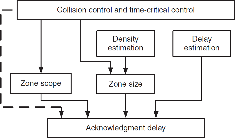
We compare derived analytical results with simulation results (shown in Fig. 6). The simulation setup is described in Section 5.1. In this set of experiments, the distance between the source and destination is set to 180 m and sensor nodes move at 20 m/sec. As shown in Fig. 6, PSGR's analytical result approximates the experimental result very well. Figure 6a plots the energy consumption. The small transmission range (i.e., less than 10 m) incurs high energy cost due to the poor network connectivity, and hence there are a large number of rebroadcasts at each hop. The energy consumption dramatically decreases as the transmission range increases, and reaches its minimum at R=15m. After that, as the packets can be routed for more hops before being dropped or arriving at the destination, the energy consumption moderately increases. Even though the energy cost is minimized at R = 15 m, it may not be a good choice considering the delivery rate shown in Fig. 6b. The delivery rate rapidly increases with the transmission range until before it hits 20 m. When R is larger than 30 m, both simulation and analytical results achieve at least 99% delivery rate. The transmission range should be chosen by considering both energy efficiency and delivery rate. Therefore, 20 m, 25 m, and 30 m are all reasonable choices for the transmission range.

Figure 6.

Analytical results for PSGR performance.

5. Performance Evaluation

To evaluate the performance of PSGR, we developed a simulator to test its sensitivity to various system factors (e.g., mobility and power saving (sleep) mode of sensor nodes, network density, number of sensor nodes, network traffic, and location error). Several state-of-the-art routing protocols, namely, flooding, IGF [2], GeRaf [39, 40], GPSR [20], and MSPEED [7] were included for comparison.

5.1. Metrics and Settings

We implemented the proposed PSGR, as well as counterpart routing protocols, in ns-2 (with the CMU wireless extensions). Similarly to [17, 20], we adopt IEEE 802.11b as the MAC layer protocol. The maximum transmission range of a sensor node, R_max, is set to 40 m [14]. The path loss factor for radio transmission, α, is set to 3. We extended the transmission power control module in ns-2 to capture the power consumption for dynamically adjusted radio transmission ranges. By default, 5 pairs of source and destination are simulated with a packet generation rate of 5 packets/sec at a source node. The locations of source and destition are randomly selected. For PSGR, we set the maximum number of rebroadcasts and the maximum number of bypassing hops both to 6, which is the same as the number of forwarding-region shifts in IGF [2]. According to [39, 40], we simulate GeRaf with four forwarding zones that divide the forwarding region evenly; the total times of transmissions allowed for a packet holder before dropping the packet is 10, which includes the messages used for triggering the acknowledgements in a forwarding zone, those for resolving collisions, and those for rebroadcasts when a communication void is encountered.

We simulate the mobility of sensor nodes using a sound random waypoint mobility model [37] in which the initial speed is chosen from a computed steady-state distribution, and all subsequent speeds are chosen from a configurable range [0, V_max] following a given speed distribution (a uniform speed distribution in our experiments). This approach generates stable sensor node movements, e.g., a fixed average speed and a fixed speed variance. Moreover, this model is orthogonal to the spatial network distribution created by the original random waypoint model, such that the spatial distribution of sensor nodes moving according to this model is nonuniform even though the nodes are initially placed uniformly inside the experiment region. Generally, a node randomly chooses a destination within the simulated field and a speed, and then moves to the destination from its current location at the chosen speed. Upon arriving at the destination, the node pauses for a configurable period, called pause time, before repeating the same process. In our simulation, the pause time is set to 0, so that the mobility of sensor nodes is totally controlled by varying the maximum moving speed of sensor nodes V_max (with a default value of 15 m/sec). Furthermore, we vary the node degree, the average number of neighbor nodes in the transmission area of a sensor node covered by R_max, from 5 to 20 to simulate the network with various degrees of node density. For each packet routing request, source and destination locations are randomly chosen within the simulated field.

Differently from the stateless routing protocols under examination, sensor nodes in GPSR have to periodically exchange up-to-date locations with their neighbors via beacon messages. We tested GPSR with different beacon intervals (i.e., 1.0 sec, 1.5 sec, and 3.0 sec), but show the results with a beacon interval of 3.0 sec only, as this setting consumes much less energy than the other two settings while maintaining a reasonable delivery rate and latency. Each simulation run lasted for 600 sec of simulated time. The results are obtained by averaging the performances over 25 runs of randomly generated movement traces or sleep traces. Table 2 summarizes the parameter settings in the simulation. The following three metrics are studied in our evaluation:

Energy consumption: the average amount of energy consumed by a packet routing request, including the energy cost of packet transmission and packet reception operations.

Delivery rate: the ratio of the number of successfully delivered packets to the total number of packet routing requests.

Latency: the average elapsed time for a successful packet delivery.

Table 2

Parameter settings

Parameters	Values	Parameters	Values
Max transmission range Rmax	(m)	40	Path loss factor α	3
Number of nodes	100	Simulation time (sec)	600
Field size (m2)	160 × 160	Max speed Vmax (m/sec)	0–30
Pause time (sec)	0	Node degree	5–20
Packet size (byte)	32	Number of trials	25

5.2. Basic Design of PSGR

We first study the basic design of PSGR by examining the prioritized acknowledgment scheme, resilience to the communication void, and provisioning of time-critical routing with different routing deadlines. Meanwhile, we consider the impact of network dynamics caused by the mobility of sensor nodes on the routing protocol. To simplify our discussion, we assume that the sensor nodes do not go to power saving mode in mobile networks. Later, in Section 5.6, we will consider the impact of power saving mode on geo-routing protocols in a stationary network.

5.2.1. Prioritized Acknowledgement

To isolate the impact on performance of the void communication problem from the prioritized acknowledgement mechanism, we only consider dense networks in this set of experiments (by setting node degree = 20) so that communication void regions rarely occur.

Figure 7 shows the performance of PSGR (under two different forwarding zone formation heuristics, DTD and M_DTD), IGF, GPSR, GeRaf and flooding algorithms. For a fair comparison, all algorithms under evaluation use R_max (i.e., 40 m) as the radio transmission range. Additionally, we plot the curves of PSGR with R = 30 m (obtained based on our analysis in Section 4) to show the further improvement obtained with a dynamic transmission range. The network dynamics is simulated by varying the maximum moving speed of sensor nodes, V_max, from 0 m/sec to 30 m/sec.

Figure 7.

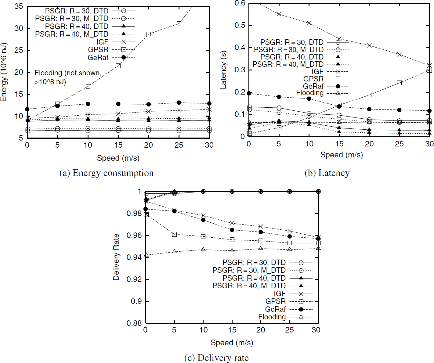
Heuristics for forming forwarding zones (node degree = 20).

Figure 7a compares the energy consumption of all routing algorithms. The flooding algorithm has a very high energy consumption (i.e., 3.7 × 10⁸nJ) that is not shown for clarity of the presentation. When the sensor nodes are static (V_max = 0 m/sec), all algorithms using R = 40 m except GeRaf have similar performance, whereas PSGR using R = 30 m is clearly better than the others. GeRaf performs poorly due to acknowledgement collisions occurring in the non-optimized forwarding zones. As the mobility of sensor nodes increases, the energy expense of GPSR rises dramatically since the increasing number of broken links causes more retransmissions. On the other hand, the impact of network dynamics on the stateless algorithms (i.e., PSGR, GeRaf, and IGF) is not that obvious. PSGR has the lowest and most stable energy consumption in all cases tested (whether using the maximum or the optimized transmission range). Between the two heuristics we adopt for forming forwarding zones in PSGR, DTD performs better than M_DTD since DTD was designed to minimize the number of forwarding hops.

Figure 7b compares the routing latency for all algorithms. IGF has an overwhelmingly longer latency than the other algorithms due to its long acknowledgment delay and small forwarding region. However, its routing latency decreases with increasing mobility, as more delivery failures are observed in a more dynamic network (see Fig. 7c) and the latencies for those dropped packets are not counted. GeRaf suffers from its ineffective collision resolution algorithm, which may take several tries before a successful packet forwarding [39]. GPSR outperforms all the other algorithms when the network is static, as routing decisions can be made directly based on cached state information. When the network becomes more dynamic, the latency of GPSR increases rapidly, as broken links cause more retransmissions and hence a longer delay at each hop. In dynamic networks, PSGR performs the best. Setting the radio transmission range to the maximum has a positive impact on latency, since the average number of relays during the routing is reduced. Furthermore, because of a shorter acknowledgement timer, PSGR-M_DTD performs better than PSGR-DTD.

Figure 7c shows the delivery rate of all algorithms. As the same technique is used for over-coming the communication void problem, PSGR-DTD and PSGR-M_DTD have a very minor difference in terms of the deliver rate. The flooding algorithm performs the worst; this is because a lot of packets are dropped in collisions. ⁵ GPSR has a worse performance than IGF and PSGR because of the inaccuracy of cached state information and the communication collisions caused by excessive beacon exchanges. IGF's delivery rate decreases as the network gets more dynamic. This can be explained as follows. The best PF, which is usually near the boundary of the packet holder's radio coverage area, is more likely to flee away owing to the long acknowledgement delay in IGF. As a result, the holder may not be able to hear from the fleeing PF, while other PFs probably could and thus drop their own acknowledgments. GeRaf also shows a decreasing delivery rate with increasing sensor node mobility, due to few forwarding zones and its inefficient collision resolution algorithm. We observed in the simulation that under a higher mobility, more collisions are incurred by GeRaf. On the contrary, the moving speed of sensor nodes has a positive impact on the delivery rate of PSGR, as the network dynamics leads to a higher chance of overcoming void regions. As shown in the figure, PSGR reaches a delivery rate of 100% when the sensor nodes move faster than 10 m/sec, whereas other algorithms perform no better than 98% in most cases.

5.2.2. Impact of Communication Void Problem

In this section, we investigate the resilience of PSGR to the communication void problem in a relatively sparse sensor network ⁶ For a fair comparison of this, and the rest of the experiments, we fix the transmission range R to 40 m in all the algorithms. The heuristic used in PSGR for prioritized acknowledgement is fixed to DTD. Two strategies for PSGR to overcome communication void regions, rebroadcast (labelled as PSGR:rebc) and bypass (labeled as PSGR:bypass), are examined separately. Figure 8 compares the performance of PSGR:rebc, PSGR:bypass, IGF, GeRaf and GPSR by varying the maximum moving speed of sensor nodes V_max from 0 m/sec to 30 m/sec.

Figure 8.

Communication void problem (node degree = 15).

Figure 8a shows the energy consumption of the compared algorithms. Again, the energy expense of the flooding algorithm is significantly higher than the others and thus is not shown. GPSR consumes more energy than IGF and GeRaf, which in turn perform worse than PSGR:rebc and PSGR:bypass. For PSGR, the bypass scheme has a higher energy cost than the rebroadcast; this is because each extra bypassing hop takes three transmissions (i.e., request, acknowledgement, and data packet forwarding), whereas a rebroadcast incurs one forwarding request only. Moreover, the rebroadcast tries to go across a void region in a straight line fashion (thus resulting in fewer hops) while the bypass takes extra hops to circumvent the void. Nevertheless, the superiority of the bypass is clearly demonstrated in Fig. 8b, where it has the best latency among all the algorithms. The bypass scheme is more time-efficient than the rebroadcast. PSGR:rebc works better in a more dynamic network because a potential forwarder may come into the void region sooner. Again, for the same reason explained earlier, GPSR's routing latency dramatically increases as the sensor mobility rises. Due to lower node density, IGF has an even longer routing latency (i.e., more than 1.0 sec), far exceeding the range of the y-axis. Finally, Fig. 8c shows the delivery rate. PSGR:bypass has the highest delivery rate in a static sensor network and remains almost constant regardless of the moving speed of sensor nodes. However, in a static network, PSGR:rebc has a slightly lower delivery rate than IGF and GeRaf, which look for PFs inside the holder's radio coverage area by shifting the forwarding region. The delivery rate of PSGR:rebc improves remarkably when sensor nodes increase moving speed.

5.2.3. Impact of Time-Critical Routing

In this section, we investigate the PSGR's ability to meet various routing deadlines by comparing it with MSPEED [7], a stateful time-critical routing algorithm. To be focused, we fix the network density by setting the node degree to 20 and use the rebroadcast scheme for overcoming communication voids. To simulate different traffic loads, we vary the number of traffic flows from 1 to 20. Each source node generates packets with a rate of 5 packets/sec. A source node randomly selects the routing deadline for its traffic flow from the range [0.3,1] sec, and packets originated by the same source node have the same routing deadline. In both PSGR and MSPEED, a packet is dropped when it misses its routing deadline. Moreover, to evaluate the effectiveness of time-critical routings, we exclude the routing failures caused by other factors (e.g., network dynamics, communication void problem and network disconnections). We consider both the network with stationary sensor nodes by setting V_max = 0 m/sec and the network with mobile sensor nodes by setting V_max = 15 m/sec. Since different traffic flows have different routing deadlines, the metric of average routing delay used in previous experiments is not informative to the performance of time-critical routings. Thus, this section employs the average delivery rate derived from all traffic flows to measure how well the time requirements are satisfied by PSGR and MSPEED.

The first experiment studies the scheduling policies ERDF and LSF in PSGR, labeled as PSGR:ERDF and PSGR:LSF. Figure 9a shows that with low and medium network traffic (i.e., fewer than 12 traffic flows) the two scheduling policies have similar performance, with PSGR:ERDF being slightly better. With increasing number of traffic flows, PSGR:LSF successfully delivers more packets than PSGR:ERDF. This is because ERDF gives higher priority to the packet that has less remaining time for reaching the deadline. Such packets are more likely to miss their deadlines during routing under a high network traffic. To show that the benefit gained by PSGR over MSPEED is not only because of a better scheduling policy, the remainder of this section will show the experimental results of PSGR:ERDF and that of MSPEED.

Figure 9.

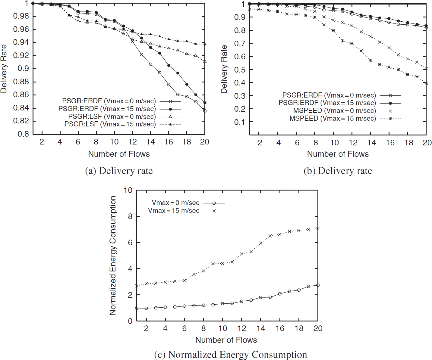
Time-critical routing (node degree = 20).

Figure 9b demonstrates that PSGR is able to deliver more packets to the destination than MSPEED with varying number of traffic flows. Moreover, the difference in their delivery rates increases when the network traffic becomes heavier. There are tow reasons for this. First, in MSPEED, a packet may be forwarded to a relay node that is not able to meet the routing deadline. In this case, the packet has to be re-routed (i.e., back-pressure re-routing), which prolongs the routing procedure and causes more deadline misses. Second, beacon message exchanges incurred by the stateful MSPEED protocol further intensify the network traffic, thus increasing the network delay and the scheduling delay and causing more routing failure. Figure 9c shows the normalized energy consumption (i.e., the ratio of energy consumption of MSPEED to that of PSGR). The larger the normalized energy consumption, the better energy-efficiency the PSGR achieves. The result demonstrates that for both stationary and mobile sensor networks, PSGR consumes less energy than MSPEED. The energy consumption ratio increases as the network traffic increases. In addition to the communication overhead incurred by the stateful routing itself, we believe that this trend is also caused by the increasing number of back-pressure re-routings in MSPEED (discussed in Section 2.2).

5.3. Network Density

This section evaluates the impact of network density on the performance of the compared algorithms. We set V_max to 15 m/sec to simulate a moderately dynamic network and vary the average node degree from 5 to 20 (by fixing the number of sensor nodes (i.e, 100) and scaling the experiment field from 317 × 317 m² to 160 × 160 m² correspondingly). For the remaining experiments, to be focused, we do not consider time-critical routing, so that traffic flows are not constrained by routing deadlines.

As shown in Fig. 10a, the energy expense of all algorithms is reduced with increasing network density. When the network is sparse, the energy conserved by PSGR:rebc against IGF or GPSR is up to 50%. In contrast, because of a higher recovery cost from the communication void, PSGR:bypass shows improvement against GPSR and IGF of less 20% (when node degree = 5) to 30% (when node degree = 15). GPSR performs the worst due to its high overhead for maintaining neighbors' states.

Figure 10.

Network density (V_max = 15 m /sec).

Figure 10b plots the routing latency for all algorithms. Again, IGF has a much longer routing latency than all others (i.e., longer than 0.48 sec and up to 17 sec) so it is not shown in the figure for the clarity of the presentation. PSGR:bypass performs best under the various settings of network density. For example, PSGR:rebc takes longer to deliver a packet because it successfully delivers more packets than other algorithms (i.e., up to 17% more than PSGR:bypass, IGF and flooding, and 45% more than GPSR and GeRaf as shown in Figure 10c) thus incurs more network traffic. Figure 10b shows that increased network density results in a decreasing latency for PSGR:rebc, which eventually outperforms the other algorithms, except PSGR:bypass, when network degree is higher than 15.

5.4. Scalability

In this section, we examine the scalability of PSGR and other counterpart protocols by increasing the number of sensor nodes deployed in a proportionally enlarged field (i.e., the network density is fixed such that node degree = 20). We choose a moderately dynamic network with the maximum moving speed of sensor nodes equal to 15 m/sec.

Two observations can be made from Fig. 11a. First, the energy consumption of all algorithms increases with increasing number of nodes (and field size), since the average path length of the packet routing increases. Second, the volunteer forwarding based stateless routing protocols (i.e., PSGR, GeRaf, and IGF) demonstrate better scalability over the stateful GPSR, which incurs more beacon exchanges to maintain the cached state information as the number of nodes increases.

Figure 11.

Scalability (V_max = 15 m/sec, node degree = 20).

Figure 11b compares the routing latency. The latencies of IGF and GPSR increase rapidly as the network grows. For IGF, this is due to the cumulative cost of routing packets for a longer distance. For GPSR, in addition to the cumulative cost due to the longer distance, there are more broken links to be fixed along the routes. On the other hand, GeRaf does not incur prolonged routing latency, since we regulate the maximum number of control packets (i.e., 10) for each packet holder. It is encouraging to note that PSGR demonstrates good scalability to a large network. The routing latency of PSGR increases only slightly as the routing distance is increased. As for the delivery rate, one would expect that as the routing distance gets longer the probability of failing in routing a packet to the destination increases. This is true for GeRaf, IGF, and GPSR as shown in Fig. 11c. However, thanks to the robust solutions to the communication void problem, PSGR is able to maintain a high delivery rate in all cases tested.

5.5. Resilience to Location Errors

Geo-routing protocols require all sensor nodes to be location-aware. However, high-precision location information is difficult or expensive to obtain. Moreover, errors are not avoidable in many positioning/localization techniques. This section examines the impact of location errors on the performance of compared routing protocols. We fix the network density by setting node degree to 20 and the mobility of sensor nodes by setting V_max to 15 m/sec. Location errors are independently introduced to the (x, y) coordinates of a sensor node by randomly adding a value drawn from [−µ*R_max, µ*R_max], where µ is a variable to control the degree of errors ⁷ . Meanwhile, we redefine a successful delivery as a data packet reaching a distance within (1 − µ) * R_max of the destination. Figure 12 shows the performance of routing algorithms with µ varied from 10% to 50%.

Figure 12.

Location errors (V_max = 15 m/sec, node degree = 20).

As expected, Fig. 12a shows that the energy consumption increases with location error for all algorithms except flooding. Both PSGR:rebc and PSGR:bypass algorithms consume the least energy for µ < 0.4; when the location inaccuracy is more than 40% of R_max, PSGR:bypass consumes more energy than IGF. This is because the imprecision in location can result in more hops than necessary for the bypass scheme, since forwarding nodes selected may not always be the best nodes. The same reason also explains Fig. 12b, where PSGR:bypass incurs a longer latency for highly inaccurate locations.

As expected, the delivery rate is lower with less accurate location information for all routing algorithms except the flooding (see Fig. 12c). The impact on GPSR and IGF is most significant. In order to overcome void regions, GPSR has to construct the underlying network planar graph based on the geographical locations of sensor nodes. With inaccurate location information, the constructed planar graph cannot serve its purpose well, resulting in loops during routing. For IGF, we believe this is because the small forwarding region used by IGF excludes the best PF but likely selects some node outside the real forwarding region. With a much larger forwarding region, PSGR and GeRaf have better tolerance to this problem.

5.6. Power Saving (Sleep) Mode

In this section, we study the impact of power saving (sleep) mode on geo-routing protocols. Here we consider a stationary (non-mobile) sensor network in which some or all sensor nodes are periodically switched between a sleep mode and an active mode for energy conservation. Even though the sensor nodes are stationary, the network topology is still dynamic. Two parameters, i.e., ratio of sleep nodes and maximum sleep period (i.e., t_max) are used to control the network dynamics. The ratio of sleep nodes denotes the percentage of sensor nodes in sleep mode at a given time; this has an impact on the network density. The maximum sleep period specifies the period of time a sensor node stays in the sleep mode, which determines the frequency of network topology transients. Specifically, our simulation randomly selects S sensor nodes such that $\frac{S}{N}$ = ratio of sleep nodes and inactivates these nodes for t seconds, where t is randomly selected from [0, t_max]. After t seconds, the nodes are re-activated and the same process is repeated. In this process, the nodes currently engaged in packet routing (i.e., the holders, the PFs and the bypassing PFs) are not selected for inactivation to avoid packet losses. In order to simulate the network dynamics, we vary the ration of sleep nodes from 0 to 1 with a default value of 0.4 and t_max from 50 ms up to 1000 ms with a default value of 100 ms.

Figures 13a through 13c depict the energy consumption, routing latency, and delivery rate of the compared routing protocols with varying ratio of sleep nodes. The energy consumption of flooding drops dramatically with increasing numbers of sleep nodes, since fewer nodes are involved in routing. The stateless routing algorithms (i.e., GeRaf, IGF, and PSGR) consume more energy as the number of inactivated nodes increases (and the network connectivity decreases). Their energy consumption and routing latency eventually drop off as the number of inactivated nodes continues to increase (i.e., decreasing network density). GPSR shows a similar trend but is affected more severely since much effort is required for each packet forwarding given the stale cached state information. In Fig. 13c, all algorithms show decreasing delivery rates, as fewer sensor nodes are activated (and the network connectivity decreases).

Figure 13.

Power Saving Mode.

The remaining figures (Figs. 13d through 13f) study the compared routing algorithms by varying the sleep period of nodes from 50 ms to 1000 ms with 40% of sensor nodes sleeping at any given time. All stateless routing algorithms show stable energy consumption and delivery rates, regardless of the dynamics of the sensor network. On the other hand, the stateful GPSR has a noticeably decreasing energy consumption and routing latency when the network becomes more stable (i.e., with a longer sleeping time), which improves the freshness of the cached state information at sensor nodes, thus in turn increases its delivery rate.

6. Summary

In this paper, we presented a novel and robust stateless geo-routing protocol, namely, PSGR, for large-scale location-aware wireless sensor networks. PSGR, built upon a carefully crafted priority-based acknowledgement mechanism, removes the requirements for knowledge about the network topology and states (e.g., locations and links) of neighbor nodes. The priority-based acknowledgement mechanism exploits two crucial concepts that contribute significantly to the novelty, robustness and high performance of PSGR:

dynamic zone formation (based on sensor node density estimated on-the-fly); and

autonomous acknowledgements that avoid collisions.

Profound analysis of these concepts empowers PSGR to effectively avoid acknowledgement collisions and thus optimize the energy efficiency and forwarding latency. In addition, we employ two stateless strategies, namely rebroadcast and bypass, to address the communication void problem in PSGR. These two strategies favor responsiveness and energy efficiency, respectively, and work complementarily under various network scenarios. Moreover, we show that volunteer forwarding is naturally more suitable for supporting time-critical routing, so we designed the first time-critical control mechanism for volunteer forwarding; this empowers PSGR with the ability to deliver packets with different routing deadlines on time. Another important contribution made by this work is the analytical model developed for energy consumption and delivery rate. The analysis provides important insights on selecting transmission range and is very helpful for planning and deployment of large scale wireless sensor networks. Finally, an extensive performance evaluation was conducted to compare the performance of PSGR with state-of-the-art geo-routing protocols for wireless sensor networks, including flooding IGF [2], GeRaf [39, 40], GPSR [20], and MSPEED [7]. Various network conditions were simulated and tested on the compared protocols, including network dynamics (caused by sensor node mobility and power saving mode), network density, network size, and network traffic. We also examined the resilience of PSGR to the inaccuracy of location information (which is critical in making geo-routing decisions). To the best of our knowledge, this is the most extensive performance evaluation conducted in comparison of stateless geo-routing protocols. Simulation results show that PSGR exhibits superior performance in terms of energy consumption, routing latency, and delivery rate, and soundly outperforms all the compared protocols. For static or less dynamic sensor networks, PSGR with the bypass strategy is the best choice; it is highly competitive to GPSR, which is specifically designed for such scenarios. In a dynamic sensor network, PSGR with rebroadcast is the preferred technique.