Sage Journals: Discover world-class research

Abstract

Sensor nodes in a distributed sensor network can fail due to a variety of reasons, e.g., harsh environmental conditions, sabotage, battery failure, and component wear-out. Since many wireless sensor networks are intended to operate in an unattended manner after deployment, failing nodes cannot be replaced or repaired during field operation. Therefore, by designing the network to be fault-tolerant, we can ensure that a wireless sensor network can perform its surveillance and tracking tasks even when some nodes in the network fail. In this paper, we describe a fault-tolerant self-organization scheme that designates a set of backup nodes to replace failed nodes and maintain a backbone for coverage and communication. The proposed scheme does not require a centralized server for monitoring node failures and for designating backup nodes to replace failed nodes. It operates in a fully distributed manner and it requires only localized communication. This scheme has been implemented on top of an energy-efficient self-organization technique for sensor networks. The proposed fault-tolerance-node selection procedure can tolerate a large number of node failures using only localized communication, without losing either sensing coverage or communication connectivity.

Keywords

Connected Dominating Set Fault Tolerance Localized Communication Network Organization Sensor Networks Topology Control

1. Introduction

Wireless sensor networks can be deployed to provide continuous surveillance and monitoring over a designated area of interest [2,7,19,22]. Many wireless sensor nodes have low cost and small form factors [1, 2, 7]; therefore, they can be deployed in large numbers with high redundancy. A typical example of such low-cost sensor nodes is the set of Berkeley motes from Crossbow Technology [33]. Since nodes are deployed in a redundant fashion, not every node in the network needs to be continuously active for sensing and communication. The operational lifetime of sensor networks can be increased by network organization schemes for topology control, where only a subset of nodes are kept active, while the other nodes are kept in a sleep state or a power-saving mode [14,27,31]. Fewer active nodes also place less demand on the limited network bandwidth.

Since a wireless sensor network should ideally perform surveillance tasks in an unattended manner, it needs to operate as long as possible, even when many sensor nodes fail. This motivates our work on fault-tolerant self-organization. Most recent work aims to provide fault tolerance in the deterministic deployment of sensor nodes [9,17,21,24]. Much less attention has been devoted to distributed protocols that can replace failing nodes in the network with spare nodes. Failing sensor nodes result in coverage loss and breakage in communication connectivity, hence there is a need for a distributed node replacement protocol and self-organization scheme that designates nodes as fault tolerance (spare) nodes. Such a scheme should be fully distributed such that it can be scalable for a large number of nodes. It should only require localized communication to select backup nodes for fault tolerance, and it should not rely on a centralized server to identify and replace faulty nodes.

This paper presents redundancy analysis and a distributed self-organization scheme that ensures communication connectivity and sensing coverage when nodes fail, either sequentially or simultaneously. We first present analytical results to characterize the extent of redundancy needed for fault tolerance. We then describe a distributed scheme that achieves fault tolerance by selecting fault tolerance nodes that can replace failing nodes. The proposed distributed approach uses only single-hop or restricted-hop neighborhood information to select fault tolerance nodes. We show that the proposed approach provides communication connectivity and sensing coverage even when up to Ω nodes fail, where Ω is a user-defined parameter.

The paper is organized as follows. In Section 2, we briefly describe related prior work. In Section 3, we present the background and assumptions used in this paper. Section 4 describes fault tolerance for communication connectivity. Section 5 addresses fault tolerance for sensing coverage. We present simulation results for the proposed distributed self-organization technique in Section 6. Section 7 concludes the paper and outlines directions for the future work.

2. Related Work

Energy-efficient self-organization in wireless sensor networks has received considerable attention in the literature [13,16,20,23,26,29]. Energy considerations have been used to find a set of (active) nodes that can form a backbone for the network. Selection of these backbone nodes can be achieved by heuristics described in [3,4,25,28] based on the concept of a connected dominating set, where the distributed algorithm proposed in [3] has the best message complexity. The selection of active nodes to guarantee both sensing coverage and communication connectivity has been studied in [14,27,31]. A recent approach distinguishes connectivity from sensing, and determines the configuration of the nodes with both communication connectivity and sensing coverage as considerations [27].

Fault-tolerance in distributed sensor networks has received relatively less attention [9,17,21,24]. Problems studied include the characterization of sensor fault modalities [17,24], faulttolerance in multiple-sensor fusion [21], and reliable information dissemination [9]. Recent work on fault-tolerance in wireless sensor networks can be categorized as being focused on fault detection [6,10,12] or fault-tolerant operations [15,30]. In [10], the authors present various fault tolerance techniques at different levels, including the physical layer for communication, the hardware components of a sensor node, system software such as the embedded operating system, middleware, and application. In [12], the authors consider faults in node sensor measurements and develop a distributed Bayesian algorithm to detect and correct such faults. [6] also addresses a similar fault detection problem, and presents a crash identification mechanism. In [30], the authors show that a sensor network with n nodes is asymptotically connected if each node is directly connected to at least 5.1774 log n neighboring nodes. [15] shows that for a wireless sensor network with n nodes, the connectivity probability with up to k failing nodes is at least e^eα when the transmission radius r satisfies nπr²  ln n + (2k − 1) ln ln n − 2ln k! + 2α. Recently, in [11], a protocol has been proposed for event detection in sensor networks, which is able to handle both natural and malicious node failures in sensor networks. However, most prior work has not characterized the redundancy necessary for fault tolerance, and no distributed self-organization protocol has directly considered this issue.

3. Preliminaries

3.1. Assumptions

The discussion in this paper is based on the following assumptions:

The ad hoc sensor network is deployed with a sufficient number of nodes such that the network is connected. All sensor nodes have the same maximum communication range r_c and maximum sensing range r_s.

We represent the surveillance field by a 2D grid, whose dimension is given as X × Y. Let G = {g₁,g₂,…,g_m} be the set of all grid points, and m=|G|=XY.

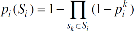
We use S to denote the set of n sensor nodes that have been placed in the sensor field, i.e., |S| = n. A node with id k is referred to as s_k(s_k ∊ S, 1  k  n). Let d^k_i be the distance between the grid point g_i and the sensor node s_k. In a graph model G(V, E) for a set S of nodes, we use the vertex ν ∊ V in the graph model interchangeably with its corresponding node s ∊ S. The set of edges E denotes the connectivity between nodes.

We model sensing coverage using the probability p^k_i that a target at grid point g_i is detected by a node s_k:

p_{i}^{k} = {\begin{cases} e^{- α d_{i}^{k}}, & if d_{i}^{k} \leq r_{s}; \\ 0, & otherwise, \end{cases}

(1)

where α is a parameter representing the physical characteristics of the sensor. The model conveys the intuition that the closer a location is to the node, a higher signal-to-noise ratio is expected, resulting in a higher confidence level that a target at that location is detected. Areas beyond the maximum sensing range r_s are then considered to be too noisy for the sensor node to determine if there is a target. The sensing model is only used for coverage evaluation during active node selection; alternative sensing models can also be easily considered. Assume that S_i is the set of nodes that can detect grid point g_i; thus the detection probability for grid point g_i is evaluated by Equation (1) as

p_{i} (S_{i}) = 1 - \prod_{s_{k} \in S_{i}} (1 - p_{i}^{k})

(2)

3.2. Coverage- and Connectivity-centric Selection of Active Nodes for Self-organization

In this paper, we focus on the fault tolerance problem in the topology control of ad hoc sensor networks. We assume that a network organization scheme is provided to the sensor network. Network organization can be achieved by using techniques described in [14,27,31], which select a subset of active nodes as a backbone for communication connectivity and/or sensing coverage. The failure of these active nodes can result in loss of connectivity and/or loss of sensing coverage. We use S_a (S_s) to denote the set of active (sleeping) nodes determined by such active nodes selection algorithms, and the following discussion assumes that S_a and S_s have already been determined. We consider the threshold p_th to be a parameter underlying a successful sensing coverage over the sensor field. The following conditions are implicitly satisfied: 1) $\forall g_{i} \in G$ and S_i ⊆ S_a, p_i(S_i p_th; 2) ∀s_k ∊ S_a is connected.

In [31], we have shown that the problem of selecting a subset of nodes as a backbone for both sensing coverage and communication connectivity is NP-complete. We have also presented the token-based coverage- and connectivity-centric active node selection (CCANS) protocol that achieves self-organization with a subset of active nodes, which are responsible for both the coverage and the connectivity. In this section, we first review the token-based CCANS protocol for energy-efficient self-organization. We then describe the problem of providing fault tolerance to active backbone nodes in the following sections. The proposed fault-tolerant self-organization technique is general, and it can also be used with other self-organization protocols. CCANS is used in this paper as a vehicle to evaluate the proposed method.

3.3. Token-based CCANS Protocol

There are three types of messages used in this protocol, namely HELLO, STATE, and UPDATE. These messages contain such fields as tokenid and srcid which enables the token to control the execution of the sensing coverage evaluation and connectivity checking. There are three possible states for all nodes, namely UNSET, SLEEP and ACTIVE. Initially, all nodes are in UNSET state with their tokenid = −1, i.e., no token has been given to them for the execution of the CCANS algorithm. There are two stages in the CCANS protocol, namely Stage 1 for node sensing coverage evaluation, followed by Stage 2 for node state and connectivity checking. The node with the assigned token is referred to as the token node and all other nodes either collect messages sent from the token node or perform no action. In Stage 1, the current token node evaluates the coverage within its sensing area versus the coverage within its sensing area contributed by its neighbors. It chooses the state ACTIVE if its sensing area is not fully covered by its neighbors, otherwise it chooses the state SLEEP. However, this state decision is not final until the connectivity checking and coverage re-evaluation are completed in Stage 2. One node is pre-selected as the start node by the base-station to initiate the execution of the CCANS algorithm for finding a subset of active nodes.

The token passing procedure is designed to reduce the execution time of the algorithm by expanding the global sensing coverage as much as possible [31]. Consider an arbitrarily chosen node s_k. s_k gets the token for execution of the CCANS algorithm when id(s_k) = tokenid. If tokensrc(s_k) = −1, then s_k sets tokensrc(s_k) = srcid; this is set only once. Therefore, every node knows its token source and is able to pass the token back to its token source when it completes CCANS Stage 2. If s_k is the start node, then initially tokensrc(s_k) = id(s_k) ≠ −1. At the time when the token is passed back to s_k, if s_k has no UNSET neighbors, it executes Stage 2 of the distributed CCANS procedure to find its own final state decision; then the distributed CCANS procedure terminates. As an example, Fig. 1 (a) illustrates token passing for an example sensor network with four sensor nodes, s₁, s₂, s₃, and s₄, where s₁ is the start node. The steps in this example are as follows:

(a)
Initially all nodes are in UNSET state and s₁ is the start node.
(b)
s₁ has completed CCANS State 1 and passes the token to s₂.
(c)
s₂ has completed CCANS Stage 1 and passes the token to s₃.
(d)
s₃ has no more UNSET neighbors and it has completed CCANS Stage 2, therefore s₃ passes the token back to s₂.
(e)
s₂ still has UNSET neighbors so s₂ passes the token to s₄.
(f)
s₄ has no more UNSET neighbors and it has completed CCANS Stage 2, therefore s₄ passes the token back to s₂.
(g)
s₂ has no more UNSET neighbors and it has completed CCANS Stage 2, therefore s₂ passes the token back to s₁.
(h)
s₁ has no more UNSET neighbors and it has completed CCANS Stage 2. Since s₁ is the start node, all nodes have made the state decision, and CCANS terminates.

Fig. 1(b) shows the sequence of the token source in terms of node id during the execution of the distributed CCANS procedure for the example shown in Fig. 1 (a). The CCANS procedure requires only constant rounds for message exchange in both stages [31]. Let Δ be the maximum node degree in the graph corresponding to the sensor network. The connectivity checking procedure in CCANS has a time complexity of O(Δ²) per node, and this is carried out independently by each node. Since the sensing coverage evaluation is carried out per grid point for all nodes in the neighborhood, the time complexity of the sensing coverage evaluation in CCANS is O(mΔ), where m is the number of grid points representing the sensor field. Therefore, the overall time complexity for the CCANS procedure per node is O(mΔ + Δ²). The complexity depends only on the maximum degree of a node and the grid granularity of the sensor field. As shown in [31], the CCANS protocol always terminates and achieves self-organization. The completion of the distributed CCANS procedure can be easily notified to the base station.
3.4. Fault-tolerant Self-organization

In this paper, we focus on fault-tolerant self-organization, where both the sensing coverage and the connectivity are preserved with support from the designated fault tolerance (FT) nodes when active nodes fail. We refer to this as the fault-tolerance-nodes-selection (FTNS) problem. The proposed distributed FTNS algorithm is executed after S_a and S_s are determined, where a set S_t of nodes is designated to be FT nodes (backup nodes for active nodes). These FT nodes provide fault tolerance for the existing active nodes. They need not be active unless the active nodes that they are supporting fail. They can run in a power-saving mode and periodically query whether the active nodes are still alive using very limited bandwidth.

Figure 1

(a) Example of token passing in the distributed CCANS procedure. (b) Token passing sequence for the example in Fig. 1 (a).

Note that simultaneous failures of nodes in S_a and S_t may result in loss in sensing coverage or breakage in communication connectivity since FT nodes are not backed up by nodes in S_t. However, if only FT nodes fail or FT nodes and their non-neighboring active nodes fail, the sensing coverage and communication connectivity are still guaranteed. Furthermore, the proposed distributed algorithm can be applied in a repeated manner to select more FT nodes for the previously selected FT nodes.

We assume that the number of nodes initially deployed in the sensor field is sufficient to achieve fault-tolerant operations, i.e., we have enough sleeping nodes available to select as FT nodes. Some observations and additional definitions are listed below:

It is trivial to see that if all failing nodes are sleeping nodes, the existing active nodes can tolerate the failure of up to |S_s| nodes.

We define the maximum number of active nodes that can fail simultaneously without losing sensing coverage or communication connectivity as the degree of fault tolerance (DOFT), denoted by Ω (Ω  1).

The nodes that are selected from the set of sleeping nodes to obtain a Ω-DOFT wireless sensor network are referred to as Ω-fault-tolerant (Ω-FT) nodes. We denote the set of Ω-FT nodes as $S_{t}^{Ω}$ .

Let $S_{t}^{0} = ϕ and S_{a}^{Ω} = S_{t}^{Ω} \cup S_{a}$ . It follows that $S_{a}^{Ω}$ provides a solution to the Ωj-DOFT FTNS problem. In other words, a Ω-DOFT FTNS-derived sensor network is still connected and provides undiminished coverage of the surveillance area if any Ω active nodes fail.

4. Connectivity-Oriented Fault Tolerance

In this section, we focus on the analysis of fault tolerance for communication connectivity. The discussion of fault tolerance for sensing coverage is presented in next section.

4.1. An Upper Bound on the Number of Fault Tolerance Nodes

We first consider the case of 1-DOFT, i.e., Ω = 1. Let N_k be the set of neighbors for s_k, $N_{k}^{a}$ be the set of active neighbors, and $N_{k}^{s}$ be the set of sleeping neighbors. Let Δ_k be the number of neighboring nodes for s_k, $Δ_{k}^{a}$ be the number of active neighboring nodes for s_k, and $Δ_{k}^{s}$ be the number of sleeping neighboring nodes for s_k. In other words, $Δ_{k} =∣ N_{k} ∣, Δ_{k}^{a} =∣ N_{k}^{a} ∣$ and $Δ_{k}^{s} =∣ N_{k}^{s} ∣$ . It is trivial to see that ∀s_k ∊ S, Δ_k  1 otherwise S is not connected. Thus communication connectivity is not affected if any node in S_s fails. This is also true if multiple nodes in S_s fail. Therefore, any number of sleeping nodes in S_s can fail either sequentially or simultaneously. This implies that only active nodes need to be considered as failing nodes for the analysis of connectivity fault tolerance.

It can be seen that, if ∃s_k ∊ S such that Δ_k = 1, then Ω-DOFT (Ω  1) cannot be achieved for the network since when this neighbor node of s_k fails, s_k is disconnected from the rest of the network [32]. For any wireless sensor network with S_a (S_a ≠ φ), ∀s_k ∊ S, s_k is connected to at least one node in S_a, i.e., Δ_k^a  1. Therefore, Δ_k  Δ_k^a  1. In a sensor network with S_a as a backbone for both sensing and communication, if s_k ∉ S_a, i.e., s_k is a sleeping node, we can expect Δ_k > 1 due to the need for sensing coverage; otherwise an active node must be located expect at the same location as s_k. This observation leads to a lower bound on the node density required in the sensor field for fault tolerance. This lower bound can be used as a necessary condition for the fault-tolerant sensor node deployment.

Consider a total of n nodes with communication radius as r_c each in a sensor field with area A. In order to achieve Ω-DOFT (Ω  1), a lower bound on the total number of nodes n in the sensor field is given by: $n \geq \frac{3 A}{π r_{c}^{2}}$ . The proof, which can be found in [32], is straightforward and is therefore omitted. For example, consider the extreme case of $A = π r_{c}^{2}$ . For this case, we must have n  3. This is obviously true since if there are only two nodes, neither of them can fail. In the following discussion, we assume that the initial sensor deployment has provided a sufficient number of nodes for fault tolerance. Our goal is to designate extra sleeping nodes as back-up nodes, i.e., FT nodes, to provide fault tolerance when currently-selected active nodes fail. We also need to minimize the number of FT nodes. Before we present bounds on the number of FT nodes needed to achieve Ω-DOFT, we prove the following theorem.

Theorem 1. Let s_k ∊ S be a node in the sensor network. Let the region that lies within the communication range r_c of s_k be A_k∗ and let S∗ be the set of nodes within A_k∗. Assume that all nodes in S∗ are connected to each other, i.e., ∀s_p, s_j ∊ S, there exists a routing path from s_i to s_j. In order to ensure communication connectivity between the nodes in S∗ if s_k fails, it is sufficient to have 10 nodes (not counting s_k) in A_k∗.

Proof. Let G(V, E) be the connected graph representing S∗, i.e., | V | = | S∗ |, ν_k is the vertex representing s_k ∊ S, and ∀u, ν ∊ V, (u, ν) ∊ E if d(u, ν)  r_c. Let G_c(V_c, E_c) be a subgraph corresponding to a connected-dominating-set (CDS) of G [3, 4, 8, 25, 28]. We first derive an upper bound on the number of vertices needed for a CDS. The circular area A_k∗ with radius r_c can be divided into six sectors, denoted by A₁, …, A₆ in Fig. 2 (a). Each sector A_i (1  i  6) has an opening angle of $\frac{π}{3}$ . From Fig. 2 (a), the nodes in S∗ can be located in one or multiple sectors, corresponding to the vertices in V in these sectors. Excluding equivalent cases due to symmetry, we list all possibilities for the locations of the vertices in Fig. 2 (b).

Case 1: All vertices are located in the same sector. Assume this sector is A₁ as shown in Fig. 2 (b) $a$ . Obviously, for any two vertices ∀u, ν ∊ V within A₁, d(u, ν)  r_c, which includes the case where u and ν can be located at the sector boundaries. We can simply let V_c = {u} where u is an arbitrary chosen vertex. Therefore, |V_c| = 1. For example, if an active node s_k has only two neighbors in one sector, where there are a total 3 nodes within the communication region of s_k. Fault tolerance can be achieved for the failure of s_k because one of its two neighbors can be designated as a FT node.

Case 2: All vertices are located within two sectors. There are three possibilities for the sectors A₁ and A₂, as shown in Fig. 2 (b) $b$ , 2(b) $c$ , and 2(b) $d$ , respectively. Since G is connected, ∃(u, ν) ∊ E such that u is in A₁ and ν is in A₂. Moreover, ∀u_i ∊ A₁, ∃(u, u_i) ∊ E and ∀u_i ∊ A₂, ∃(u, u_i) ∊ E. Therefore, V_c = {u, ν} is a CDS of G and | V_c|  2.

Case 3: All vertices are located within three sectors. There are four possibilities for the sectors A₁, A₂, and A₃, as shown in Fig. 2 (b) $e$ , 2(b) $f$ , 2(b) $g$ , and 2(b) $h$ , respectively. Let u be an arbitrarily-chosen vertex in A₁. Since G is connected, ∃(u, ν) ∊ E such that ν is either in A₂ or in A₃. Without loss of generality, assume that ν is in A₂. Similarly, for w ∊ A₃, ∃(w, x) ∊ E such that x is either in A₁ or in A₂. Therefore, V_c = {u, ν, w, x} is a CDS of G and | V_c|  4.

Case 4: All vertices are located within four sectors. There are three possibilities for the sectors A₁, A₂, A₃, and A₄ as shown in Fig. 2 (b) $i$ , 2(b) $j$ , and 2(b) $k$ , respectively. Divide these four sector areas into two groups where one group has three sectors and the other group has one sector. Assume that A₁, A₂ and A₃ are in one group the other group contains A₄. From Case 2, ∃(u, ν) ∊ E, where u is in A₄ and ν is in A₁, or A₂ or A₃. Furthermore, from the proof for Case 3, ∃V₁ = {w₁, w₂, w₃, w₄}, where V₁ is a CDS for vertices in A₁, A₂ and A₃. Therefore, V_c = {u, ν, w₁, w₂, w₂, w₄} is a CDS of G and | V_c |  6.

Case 5: All vertices are located within five sectors. There is only one possibility for the sectors A₁, A₂, A₃, A₄, and A₅ as shown in Fig. 2 (b) $1$ . Similar to the proof for Case 4, we divide these five sector areas into two groups where one group contains any four of these five sectors and the other group contains the remaining sector. Assume that A₁, A₂, A₃, A₄ are in the one group and A₅ is in the other group. From Case 2, ∃(u, ν) ∊ E, where u is in A₅ and ν is in A₁, or A₂, or A₃, or A₄. Furthermore, from the proof for Case 4, ∃V₁ = {w₁, w₂, w₂, w₃, w₄, w₅, w₆}, where V₁ is a CDS for vertices in A₁, A₂, A₃ and A₄. Therefore, V_c = {u, ν, w₁, w₂, w₂, w₃, w₄, w₅, w₆} is a CDS of G and | V_c |  8.

Case 6: Vertices are located in all six sectors. There is only one possibility for the sectors A₁, A₂, A₃, A₄, A₅, and A₆ as shown in Fig. 2 (b) $m$ . Similar to Case 3 and Case 4, we divide these six sectors into two group where one group contains five sector areas and the other group contains one sector area. Assume that A₁, A₂, A₃, A₄, A₅ are in the one group and A₆ is in the other group. From Case 2, ∃(u, ν) ∊ E, where u is in A₆ and ν is in A₁, or A₂ or A₃ or A₄ or A₅. Furthermore, from Case 5, ∃V₁ = {w₁, w₂, w₃, w₄, w₅, w₆, w₇, w₈}, where V₁ is a CDS for vertices in A₁, A₂, A₃, A₄ and A₅. Therefore, V_c = {u, ν, w₁, w₂, w₂, w₃, w₄, w₅, w₆, w₇, w₈} is a CDS of G and | V_c |  10.

Figure 2

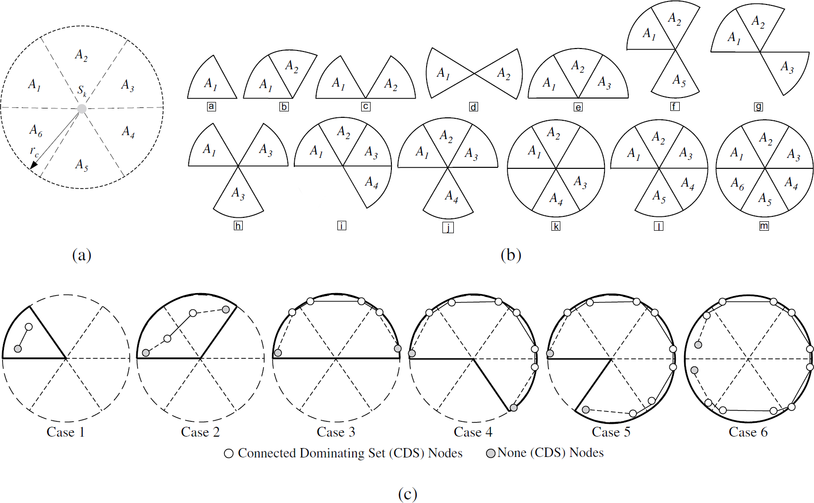
Illustration of the proof of Theorem 1: (a) A node&s communication region can be divided into six sectors with an opening angle of π/3. (b) Proof of Theorem 1: All possibilities of vertices locations. (c) Illustration of the six cases corresponding to Theorem 1.

The nodes corresponding to V_c thus keep all nodes in S∗ connected even when s_k fails. Therefore, the maximum number of required FT nodes for s_k is 10.

Figure 2(c) illustrates each of the six cases discussed in Theorem 1. Based on Theorem 1, we can derive an upper bound on the number of FT nodes needed within the communication region of an arbitrarily-chosen node. Assume that N_k is the set of neighbor for s_k ∊ S. Consider the special case where S = N_k ∪ {s_k}, i.e., all nodes in S\{s_k} are neighbors of s_k. Suppose the nodes in N_k are not connected. When s_k fails, ∃s_i, s_j ∊ N_k such that no routing can be formed between s_i and s_j. Thus fault tolerance can only be achieved if there is sufficient node density in the network. Let Γ_k be the number of FT nodes required for an arbitrarily-chosen node s_k in a 1-DOFT sensor network. Next we present a sufficient condition relating fault tolerance with Γ_k in the following theorem.

Theorem 2. The network is 1-DOFT with respect to the failure of any node $s_{k} \in S_{a} i f \forall_{s_{k}} \in S_{a}$ , the nodes in N_k are connected and Γ_k  10.

The proof of Theorem 2 is given in the appendix. Note that we need to have Γ_k = 10 only when s_k has no active neighbors, i.e., $Δ_{k}^{a} = 0$ . This is shown as Case 6 in Fig. 2 (c). Since S_a as a backbone is a non-empty set that connects all nodes, Γ_k = 10 needs to be 10 only if | S_a | = 1 and S_a = {s_k}. This means that all nodes are deployed within s_k&s communication region and only s_k is active. Generally, we have $\forall s_{k} \in S_{a}, ∣ Δ_{k}^{a} ∣\geq 1$ since |S_a| > 1, which implies the following corollary [32], which is proven in the appendix.

Corollary 1. When the number of active nodes is greater than one, i.e., |S_a| > 1, the sensor network is 1-DOFT with respect to the failure of any node s_k ∊ S_a if $\forall s_{k} \in S_{a}$ , N_k is connected and there are 9 or more FT neighboring nodes for s_k.

Corollary 1 shown that $Δ_{k}^{a}$ is a measure of the communication connectivity support provided by the active neighbors of s_k when s_k fails. In fact $Δ_{k}^{a} > 0$ implies that there exists built-in fault tolerance for s_k. The fault tolerance provided by the active neighbors in $N_{k}^{a}$ decreases the maximum number of FT nodes needed when s_k fails. Note that the above is true only for Ω = 1 since when Ω > 1, nodes in $N_{k}^{a}$ may also fail at the same time when s_k fails. Both Theorem 2 and Corollary 1 assume that when s_k ∊ S_a fails, the selected FT nodes for s_k do not fail. Since FT nodes are selected to provide fault tolerance for active nodes in S_a, their own failures are not considered in the analysis. However, the same procedure of selecting FT nodes for active nodes in S_a can be applied repeatedly to select more FT nodes in a sequential manner.

Our goal in this paper is to develop is to develop a distributed self-organization algorithm, where nodes rely only on single-hop or restricted-hop knowledge. Therefore, we allow each active node s_k ∊ S_a to select FT nodes only from its sleeping neighbors. Recall that we denote the set of FT nodes in a Ω-DOFT sensor network FT nodes as $S_{k}^{Ω}$ . Let $N_{k}^{Ω}$ be the set of FT neighbors for an arbitrarily-chosen s_k ∊ S_a in a Ω-DOFT network. Obviously, $N_{k}^{Ω} \subseteq N_{k}^{s}$ and $Γ_{k} =∣ N_{k}^{Ω} ∣$ . When each active node finds its corresponding $N_{k}^{Ω}$ , the set $S_{t}^{Ω}$ is determined, i.e., $S_{t}^{Ω} = ⋃_{\forall s_{k} \in S_{a}} N_{k}^{Ω}$ , where the total number of FT nodes in this Ω-DOFT sensor network is $∣ S_{t}^{Ω} ∣$ . Next, we derive an upper bound on the total number of FT nodes needed for the entire sensor network. Consider a wireless sensor network consisting of n nodes each with communication radius r_c. Let the set of nodes be denoted by S. Assume that all nodes in S are connected, i.e., $\forall s_{i}, s_{j} \in S$ , there exists a routing path from s_i to s_j. Let G(V,E) be the connected graph corresponding to S, i.e., | V| = |S| and ν_k be the vertex representing s_k ∊ S, where ∀u,ν ∊ V, (u,ν) ∊ E if d(u,ν)  r_c. Assume that S_a is the set of (active) backbone nodes. The subgraph corresponding to S_a is denoted by G_a(V_a, E_a), where G_a is a CDS of G. Let $S_{t}^{1}$ be the set of nodes selected as FT nodes to achieve 1-DOFT. For 1-DOFT case, this bound is obtained directly from Theorem 3. The proof is given in the appendix.

Theorem 3. An upper bound on the total number of FT nodes needed to achieve 1-DOFT is given by:

∣ S_{t}^{1} ∣\leq {\begin{cases} 10, & if ∣ V_{a} ∣= 1; \\ 9 ∣ V_{a} ∣ - ∣ E_{a} ∣, & if ∣ V_{a} ∣> 1. \end{cases}

(3)

Next, we consider a more general fault tolerance scenario where Ω > 1. Note that we assume |S_a| > Ω for the analysis of Ω-DOFT; otherwise Ω-DOFT is not meaningful. In the following, we determine the number of nodes Γ_k needed for an arbitrarily-chosen active node to achieve Ω-DOFT in its communication region. In the following, we assume that $Δ_{k}^{a} \geq Ω - 1$ to simplify the discussion. Note also that since Ω > 1, we have |S_a| > 1. Therefore, we can ignore the special case where only one node is active and all other nodes are placed within its communication range.

Theorem 4. The network is Ω-DOFT (Ω > 1) with respect to failures of any Ω nodes inside the communication region of an arbitrarily-chosen $s_{k} \in S_{a} (1 < Ω \leq Δ_{k}^{a} + 1)$ , if the nodes in N_k are connected and Γ_k  Ω. Moreover, Γ_k is lower-bounded by the following:

Γ_{k} \geq {\begin{cases} Ω + 9, & if s_{k} fails and Ω = Δ_{k}^{a} + 1; \\ Ω + 8, & if s_{k} fails and Ω < Δ_{k}^{a} + 1; \\ Ω, & if s_{k} does not fail . \end{cases}

(4)

The proof of Theorem 4 is given in the appendix. We now present bounds on the total number of FT nodes needed to achieve Ω-DOFT (Ω > 1 and |S_a|  Ω > 1). Note that for a Ω-DOFT sensor network, if ∃s_k ∊ S_a such that $Ω > Δ_{k}^{a}$ , the DOFT in the communication region of s_k is at most $Δ_{k}^{a} + 1$ . In this case, since the maximum number of failing nodes within the communication region of s_k is at most $Δ_{k}^{a} + 1$ Ω -DOFT for s_k refers to the failure of up to $Δ_{k}^{a} + 1$ nodes inside the communication region of s_k, and the failure of Ω − (Δ_k^a + 1) nodes outside the communication region of s_k. Thus, when Ω-DOFT is achieved for the entire sensor network, fault tolerance with the maximum number of failing nodes in the communication region of s_k is automatically achieved. Let S_f ⊆ S_a be the set that contains Ω failing active nodes, where the subgraph representing S_f is denoted by G_f(V_f,E_f). Let $S_{t}^{Ω}$ be the set of nodes selected as FT nodes to achieve Ω-DOFT in the sensor network. This bound is given by Theorem 5. The proof is given in the appendix.

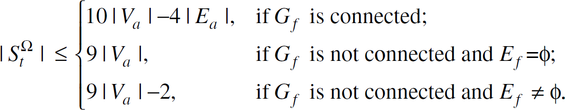
Theorem 5. An upper bound on the total number of FT nodes needed to achieve Ω-DOFT is given as

∣ S_{t}^{Ω} ∣\leq {\begin{cases} 10 ∣ V_{a} ∣ - 4 ∣ E_{a} ∣, & if G_{f} is connected; \\ 9 ∣ V_{a} ∣, & if G_{f} is not connected and E_{f} = ϕ; \\ 9 ∣ V_{a} ∣ - 2, & if G_{f} is not connected and E_{f} \neq ϕ . \end{cases}

(5)

4.2. Lower Bound on the Number of Fault Tolerance Nodes

To reduce energy consumption, it is desirable to minimize the number of FT nodes needed, i.e., to minimize the size of $S_{t}^{Ω}$ . In this section, we present a lower bound on the number of FT nodes needed to achieve the required Ω-DOFT (Ω  1) in wireless sensor networks. Let $N_{k}^{f} \subseteq N_{k}^{a}$ be the set of failing active neighbors of s_k, i.e., $S_{t}^{Ω} = ⋃_{s_{k} \in S_{a}} N_{k}^{Ω}$ . Let $N_{k}^{Ω} \subseteq N_{k}^{s}$ be the set of FT nodes for s_k, i.e., $S_{t}^{Ω} = ⋃_{s_{k} \in S_{a}} N_{k}^{Ω}$ .

We know from previous subsections that $\forall s_{k} \in S_{a}$ , FT nodes of s_k keep all neighbors nodes of s_k in N_k connected. This implies that the subgraph representing $N_{k}^{Ω}$ is a CDS of the subgraph representing N_k. When Ω = 1, the minimization of |S^Ω_t| is equivalent to finding the MCDS for the subgraph representing N_k for each active node s_k ∊ S_a. However, since no failing active node has any failing active neighbors for Ω = 1, such an MCDS for s_k also contains existing active neighbors in $N_{a}^{k}$ as existing dominating nodes. Let $S_{t}^{1}$ be the set of nodes selected as FT nodes to achieve 1-DOFT in the sensor network. It is then easy to see that a lower bound on the total number of FT nodes needed to achieve 1-DOFT, i.e., $| S_{t}^{1} |$ , is given by:

∣ S_{t}^{1} ∣ \geq {\begin{cases} 1, & if ∣ S_{a} ∣= 1; \\ 0, & if ∣ S_{a} ∣> 1. \end{cases}

(6)

Note that the best case of $∣ S_{t}^{1} ∣= 0$ when |S_a| > 1 rarely happens in practice, because it requires that neighbors of any active node are also neighbors of at least another active node. This implies that all nodes are within a circle of radius τ_c. Since |S_a| > 1, this makes the other |S_a| −1 nodes unnecessary. It is possible to have several such nodes but if |S_a| is very large, there will be a significant energy overhead for these nodes. When Ω > 1, the analysis is more complicated because when an active node s_k fails, some active neighbors in N^a_k may also fail at the same time.

To simplify the discussion, we define function $M$ as follows: ${\bar{S}}_{a} = M (S, S_{a})$ , where

$S_{a} \subseteq {\bar{S}}_{a}$

The subgraph representing ${\bar{S}}_{a}$ is a connected dominating set (CDS) of the graph representing S;

For all possible sets that satisfies 1) and 2), ͞S_a has the smallest size. We refer to determining ${\bar{S}}_{a}$ as a constrained minimum connected dominating set (constrained MCDS) problem. Note that if S_a = φ, then ${\bar{S}}_{a}$ is the MCDS of S. To achieve Ω-DOFT (Ω  1) in the wireless sensor network, we need to find the set of FT nodes $S_{t}^{Ω}$ such that $S_{t}^{Ω} = ⋃_{\forall S_{f} \subseteq S_{a}, ∣ S_{f} ∣\leq Ω} M (S ∖ S_{f}, S_{a} ∖ S_{f})$ . Let $N_{k}^{f} \subseteq N_{k}^{a}$ be the set of failing active neighbors of s_k. We can obtain a lower bound on the number of FT nodes needed to achieve Ω-DOFT (Ω > 1) as follows [32]:

\begin{aligned} | S_{t}^{Ω} | = | ⋃_{\forall | S_{f} ∣= Ω, S_{f} \subseteq S_{a}} ⋃_{s_{k} \in S_{f}} N_{k}^{Ω} | \geq | ⋃_{\forall | S_{f} | \leq Ω, S_{f} \subseteq S_{a}} (⋃_{\forall s_{k} \in S_{f}} M (N_{k} ∖ N_{k}^{f}, N_{k}^{a} ∖ N_{k}^{f})) | \\ \Rightarrow | S_{t}^{Ω} | \geq | ⋃_{\forall | S_{f} | \leq Ω, S_{f} \subseteq S_{a}} M (S ∖ S_{f}, S_{a} ∖ S_{f}) | \end{aligned}

(7)

Note that if $Ω =∣ S_{a} ∣, S_{a} ∖ S_{f} = ϕ$ , then $∣ S_{t}^{Ω} ∣\geq∣ M (S ∖ S_{a}, ϕ) ∣$ .

4.3. Connectivity-oriented Selection of Fault Tolerance Nodes

Since the CDS and MCDS problems are NP-complete [3,4,8,25,28], finding the constrained MCDS to achieve Ω-DOFT as shown in Equation (7) is also NP-complete. When only single-hop knowledge is available, for any s_k ∊ S_a, there are a total of $\sum_{i = 1}^{Ω} (\begin{matrix} ∣ N_{k}^{a} ∣ \\ i \end{matrix})$ possible combinations of failing nodes for s_k; as a result, the total number of possible combination of failing nodes for all the active nodes is $\sum_{\forall s_{k} \in S_{a}} (\sum_{i = 1}^{Ω} (\begin{matrix} ∣ N_{k}^{a} ∣ \\ i \end{matrix}))$ . Each evaluation requires the finding of the MCDS for neighbors of the failing node. Even though failing active nodes may share many neighbors, a through evaluation in this way is still computationally very expensive.

For a wireless sensor network with a set S_a of active nodes serving as a backbone, the maximum number of nodes that can fail is |S_a|. We propose the following distributed procedure to achieve fault tolerance for the simultaneous failure of up to |S_a|. The proposed distributed procedure is based on the algorithm from [28]. Note that other heuristics, such as the algorithms described in [3,25], can also be used as the base for building our distributed procedure, since the proposed fault tolerance procedure is a stand-alone module operating on the existing subset of backbone nodes. The procedure contains three steps as shown in Fig. 3 .

In Step 1 of Fig. 3, each active node selects a FT node for any of its disconnected active neighbors. We refer to this type of FT nodes as gateway FT nodes since they provide alternative routing paths for active neighbors of the failing node. When that potential failing node actually fails, the network traffic from the failing node to its active neighbors can still be delivered. Though the first type of FT nodes are able to take care of the routing data originating from failing active nodes, they are not necessarily connected among each other and are not necessarily connected to sleeping neighbors of the failing active node. Step 2 in Fig. 3 deals with this problem by using a modified version of the algorithm proposed in [28], which proposed a distributed approach for constructing the CDS for a connected but not a completely connected graph. In the worst case, when all nodes in S_a fail at the same time, the subgraph representing the FT nodes should be a CDS of the subgraph representing S_s. We can therefore utilize the algorithm proposed in [28] with the target graph representing S_s. Note that in Step 2, we have already found gateway FT nodes, therefore Step 2 needs only check for connectivity of disconnected FT nodes. To ensure that the proposed distributed procedure is also applicable to more general scenarios, Step 3 is added to handle the case that the subgraph representing S_s is a completely connected graph. Let Δ be the maximum node degree. In Fig. 3, Step 1 takes O(Δ³) time, Step 2 takes O(Δ²) time, and Step 3 takes O(Δ) time. Therefore, the proposed procedure takes O(Δ³) time. We next prove that the proposed distributed procedure achieves | S_a | -DOFT for a wireless sensor network with the set of active nodes given by S_a.

Figure 3

Distributed fault tolerance nodes selection procedure.

Theorem 6. Assume that all nodes in S are connected, i.e., ∀s_i, S_j ∊ S, there exists a routing path from s_i to s_j. Assume that S_a is the set of active nodes as a backbone that keeps all nodes connected. Assume that S_t is the set of FT nodes obtained from the distributed FT selection procedure given by Fig. 3 . The set S_t achieves Ω-DOFT in this wireless sensor network, where Ω = | S_a|.

Proof. Since the maximum number of nodes that can fail is | S_a|, we only need to consider the case that the selected FT nodes in S_t are able to keep the network fully connected when all nodes in S_a fail. Let G_s(V_s, E_s) be the subgraph representing S_s = S\S_a and G_t(V_t, E_t) be the subgraph representing S_t. To prove that G_t is a CDS of G_s, we first show that G_t is connected, then we show that for any ν ∊ V_s, ν is either in V_t or adjacent to a vertex in V_t.

Consider any u, ν ∊ V_t. Since G_s is connected, ∃P(u, ν) as the shortest path from u to ν in G_s, where P(u, ν) ⊆ V_s is the set of the vertices in the path. If | P(u, ν)| = 2, the theorem is trivially proved. Assume |P(u, ν)|  3, and let P(u, ν) = {u, u₁, u₂, …, ν}. Consider predecessor vertices of u in P(u, ν), i.e., u₁. Since u ∊ V_t, from Step 2 in Fig. 3, u₁ has to be in V_t, irrespective of whether u₂ is in V_t. The same argument holds for u₂. Doing this repeatedly, we have ∀w ∊ P(u, ν), w ∊ V_t, i.e., P(u, ν) ∊ V_t. Next, ∀ν ∊ V_s, from Step 3 in Fig. 3, ν has at least one FT neighbor. Therefore, G_t is a CDS of G_s.

5. Coverage-Centric Fault Tolerance

In Section 4, we have discussed the Ω-DOFT problem for fault-tolerant communication connectivity of up to Ω active nodes failing simultaneously (Ω > 1). However, we should also take fault tolerance for sensing coverage into account to achieve the surveillance goal over the field of interest. This implies that the nodes selected as FT nodes must be able to provide enough sensing coverage over the areas that were originally under the surveillance of the Ω failing active nodes.

5.1. Loss of Sensing Coverage from Failing Nodes

Recall the collective coverage probability for a grid point g_i defined in Section 3. Since only the active nodes in S_a perform communication and sensing tasks, the collective coverage probability for g_i is actually from nodes in $S_{i}^{a}$ , where $S_{i}^{a} \subseteq S_{i}$ is the set of active nodes that can detect g_i. When the nodes fail in the network, the set of active nodes that can detect g_i, i.e., $S_{i}^{a}$ , changes with time, which subsequently changes the sensing coverage over that grid point. Let q_i(S) be a mapping from a set S of nodes to the coverage probability for grid point $g_{i}, p_{i} (t)$ be a mapping from a time instant t to the coverage probability for grid point g_i, and S(t) be a mapping from a time instant t to a set of nodes. Then S_i(t) is the set of nodes that can detect grid point g_i at time instant t. For example, if at time instant t, only nodes in the subset $S_{i}^{a}$ , i.e., active nodes, detect grid point g_i, therefore $S_{i} (t) = S_{i}^{a}$ and $p_{i} (t) = q_{i} (S_{i} (t)) = q_{i} (S_{i}^{a})$ . Therefore, from Equation (2), the collective coverage probability of g_i under the fault tolerance constraint is a function of time given as follows:

p_{i} (t) = q_{i} (S_{i}^{a} (t)) = 1 - \prod_{s_{k} \in S_{i}^{a} (t)} (1 - p_{i}^{k}),

(8)

where $S_{i}^{a} (t)$ is the set of active nodes that can still detect g_i at time instant t. Therefore, the goal is to ensure that the selected FT nodes and existing active nodes, i.e., $S_{a}^{Ω} = S_{a} \cup S_{t}^{Ω}$ , are able to keep the sensor field adequately covered whenever up to Ω active nodes fail. Thus, successful sensing coverage over the sensor field for FTNS in wireless sensor networks is indicated by:

\forall g_{i} \in G, p_{i} (t) \geq p_{t h},

(9)

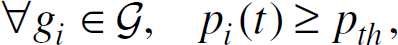
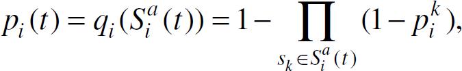
where p_th is the coverage probability threshold defined in Section 3. Theorem 7 shows the relationship between the loss of sensing coverage and the fault-tolerant operation in wireless sensor networks.

Theorem 7. Assume that all nodes in S are connected, i.e., $\forall s_{i}, s_{j} \in S$ , there exists a routing path from s_i to s_j. Let $G$ be the set of all the grid points in the sensor field. Let S_i be the set of nodes that can detect the grid point $g_{i} \in G$ initially after the deployment. Let S_i(t) be the set of nodes that can detect g_i at time t, and $S_{i}^{f} (t)$ be the set of failing active nodes for g_i at time t. Throughout the operational life time of a sensor network, $\forall g_{i} \in G$ , the following must be satisfied for any time instant t:

p_{f} (t + 1) \leq \frac{p_{i} (t) - p_{t h}}{1 - p_{t h}} .

(10)

where $p_{i} (t) = 1 - \prod_{s_{k} \in S_{i} (t)} (1 - p_{i}^{k})$ .

Proof. Consider time instants t and t + 1. Obviously we have $S_{i} (t) \subseteq S_{i}$ and $S_{i} (t) = S_{i} (t + 1) \cup S_{i} f (t + 1)$ . From Equation (8), we have

\begin{aligned} P_{i} (t) = 1 - \prod_{s_{k} \in S_{i} (t)} (1 - p_{i}^{k}) & = 1 - \prod_{s_{k} \in S_{i} (t + 1) \cup S_{i}^{f} (t + 1)} (1 - p_{i}^{k}) \\ = 1 - \prod_{s_{k} \in S_{i} (t + 1)} (1 - p_{i}^{k}) \prod_{s_{k} \in S_{i}^{f} (t + 1)} (1 - p_{i}^{k}) . \end{aligned}

Similarly, $p_{i} (t + 1) = 1 - \prod_{s_{k} \in S_{i} (t + 1)} (1 - p_{i}^{k})$ . Let $p_{f} (t) = 1 - \prod_{s_{k} \in S_{i}^{f} (t)} (1 - p_{i}^{k})$ and $p_{f} (t + 1) = 1 - \prod_{s_{k} \in S_{i}^{f} (t + 1)} (1 - p_{i}^{k})$ . Then we have

p_{i} (t) = 1 - (1 - p_{i} (t + 1)) (1 - p_{f} (t + 1)) = p_{f} (t + 1) + p_{i} (t + 1) (1 - p_{f} (t + 1)) .

Therefore, $p_{i} (t + 1) = \frac{p_{i} (t) - p_{f} (t + 1)}{1 - p_{f} (t + 1)}$ . From Equation (9), which expresses the FTNS sensing coverage condition for any time instant, we have $p_{i} (t + 1) \geq p_{t h} \Rightarrow \frac{p_{i} (t) - p_{f} (t + 1)}{1 - p_{f} (t + 1)} \geq p_{t h}$ , which implies that $p_{f} (t + 1) \leq \frac{p_{i} (t) - p_{t h}}{1 - p_{t h}}$ .

From the proof of Theorem 7, we see that $p_{f} (t + 1)$ represents the sensing coverage loss at time t + 1 at grid point g_i caused by the failing nodes in $S_{i}^{f} (t + 1)$ . To satisfy the coverage probability threshold requirement, $p_{f} (t + 1)$ must not exceed $\frac{p_{i} (t) - p_{t h}}{1 - p_{t h}}$ . In other words, if we can bound the coverage loss p_f(t) below $\frac{p_{i} (t) - p_{t h}}{1 - p_{t h}}$ during the operational lifetime of the sensor network for all grid points on the field, the sensor network is able to tolerate up to Ω nodes failing simultaneously. When p_i(t) drops, the bound on the coverage loss from failing nodes at the next time instant, i.e., p_f(t + 1), becomes tighter since $\frac{p_{i} (t) - p_{t h}}{1 - p_{t h}}$ decreases when p_i(t) decreases. This can also be used as a warning criteria to inform the base station whether a current node may lose sensing coverage over its sensing area.

Note that the fault tolerance problem for sensing coverage differs from the fault tolerance problem for communication connectivity discussed in Section 4 since there is no direct relationship between the number of failing nodes and the coverage loss p_f(t). For example, for g_i with |S_i(t)|= 1, p_i(t) might be the same as p_j(t) for g_i where |S_j(t)| = 1, 2, 3 or even higher. This is due to the fact that for any grid point g_i, p_i(t) is not directly related to the number of nodes that can detect g_i but rather to the distances from these nodes to g_i, as defined by Equation (1).

5.2. Distributed Approach

We next propose a coverage-centric fault tolerance algorithm that can be executed in a distributed manner, and requires much less computation than the centralized case. Without loss of generality, assume r_c  2r_s, i.e., S_i ⊆ N_k. For grid point g_i ∊ A_k corresponding to node $s_{k} \in S_{i}^{a} \subseteq S_{a}$ , the maximum coverage loss happens when all nodes in $S_{i}^{a}$ fail. In this case, the coverage loss for g_i, denoted as $q_{i} (S_{i}^{a})$ , is given as $q_{i} (S_{i}^{a}) = 1 - \prod_{s_{k} \in \cup S_{i}^{a}} (1 - p_{i}^{k})$ . Let $S_{i}^{Ω} \subseteq S_{i}^{s}$ be the set of FT nodes for grid point g_i. The coverage compensation from $S_{i}^{Ω}$ , denoted as $q_{i} (S_{i}^{Ω})$ , is given as $q_{i} (S_{i}^{Ω}) = 1 - \prod_{s_{k} \in S_{i} Ω} (1 - p_{i}^{k})$ . Let $q_{i} (S_{i}^{a} \cup S_{i}^{Ω})$ be the coverage from both active nodes and the FT nodes for g_i. Similarly, $q_{i} (S_{i}^{a} \cup S_{i}^{Ω}) = 1 - \prod_{s_{k} \in S_{i}^{a} \cup S_{i}^{Ω}} (1 - p_{i}^{k})$ . Assuming that the maximum coverage loss happens at time instant $t + 1, i . e ., S_{i} (t) = S_{i}^{a} \cup S_{i}^{Ω}, S_{i} (t + 1) = S_{i}^{Ω}$ , and $S_{f} (t + 1) = S_{i}^{a}$ , then accordingly, we have corresponding expression as $p_{i} (t) = q_{i} (S_{i}^{a} \cup S_{i}^{Ω}), p_{i} (t + 1) = q_{i} (S_{i}^{Ω})$ (1), and $p_{f} (t + 1) = q_{i} (S_{i}^{a})$ . From Equation (10), if the following is satisfied for all grid points in the sensing area of s_k, i.e., A_k, then the node s_k is able to tolerate the maximum number of failing active nodes within its own sensing area without losing sensing coverage:

p_{f} (t + 1) \leq \frac{p_{i} (t) - p_{t h}}{1 - p_{t h}} \Rightarrow q_{i} (S_{i}^{a}) \leq \frac{q_{i} (S_{i}^{a} \cup S_{i}^{Ω}) - p_{t h}}{1 - p_{t h}}, \forall g_{i} \in A_{k} .

(11)

Equation (11) requires $\sum_{j = 1}^{| S_{i}^{s} |} (\begin{matrix} ∣ S_{i}^{s} ∣ \\ j \end{matrix})$ evaluations for a total of |A_k| grid points within s_k&s sensing area. When each active node executes the evaluation procedure described by Equation (11), the maximum total number of evaluations is $\sum_{g_{i} \in G} \sum_{j = 1}^{∣ S_{i}^{s} ∣} (\begin{matrix} ∣ S_{i}^{s} ∣ \\ j \end{matrix})$ . However, note that $q_{i} (S_{i}^{a} \cup S_{i}^{Ω}) = q_{i} (S_{i}^{a}) + q_{i} (S_{i}^{Ω}) - q_{i} (S_{i}^{Ω}) q_{i} (S_{i}^{Ω})$ , therefore, from Equation (11), we have

q_{i} (S_{i}^{a}) \leq \frac{q_{i} (S_{i}^{a} \cup S_{i}^{Ω}) - p_{t h}}{1 - p_{t h}} \Rightarrow q_{i} (S_{i}^{Ω}) \geq p_{t h},

(12)

which corresponds to the analysis in Theorem 7. Equation (12) implies that we can design the fault-tolerance nodes selection for sensing coverage in a much less computationally expensive way. Figure 4 shows the pseudocode for the coverage-centric fault tolerance node selection algorithm.

As shown in Fig. 4, to select the minimum number of FT nodes without a thorough evaluation over all subsets of nodes in $S_{i}^{s}$ , we first construct L_i from $S_{i}^{s}$ , where L_i is a list corresponding to the set of nodes $S_{i}^{s}$ such that L_i is constructed as a sorted list in the descending order of the individual coverage on grid point g_i of all nodes in $S_{i}^{s}$ . For any $s_{k} \in S_{i}^{s}$ , the corresponding element in L_i is denoted by l(s_k), which gives the position of s_k in the list L_i. Therefore, for any two different nodes $s_{k_{1}}, s_{k_{2}} \in S_{i}^{s}, l (s_{k_{1}}) \leq l (s_{k_{2}})$ if $p_{i}^{k_{1}} \geq p_{i}^{k_{2}}$ . We denote the length of the list L_i as |L_i|, where $∣ L_{i} ∣=∣ S_{i}^{s} ∣$ . We define the position l(s_k) as a positive integer, where l(s_k) = 1 if s_k is the first element in L_i and l(s_k) = |L_i| if s_k is the last element in L_i. We refer to a subset containing a single node s_k in L_i at the j-th position by L_i(j), i.e., L_i(j) = {s_k|l(s_k) = j, 1  j  |L_i|}. Furthermore, we use L_i(j₁, j₂,…,j_u) to denote the subset of nodes ${s_{k_{1}}, s_{k_{2}}, \dots, s_{k_{u}} ∣ l (s_{k_{1}}) = j_{i}, l (s_{k_{2}}) = j_{2}, \dots, l (s_{k_{u}}) = j_{1}$ and $1 \leq j_{1} \leq j_{2} \leq \dots \leq j_{u} \leq∣ L_{i} ∣}$ . Thus, for a given grid point g_i, when there are enough nodes in $S_{i}^{s}$ for g_i as FT nodes, Fig. 4 is able to generate the subset of FT nodes from $S_{i}^{s}$ with the minimum number of FT nodes among for g_i. Note however that to avoid the repeated selection of the same nodes for different grid points, before selecting the FT nodes for the current grid point, the coverage support from existing FT nodes in $S_{i}^{Ω}$ is checked first to see if they already provide enough coverage support when active nodes fail; see line 3 in Fig. 4 . Therefore, even though the number of FT nodes selected is locally minimum for a given grid point, it is not necessarily a global minimum.

Figure 4

Pseudocode for the distributed coverage-centric fault tolerance nodes selection.

Note that the evaluation procedure is per grid point, which can be executed on either a sleeping node or an active node. For any $g_{i} \in G$ , only one node needs to perform the selection of FT nodes for g_i. This implies that the total number of nodes required for executing such evaluation procedure is $⌈ \frac{∣ G ∣}{∣ A_{k} ∣} ⌉$ or $⌈ \frac{A}{π r_{s}^{2}} ⌉$ where A is the area of the surveillance field (assuming that either $r_{c} \geq 2 r_{s}$ or $⌈ \frac{2 r_{s}}{r_{c}} ⌉$ -hop knowledge is available). Also note that in Fig. 4, there is no need to calculate $q_{i} (S_{i}^{a})$ every time since it is available from the previous stage when S_a is determined. Further computation can be reduced by temporarily storing the $q_{i} (S_{i}^{Ω})$ for the current grid point for evaluation at the next grid point, where $q_{i} (S_{i}^{Ω} \cup S_{k}^{Ω})$ can be obtained as: $q_{i} (S_{i}^{Ω} \cup S_{k}^{Ω}) = q_{i} (S_{i}^{Ω}) + q_{i} (S_{k}^{Ω}) - q_{i} (S_{i}^{Ω}) q_{i} (S_{k}^{Ω})$ .

The sorting procedure needed to construct L_i from $S_{i}^{s}$ has a time complexity of O(Δ log Δ), where Δ is the maximum node degree. The pseudocode between line 5 to line 9 in Fig. 4 for FT nodes selection has a time complexity of O(Δ). Since the distributed coverage-centric fault-tolerant procedure in Fig. 4 is carried out per grid point, the overall time complexity for the distributed coverage-centric fault-tolerant node selection has a time complexity as $O (m Δ (1 + log Δ)) = O (m Δ log Δ)$ , where m is the number of grid points. The next theorem shows that the procedure of Fig. 4 leads to the smallest number of FT nodes needed to satisfy the coverage threshold for a given grid point g_i. The proof is given in the appendix.

Theorem 8. For a grid point g_i, the distributed coverage-centric fault-tolerance node selection procedure given by the pseudocode in Fig. 4 gives the minimum number of fault-tolerance node.

As shown in Figs. 3 and 4, the proposed scheme does not require a centralized server to determine backup nodes for the existing backbone. FT nodes are designated in a distributed fashion; this procedure requires only localized communication (single-hop or restricted hop communication between nodes). The proposed self-organization approach for fault tolerance is therefore scalable, which makes it suitable for ad hoc sensor networks with a large number of deployed nodes.

6. Simulation and Discussion

We have implemented CCANS in ns2 and integrated as a module in the ESP AESOP protocol. The Emergent Surveillance Plexus (ESP) [34] is a Multi-disciplinary University Research Initiative (MURI), whose goal is to advance the surveillance capabilities of wireless sensor networks. It involves participants from Pennsylvania State University, University of California at Los Angles, Duke University, University of Wisconsin, Cornell University, and Louisiana State University. AESOP stands for An Emergent-Surveillance-Plexus Self-Organizing Protocol, which is designed for target tracking in wireless sensor networks with high tracking quality and energy efficiency [5]. A more detailed description of the AESOP protocol can be found in [5].

6.1. Simulation Results

In a simulation for the proposed fault-tolerant self-organization algorithms, we first collect the data from the distributed CCANS procedure described in Section 3. We next evaluate the proposed distributed FTNS procedure using MatLab by feeding the data collected from CCANS as inputs. The data from CCANS contains locations of sensor nodes after deployment and their final state decisions. There are 150, 200, 250, 300, 350, and 400 nodes in each random deployment, respectively, on a 50 × 50 grid representing a 50m × 50m sensor field. All nodes have the same maximum communication radius r_c = 20m and maximum sensing range r_s = 10m. The value of Ω is set to the number of active nodes. Figures 5–8 show the simulation results for distributed fault-tolerance self-organization procedure.

Figure 5(b)(i) shows the results obtained for connectivity-oriented selection of FT nodes. Note that the percentage of FT nodes decreases nearly at the same rate as the percentage of active nodes. This is because the connectivity-oriented FT nodes selection algorithm is executed in a distributed manner and each node uses only one-hop knowledge. Note also that the percentage of FT nodes is lower than the percentage of active nodes determined by CCANS. This is because CCANS considers both communication connectivity and sensing coverage in selecting active nodes. Figure 5(b)(ii) shows the results for coverage-centric selection of FT nodes. Since the coverage-centric fault-tolerance nodes selection procedure given by Fig. 4 has been proven to generate the minimum number of fault-tolerance nodes, the percentage shown in Fig. 5 (b)(ii) is much lower than the percentage of active nodes from CCANS.

The distributed fault-tolerance nodes selection procedure contains two stages. We consider two cases for the implementation, namely “FTNS-1” and “FTNS-2”. FTNS-1 refers to the case that the first stage is the coverage-centric selection of fault-tolerance nodes (FTNS-1 Stage 1) and the second stage is the connectivity-centric selection of FT nodes (FTNS-1 Stage 2). FTNS-2 refers to the case that the first stage is the connectivity-centric selection of FT nodes (FTNS-2 Stage 1) and the second stage is the coverage-centric selection of FT nodes (FTNS-2 Stage 2). Figure 5(a) presents the result for the distributed FTNS algorithm. In both FTNS-1 and FTNS-2, the FT nodes that have already been selected in Stage 1 are checked first in Stage 2 to see if they already provide enough sensing coverage for fault tolerance. This decreases the number of FT nodes needed for Stage 2 of coverage-centric FT nodes selection, which is shown in Fig. 5 (a). Note that in Fig. 5 (a)(ii), the percentage of FT nodes in Stage 1 is the same as the percentage of FT nodes at the end of the FTNS procedure. This is due to the fact that we have r_c = 2r_s in this scenario. As shown in [31], when r_c = 2r_s, the connectivity is automatically guaranteed by the subset of nodes needed to maintain the sensing coverage.

Figure 5

Simulation results: (a) Percentage of FT nodes: (i) FT nodes for connectivity only; (ii) FT nodes for coverage only. (b) Percentage of FT nodes for the distributed FTNS procedure (with both coverage and connectivity concerns): (i) FTNS-1: Stage 1 selects FT nodes for coverage and FTNS Stage 2 selects FT nodes for connectivity; (ii) FTNS-2 Stage 1 selects FT nodes for connectivity and FTNS Stage 2 selects FT nodes for coverage.

Figure 6

Simulation results: (a) Effect of failing active nodes vs. activated FT nodes for FTNS-1: (i) Average coverage loss from failing active nodes; (ii) Average number of activated FT nodes; (iii) Average coverage loss from failing active nodes; (iv) Average number of activated FT nodes; (b) Effect of failing active nodes vs. activated FT nodes for FTNS-2: (i) Average coverage loss from failing active nodes; (ii) Average number of activated FT nodes; (iii) Average coverage loss from failing active nodes; (iv) Average number of activated FT nodes.

Figure 7

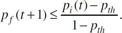
Average grid point coverage when active nodes fail during the simulation.

Next, we simulate the failing of active nodes to show that FT nodes are able to provide the coverage and connectivity when active nodes fail. This is shown in Fig. 6 . The sensor network layout and configuration are the same as those in Fig. 5 . We use a simplified model for generating the failing active nodes. For a total simulation time of 200 minutes, we select a random number of active nodes from the currently alive active nodes every 10 minutes, and assign them as failing nodes. The neighboring FT nodes determine that these nodes have failed. As shown in Fig. 6, the failing of active nodes leads to an activation of the designated FT neighbors. The loss of coverage from the failing active nodes are compensated by the coverage support from the activated FT nodes. The simulation stops when all active nodes have failed. Fig. 7 shows the change in coverage probability for grid points in the sensor field. Note that the average grid point coverage probability decreases with time. This is due to the fact that the coverage-centric FT nodes selection only selects the minimum number of FT nodes to save energy; the goal is not to maximize the coverage. However, at any time instant, the coverage probability is always higher than the required coverage probability threshold p_th = 0.8. Also note that at any time instant, the connectivity is guaranteed by the activated FT nodes and alive active nodes for both FTNS-1 and FTNS-2.

Figure 8

Communication data message size in FTNS for FT nodes selection.

6.2. Discussion

Note that upper bounds on the number of the fault-tolerance node given in previous sections are important because they can be used as a guideline for the initial sensor nodes deployment to achieve fault-tolerant self-organization. For example, as shown by Fig. 5, we can deploy the number of sensor nodes that are sufficient enough to provide the required level of fault tolerance in the sensor network. The lower bound on the number of fault-tolerance node is useful since it can be used as a baseline for comparing different heuristics. Note that the problem of finding a minimum connected dominating set (MCDS) for a general graph is a NP -complete and it is hard to approximate. The original work of using MCDS as a backbone for routing by Bharghavan and Das in [4] has a approximation ratio of 3H(Δ), where Δ is the maximum node degree and H(Δ) is the Δth Harmonic number given $H (Δ) = \sum_{i = 1}^{Δ} \frac{1}{i}$ . A comparison of recent distributed algorithms for forming CDS described in [3,25,28] can be found in [3]. In this paper, we used the distributed algorithm proposed in [28] for its simplicity of implementation. However, the proposed fault-tolerance procedure in this paper is not limited by any particular heuristics for backbone nodes selection to form CDS. In our case, the lower bound is not on the set of all nodes but the subset of nodes that are not selected as backbone nodes, i.e., candidate fault-tolerance nodes. This is referred to as the constrained minimum connected dominating set problem in our paper. Therefore, heuristics in existing literatures such as [3,4,25,28] can be directly used to obtain the approximations of MCDS by only applying it on the subset of non-backbone nodes.

The proposed distributed fault-tolerance nodes selection procedure is a localized algorithm. Localized algorithms are considered as a special type of distributed algorithms where only a subset of nodes in the wireless sensor networks participate in sensing, communication, and computation [18]. For either stage in the proposed distributed fault-tolerance nodes selection procedure, it requires only local knowledge and constant rounds of communication for message exchange among the neighborhood. From the discussion in Subsection 4.3 and 5.2, the total time complexity for the distributed FTNS is O(mΔ LoGΔ + Δ³). For message complexity, both stages in FTNS require the exchange of a constant number of messages within the neighborhood. The active nodes in the backbone first carries out the computation for connectivity checking and coverage evaluation to select a subset of nodes from its sleeping neighbors, then it broadcasts the list of selected FT neighbors within its neighborhood. The designated FT nodes need not be activated until the active nodes fail. In Fig. 8, we show the evaluation of communication data size for FT nodes selection.

In FT nodes selection, active nodes send the message containing the list of node ids of the designated FT neighbors. Neighbors of active nodes search the received id list and set themselves as FT nodes for that active node, i.e., FT nodes that can be activated into an active state by their failing active neighbors. The designated FT nodes then send an acknowledge message back to the active nodes to confirm the FT node assignment. Assuming that there is no packet loss, this takes 2 rounds of communication within the neighborhood of active odes. The message size complexity is then O(Δ). For the activation of FT nodes, we assume that designated FT nodes periodically poll their active neighbors about whether they are still alive or not. The polling frequency depends on the sensor network application requirement and sensor nodes failure distribution, since it should not require excessive energy and bandwidth. The problem of determining the polling frequency is not considered in this paper. Note that it is possible to simply let all sleeping nodes do the polling without designating any fault-tolerance nodes. However, this also means that when an active node fails, all its sleeping neighbors have to become active. This adversely affects the potential of extending the lifetime for the densely deployed sensor network. Figure 8 shows the average communication data size for both FTNS-1 and FTNS-2.

7. Conclusions

In this paper, we have investigated fault tolerance for coverage and connectivity in wireless sensor networks. Fault tolerance is necessary to ensure robust operation for surveillance and monitoring applications. Since wireless sensor networks are made up of inexpensive nodes and they operate in harsh environments, the likely possibility of node failures must be considered. We have characterized the amount of redundancy required in the network for fault tolerance. Based on an analysis of the redundancy necessary to maintain communication connectivity and sensing coverage, we have proposed the distributed FTNS algorithm for fault-tolerant self-organization. FTNS is able to provide a high degree of fault tolerance such that even when all of these active nodes fail simultaneously, the coverage and the connectivity in the network are not affected. The proposed distributed FTNS approach is scalable and requires only localized communication. We have implemented FTNS in MatLab and presented representative simulation results.

Footnotes

Appendix

References

Agre

J. R.

Clare

L. P.

, “An integrated architecture for cooperative sensing networks,” IEEE Computer Magazine, vol. 33, no. 5, pp. 106–108, 2000.

Akyildiz

I. F.

Sankarasubramaniam

Cayirci

, “A survey on sensor networks,” IEEE Communications Magazine vol. 40, no. 8, pp. 102–114, 2002.

Alzoubi

K. M.

Wan

P. J.

Frieder

, “Distributed heuristics for connected dominating sets in wireless ad hoc networks,” J. Communications and Networks vol. 4, no. 1, pp. 1–8, 2002.

Bharghavan

Das

, “Routing in ad hoc networks using minimum connected dominating sets,” Proc. IEEE ICC, pp. 376–380, 1997.

Biswas

Phoha

, “A Sensor network test-bed for an integrated target surveillance experiment,” Proc. IEEE Conf. Local Computer Networks, pp. 552–553, 2004.

Chessa

Santi

, “Crash faults identification in wireless sensor networks,” Computer Communications vol. 25, no. 14, pp. 1273–1282, 2002.

Estrin

Girod

Pottie

Srivastava

, “Instrumenting the world with wireless sensor networks,” Proc. Intl. Conf. Acoustics, Speech, and Signal Processing vol. 4, pp. 2033–2036,2001.

Garey

M. R.

Johnson

D. S.

, Computers and Intractability: A guide to the theory of NP-completeness, W. H. Freeman and Co., 1979.

Iyengar

S. S.

Sharma

M. B.

Kashyap

R. L.

, “Information routing and reliability issues in distributed sensor networks,” IEEE Trans. Signal Processing vol. 40, no. 2, pp. 3012–3021, 1992.

10.

Koushanfar

Potkonjak

Sangiovanni-Vincentelli

, “Fault tolerance in wireless ad-hoc sensor networks,” Proc. IEEE Sensors, 2002.

11.

Krasniewski

Varadharajan

Rabeler

Bagchi

Y. C.

, “TIBFIT: Trust Index Based Fault Tolerance for Arbitrary Data Faults in Sensor Networks,” Proc. Intl. Conf. Dependable Systems and Networks (DSN), 2005.

12.

Krishnamachari

Iyengar

S. S.

, “Distributed Bayesian algorithms for fault-tolerant event region detection in wireless sensor networks,” IEEE Trans. Computers vol. 53, pp. 241–250,March 2004.

13.

Gui

Mohapatra

, “Power conservation and quality of surveillance in target tracking sensor networks,” Proc. ACM/IEEE MobiCom, pp. 129–143, 2004.

14.

Gupta

Das

S. R.

Quinyi

, “Connected sensor cover: self-organiziation of sensor networks for efficient query execution,” Proc. IEEE/ACM MobiHoc, pp. 189–200, 2003.

15.

X. Y.

Wan

P. J.

Wang

C. W.

, “Fault tolerant deployment and topology control in wireless networks,” Proc. ACM/IEEE MobiHoc, pp. 117–128, 2003.

16.

Lindsey

Raghavendra

C. S.

, “PEGASIS: power-efficient gathering in sensor information systems,” Proc. IEEE Aerospace Conf. vol. 3, pp. 1125–1130,2002.

17.

Marzullo

, “Implementing fault-tolerant sensors,” Technical Report 89–997, Computer Science Department, Cornell University, 1989.

18.

Meguerdichian

Slijepcevic

Karayan

Potkonjak

, “Localized algorithms in wireless ad-hoc networks: location discovery and sensor exposure,” Proc. MobiHoc, pp. 106–116, 2001.

19.

Olariu

Zomaya

A. Y.

, “An overview of mobile communications and computing,” in State of the Art Series, Abdallah

A. E.

(Ed), Heidelberg: Springer Verlag, 2004.

20.

Polastre

Hill

Culler

, “Versatile low power media access for wireless sensor networks,” Proc. ACM SenSys, pp. 95–107, 2004.

21.

Prasad

Iyengar

S. S.

Rao

R. L.

Kashyap

R. L.

, “Fault- tolerant sensor integration using multiresolution decomposition,” Physical Rev. E vol. 49, no. 4, 1994.

22.

Schwiebert

Gupta

S. D. S.

Weinmann

, “Research challenges in wireless networks of biomedical sensors,” Proc. ACM/IEEE MobiCom, pp. 151–165, 2001.

23.

Seada

Zuniga

Helmy

Krishnamachari

. “Energy-efficient forwarding strategies for geographic routing in lossy wireless sensor networks,” Proc. ACM SenSys, pp. 108–121, 2004.

24.

Siewiorek

D. P.

Swarz

R. S.

, Reliable Computer Systems: Design and Evaluation, MA: A. K. Peters, 1998.

25.

Stojmenovic

Seddigh

Zunic

, “Dominating sets and neighbor elimination based broad-casting algorithms in wireless networks,” Proc. IEEE Conf. System Sciences 13(1), pp. 14–15, 2002.

26.

Wang

Heinzelman

W. B.

Chandrakasan

A. P.

, “Energy-scalable protocols for battery-operated micro sensor networks,” IEEE Workshop on Signal Processing Systems, pp. 483–490, 1999.

27.

Wang

X. R.

Xing

G. L.

Zhang

Y. F.

C. Y.

Pless

Gill

, “Integrated coverage and connectivity configuration in wireless sensor networks,” Proc Proc. ACM SenSys, pp. 28–39, 2003.

28.

, “Extended dominating-set-based routing in ad hoc wireless networks with unidirectional links,” IEEE Transactions on Parallel and Distributed Computing vol. 22, 1–4, pp. 327–340, 2002.

29.

Heidemann

Estrin

, “Geography-informed energy conservation for ad hoc routing,” Proc. ACM/IEEE MobiCom COnference, pp. 70–84, 2001.

30.

Xue

Kumar

P. R.

, “The number of neighbors needed for connectivity of wireless networks,” Wireless Networks vol. 10, no. 2, pp. 169–181, 2004.

31.

Zou

Chakrabarty

, “A distributed coverage- and connectivity-centric technique for selecting active nodes in wireless sensor networks,” IEEE Trans. Computers vol. 54, pp. 978–991,August 2005.

32.

Zou

Chakrabarty

, “Fault-tolerant Self-Organization in Wireless Sensor Networks,” Proc. IEEE DCOSS/Lecture Notes in Computer Science LNCS 3560, pp. 191–205, Springer, New York, 2005.

33.

Crossbow Technology, http://www.xbow.com/Products/products.htm, page accessed on April 20, 2006.

34.

Emergent Surveillance Plexus (ESP): A multidisciplinary university research initiative (MURI), http://strange.arl.psu.edu/ESP, page accessed on April 20, 2006.

Redundancy Analysis and a Distributed Self-Organization Protocol for Fault-Tolerant Wireless Sensor Networks ∗

Abstract

Keywords

1. Introduction

2. Related Work

3. Preliminaries

3.1. Assumptions

3.3. Token-based CCANS Protocol

4.1. An Upper Bound on the Number of Fault Tolerance Nodes

5.1. Loss of Sensing Coverage from Failing Nodes

6.1. Simulation Results

7. Conclusions

Footnotes

Appendix

References