
Abstract
Wireless sensor nodes can be mobile within a chosen area and communicate with neighboring nodes in the bounds of protocol limits. Since communications among all network components in sensor networks are wireless, a peer-to-peer protocol is employed between two nodes. Among many concerns about design of sensor networks are growing bandwidth demands, speed of information retrieval, and transporting bytes over the wireless networks to provide a quality service for the diverse requirements of the users, such as signal processing or multimedia applications. Although traditional routing protocols ignore power management issues for sensor networks, design and implementation of an efficient energy based routing is in the core interest. In this paper, we discuss the current power management protocols, and propose an energy restrained information dissemination scheme. Experimental analysis and comparison with related work show that using the proposed scheme we can save substantial energy as compared to the prior methods.
Introduction
Within a wireless sensor network cloud, the sensor nodes may be installed in remote areas where repairing and replenishing the nodes may be impossible. The life span of the sensor node deeply depends on its battery lifetime. In order to prolong the sensor network lifetime, minimum battery power of the sensor nodes should be consumed. A considerable change in the topology of the sensor network may take place with each failing node, which requires re-organizing and re-routing the information [1]. Spatially distributed sensor nodes are densely deployed over a desired application area; the nodes are virtually connected by radio frequency, infrared, or other mediums without any physical wire connection. An event is detected by the sensor node, and the data collected by a sensor node traverses among other nodes in a wireless medium. The data from sensor nodes is gathered by a sink node, which acts like a base station. There may be multiple sinks in one wireless sensor network. The sink usually is robust in terms of processing speed, memory size, and battery capacity than other sensor nodes. The sink can be connected to the outside world through the Internet or satellite so that an end user can have access to the collected sensed data. Wireless sensor networks are made of nodes that have a processor, memory, wireless transceivers, sensor(s), location finding unit, and an onboard battery (Fig. 1). A radio transceiver is the leading energy consumer. In order to follow the economics of power savings, information transfer should not occur over a long distance and the node(s) should have the ability to switch between sleep and active modes.

Sensor node components.
In this paper we address a power management routing scheme appropriate for wireless sensor
networks that focuses on the dissemination of information from source to the sink. We achieve this
scheme by: Restricting minimum transmission around the sink and Setting up a battery threshold value.
We minimize transmission between the sink and its one-hop neighbors to enhance the economies of energy, and to apply a battery threshold value so that the probability of information packets being dropped decreases significantly. There are several benefits in doing so. First, the one-hop neighboring node(s) to the sink can transmit the information directly to the sink instead of broadcasting. Second, it ensures the graceful degradation of the network in a low-energy network, thereby enhancing the fault tolerance of the system. The remainder of the paper is organized as follows. Section 2 discusses related prior research and the specifics of power management. Sections 3 and 4 explain the proposed power management scheme and analyze the experimental results, formulating the base for future work.
Due to the nature of the applications supported by the sensor networks, such as a range of
estimations measuring temperature, pressure, humidity, seismic, thermal, acoustic, radar, noise
levels, etc., the sensor nodes need to be densely deployed in a magnitude much greater than
conventional ad hoc networks [1, 18]. All sensor nodes in a network are broadly
divided into different divisions or subsets, each of which provides a blueprint of vital sensing.
Different divisions take turns to being repeatedly switched on and off depending on a specific duty
cycle. Thus, the remaining nodes in a dormant subset will remain asleep until the next desired
action is chosen and the pattern is shifted. It is crucial to accurately estimate the availability
of power for a chosen time interval. Nodes can be switched on and off by choosing a specific duty
cycle and a random phase difference. But for a specific application, such as defense, there is a
trade off between utilization of battery life and capturing crucial information [2, 3]. Since a sensor network has limited bandwidth, it is
necessary to minimize communication between sensor nodes. In terms of power consumption, operation
of a wireless sensor node can be divided into three parts: sensing, processing, and transmission.
Among those three operations, it is known that the most power consuming task is data transmission.
Approximately 80% of power consumed in each sensor node is used for data transmission.
Energy-aware routing algorithms [4–6] discuss reducing the consumption battery-power at the
different nodes. Another concern is the narrow computing power of the sensor nodes and the limited
bandwidth [7] of the connecting nodes
that deter the communication of sensor nodes within the wireless sensor cloud. [8] discusses the energy management at the
MAC-medium access control layer in a wireless sensor network by using time division multiple access
along with periodic listen and sleep to avoid energy wastage. Power management techniques in
wireless sensor networks can be broadly classified as: Static power management broadly applied at the (node) design time, aiming at different levels of
system's hardware and software components, and Dynamic power management, applied at runtime. Dynamic power management takes into consideration
the runtime events, to reduce power when the sensor nodes are idle or catering to trivial
workloads.
Schemes such as auto shutdown and dynamic voltage scaling (DVS) have emerged as powerful methods for power-aware computing. In sensor networks, DVS plays an integral part in reducing the power consumed by a processor at each node during an active state. In a sensor node, the workload for a processor is not always constant; it varies over time [9]. Depending on the application involved and the processing speed, a node is either active or idle. This power optimization is realized by distributing workloads throughout an entire cycle of a processor. In other words, DVS minimizes the workload at a peak and spreads it during the idle times. Processor workload distribution can be accomplished by reducing processor frequency and voltage, which decreases the processing speed. One important point in designing a DVS system is that the processing speed has to be reduced without harming the efficiency of the entire network. Reducing only the frequency does not increase the processor power efficiency. By reducing the frequency, the power consumption is decreased, but the amount of task processed is also reduced. Because of the linear relationship between power consumption and task processing, the energy consumed by the task does not change. On the other hand, reducing the voltage applied to a processor by reducing the processing frequency leads to a quadratic energy reduction [9]. Therefore, by changing the frequency and the voltage, the total power consumed per task can be reduced. One aspect of DVS is predicting future workloads. Since decisions to spread workload are based on the current and future workloads, the accuracy of future workload estimation can dramatically change the efficiency of DVS. Thus, it is crucial to develop a good algorithm for predicting future workloads of nodes. Energy conservation is uniquely vital for embedded systems, such as obscured wireless sensors, which are deployed in applications where it is difficult to physically access sensors. Since the amount of power available to these systems is limited, it is considered a daunting challenge to minimize the energy consumption in order to broaden the life of the battery. In this section, we discuss the related power efficient routing schemes.
Low Energy Adaptive Clustering Hierarchy is an energy conserving communication protocol [13] where all the nodes in the network are uniform and energy constrained. An end user can access the remotely monitored operation where large numbers of nodes are involved. The nodes organize themselves into local clusters, with one node acting as the randomly selected local cluster-head. If the allocated cluster-heads are always fixed they would die quickly, ending the useful lifetime of all nodes belonging to those clusters. LEACH includes random alternation of the high-energy cluster-head nodes to enable the sensors to uniformly sustain the power. Sensors nominate themselves to be local cluster-heads at any given time with some probability. These cluster head nodes relay their status to the other sensors in the network. Each sensor node resolves what cluster to follow by choosing the cluster-head that requires the minimum communication energy. This allows the transceiver of each unassigned node to be turned off at all times except during its transmit time, thus minimizing the energy dissipated in each sensor. In Power-Efficient Gathering in Sensor Information Systems (PEGASIS) [14], each sensor node forms a pattern so that each node will receive from and transmit to a close neighbor. Each node takes turns being the leader for transmission to the base station so that the average energy spent by each node per round is reduced. PEGASIS outdoes LEACH'S performance by (1) purging the overhead of dynamic cluster formation, (2) decreasing the distance non leader-nodes must transmit, (3) reducing the number of transmissions among all nodes, and (4) using only one transmission to the base station per round.
Minimum Total Transmission Power Routing (MTTPR) [10]
This protocol is an on-demand, reactive routing scheme that seeks an optimal path from a source
to a destination node in mobile ad hoc networks only when such a path is needed. The objective of
MTPR development was to design an algorithm for finding a minimum transmission power consumption
path from a source to a destination in a power-constrained network. The basic idea is that if a
shortest path between two nodes is employed to transmit a data packet, the power consumed by the
transmission will be minimized because radio transmission power is proportional to the distance.
More specifically, the power consumed is directly proportional to dn, where d is the
distance between the two nodes and the value of n depends on d; namely n = 2 for short
distances and n = 4 for long distance [11]. Since data packets in ad hoc networks are transmitted in a multihop manner, the total
power required in transmitting between a source and a destination is the sum of the transmission
power consumed by each hop between two nodes necessary for a packet to reach the destination node.
Therefore, the total transmission power Pt, can be expressed as follows:

where D is the total number of nodes in the route, and n0 and nD are the source and destination nodes respectively [3]. An optimal route is determined by minimizing the total transmission power Pt over all possible routes between a source and destination node. This can be achieved by applying a shortest path algorithm, such as Dijkstra's algorithm. Because the value of n in dn is determined by the distance between the two nodes, MTTPR protocol tends to select routes that have more nodes, but with shorter distances for each hop. By selecting a path between a source and destination node with many short-distance hops, the total transmission power efficiency will be optimal. However, another consideration of the MTTPR is propagation delay. Because of the MTTPR route selecting method and the proportionality of transmission power to the distance, more nodes are usually involved in delivering data packets. Since each node requires some processing time, each node contributes to the propagation delay. Therefore, the more nodes in the route, the longer the propagation delay. Furthermore, each node consumes power in processing data packets. To address this problem, the receiving power of a node was introduced in addition to the transmission power [10]. By considering both power consumption factors, propagation delay and the number of nodes included in an optimal path can be reduced. Other consideration of the MTTPR protocol is the energy state of each node. Once an optimal path is selected, it can be used to transmit data packets as long as the route remains connected. Since some nodes can consume all of their energy while other nodes consume very little, patches can become disconnected and the network can become fragmented.
This scheme [10] is also an on-demand
reactive routing scheme. It selects an optimal data path based on the power remaining in each node.
To measure how much a node is willing to transmit a data packet at any given time,
‘t’, one proposed equation is

where

Hence, an optimal route in the MMBCR protocol is determined by finding a route having a minimum
Rj value over the set A of all the possible routes j ∈ A between two nodes

The MMBCR protocol is guaranteed to select a path whose minimum power capacity node is a maximum. However, unlike the MTTPR protocol, MMBCR does not take into account the total transmission energy consumed by each data packet transmission. Therefore, the path selected by MMBCR is not necessarily the most energy efficient path.
This protocol [10] is a routing scheme, which combines MTPR and MMBCR in an effort to maximize network power efficiency. CMMCR considers the best possible routing in terms of total transmission power and power consumption fairness over all routes in a network. In CMMBCR, the battery capacities of a node are divided into two states according to a threshold capacity value. There are three possible scenarios: (i) all nodes have capacities above the threshold (ii) all nodes have capacities below the threshold and (iii) some capacities are above and some are below the threshold. If the battery capacities of all nodes are above the threshold value, MTPR is used and CMMBCR selects a route with minimum total transmission power consumed per packet. Consequently, the power consumption of the whole network is minimized. On the other hand, if the battery capacities of all nodes are less than the threshold value, MMBCR is used, so that the lifetime of nodes with low capacity can be extended. In the third case, if there exists a route between a source and a destination for which all nodes have capacities above the threshold value, the optimal route is selected by applying MTPR. If all possible routes from a source to a destination contain only nodes with capacities below the threshold value, a route is selected by applying MMBCR. One disadvantage of CMMBCR is that it does not allocate energy utilization evenly throughout all nodes, as was expected [12]. Since the CMMBCR scheme is also a reactive routing scheme, a routing process is activated only when a route is needed for transmitting data packets. The power status of each node is not monitored continuously unlike proactive routing schemes that maintain routes periodically. Thus, after an optimal route is selected and as long as it is used for transmitting data packets, the power status of all nodes on the route is not monitored. This means that even if the power capacity of a node on a route is below the threshold level, it has to keep transmitting data packets as long as the route is active.
Modified Conditional Max-Min Battery Capacity Routing (CMMBCR)
This scheme [10] incorporates the battery power awareness. In this scheme, two threshold values — selective-victim-search-zone (SVSZ) and forced-victim-search-zone (FVSZ) — are used in addition to the threshold value, γ, used by the conventional CMMBCR. The general idea of Modified-CMMBCR is as follows. The two constant values, SVSZ and FVSZ are applied to all nodes in a network, where SVSZ < FVSZ. On the other hand, γ is determined by a source node, so if a source applies a low γ value for one route, the route can be used despite having a low node capacity. A source node can change the threshold value depending on the data type transmitted. Also, each route can have a different γ value. Then, if the remaining power of node on a route becomes less than γ, a new route will be sought. Unless the remaining power of a node becomes less than both γ and SVSZ, all nodes continue transmitting data packets. In case the remaining power is less than SVSZ and greater than FVSZ, a source node receives a signal from a low power node to seek a new route, while the low power node continues to transmit data packets. Finally, if the remaining power of node is less than FVSZ, it sends a signal to a source node to seek a new route, and stops transmitting data packets. At this point, a node transmits data packets only when it is a source node. One advantage of this scheme over CMMBCR is that it reflects the power status of all nodes on a route during the data transmission state, so more power-aware routing can be achieved. In addition, since each source can determine the γ-value, a route can be selected according to the priority of data packets. For instance, if a source has a low γ-value, more nodes participate in a selected route than if the source has a high γ-value, so a better route, which will be shorter and have smaller propagation delay, can be selected. On the contrary, one disadvantage of this modified CMMBCR is the overhead created by transmitting control signals. When the remaining power of a node reaches SVSZ, FVSZ, or γ, it has to transmit a control signal to its source node to select another route. This will cause more control signals throughout the network as compared to MTPR, MMBCR, and CMBCR.
Energy Restrained Data Dissemination Scheme
The proposed Data Dissemination scheme, which we describe in this section, is purely decentralized and consumes enough power for an efficient information transfer. Primary limitation in the data dissemination protocols [15] is the transmission overhead of spreading the information deeply through the network. There is absolutely no control on establishing whether the same information has already been received by the node or not. This results in distribution of transmission power and bandwidth. Negotiation based protocols, SPIN [13] uses data negotiation and resource-adaptive algorithms to efficiently disseminate the data by assigning data descriptors, called meta-data. Before any data is transmitted, meta-data negotiations take place. This assures that there is no superfluous data sent throughout the network. Test Results [13] show that SPIN is more energy-efficient than flooding while distributing data at the same rate or faster than these protocols. However, the SPIN suffers from the weakness [17] of transmitting all the data packets at the same energy level and not using the distance to a neighbor to adjust the energy level. Besides a large overhead in broadcasting, the data is a concern in SPIN, which cannot be overruled. The motivation for developing the proposed protocol surfaced from the above-mentioned limitations of currently employed schemes. In this section, we propose an energy-efficient solution, which limits the transmission overhead and saves power for growing bandwidth demands
Protocol Explanation
In order to simulate and compare the performance of our sensor network routing algorithm with existing routing algorithms, we developed a simulator with C++. In our simulator, a specified number of sensor nodes, from 2 to 80 nodes, are randomly placed in a 10 × 10 unit sensor simulation area. An event is detected by a sensor node referred to as the source node, which efficiently transports the information to the sink node following a protocol scheme. The source forms a small information packet descriptor, called a “Label.” Then, the source starts broadcasting the Label to other sensor nodes. The source broadcasts the Label to all the neighboring nodes. Upon receiving the Label, a receiving node checks its label cache, where all received Labels are stored. If the received Label already exists in the label cache, the node ignores the received Label. If the node receives a new Label, the receiving node retransmits the Label to its neighbors. This Label transmission process is repeated until the Label reaches the sink or there is no more neighboring node that does not have the Label in its label cache. This label transmission scheme is depicted in Figs. 2 (a, b). Once the Label is propagated to the sink, the sink responds back by transmitting a request packet toward the source. The request packet follows the trace, on which the Label traversed from the source to the sink, back to the source as shown in Fig. 2 (c, d). In Fig. 2 (c), S is the source node and Z is the sink. First, the Label disseminates the sensor network. The Label reaches Z by taking the path (S — B — A — Z). Then, the request packet is transmitted back to the source node from the sink by taking the path (Z — A — B — S). When the request packet reaches the source, the source finally starts transmitting the actual data packet to the sink by using the same path the Label traversed.

Upon deployment of the sensor nodes in a network, practically all the nodes have an identical initial energy. Within a sensor cloud, variation in the rate of the consuming power by each node depends on various factors such as event sensing rate, distance from sink node, and location of each node relative to other nodes. This disparity in energy consumption in wireless sensor networks causes an imbalance of node power status (Fig. 3) resulting in diminishing overall network lifetime. If the sink node is at one fixed location, information packets gather from an entire network to one fixed sink. This results is denser information traffic around the nodes in vicinity of the sink, as compared with the nodes placed farther from the sink. Hence, the nodes close to the sink will exhaust energy at a faster pace. If the nodes around the sink drain their energy, the sink is isolated from the entire sensor network, thereby making the data collection impossible. In order to avoid isolation of sink node from the entire network, it is necessary to adopt an energy conservation heuristic on nodes located around the sink.

Disparities in power spending.
Our proposed energy management scheme formulates an approach of controlled transmission around the sink node. The scheme is designed to minimize the transmission between the sink and its one-hop neighbors. Since each sensor node has the information of its neighboring nodes, it knows whether it is one hop away from the sink or not. If it is a neighbor to the sink, it only transmits the data to the sink instead of broadcasting to all its neighbor(s). Based on the above idea, we prepared two scenarios: (1) Restricted or controlled Transmission, and (2) Unrestricted Broadcast. We simulated the energy consumptions of sensor nodes with these two scenarios and combined them with the routing schemes explained in Section 3.1. The network characteristics of this simulation are shown in Table 1. For each scenario, we performed 50 simulations — each simulation had a different network topology. The average amount of energy consumed by a node at different distance from the sink was calculated and summarized in Fig. 4.

Transmissions around the sink.
In the restricted broadcast, the nodes that are single hop away from the sink substantially improve on limiting the consumed energy as compared to the unrestricted broadcast. Secondly, the graph analysis shows that the nodes that are relatively farther from the sink, consume less energy as compared to the ones near to the sink. Nearly 32% of the total energy consumption of the one hop neighboring node(s) to the sink can be salvaged using the controlled transmission.
In a sensor network, it is crucial that the collected data is safely delivered to a desired destination. For conventional wired sensor networks, the flow of data packets and conditions of sensor nodes are usually monitored and controlled by centralized units. On the contrary, wireless sensor networks are not equipped with centralized controlling units for monitoring an entire network, so it is likely that the information packets are dropped on the way to the destination. One of the primary reasons for delivery failure is the limited battery power in the sensor node. In sensor networks, information packets are disseminated hop-by-hop with each sensor node having limited information about its immediate neighbor. To minimize the transmission overhead, the neighboring nodes do not exchange their status information with each other; hence they are unaware of the batteries status of the next hop node. Therefore, it may occur that while a node is transmitting an information packet to its next-hop neighbor, the neighbor node runs out of batteries, or the information sending node, itself, runs out of batteries. In either case, the information packet is lost. One way of avoiding information loss is to set a threshold energy value on sensor nodes. As discussed in Section 2, the Modified-CMMBR [10] employs three different battery threshold values, namely selective-victim-search-zone (SVSZ), forced-victim-search-zone (FVSZ) threshold value and threshold γ. The source node selects a different routing scheme depending on the remaining power of sensor nodes so that all nodes participating in data propagation have enough remaining energy. Whenever a node reaches a certain threshold value, the node sends a signal to the source node, and accordingly, the source selects a new route based on a different routing scheme. But this creates the transmission overhead by propagating control signals. In our proposed scheme we use a one battery threshold. The main purpose of applying a battery threshold value on a routing scheme is to prevent dropping data packets. We assume that a node has a maximum number of neighboring nodes, eight, so that as long as a node has a battery power over the threshold value, it will never drop a data packet. The calculation result is shown in Table 2.
Network characteristics

Network characteristics
Besides setting the threshold value, a number of simulations were performed with different initial node energies (600, 700, 800, and 900 unit energy) for different set of nodes (25, 30, 35, 40, and 45). Simulation time was set to 3,000 unit time. Figure 5 illustrates the number of data packets arriving at the sink in a given simulation time and initial battery energy with and without a threshold value. When comparing four different initial energy graphs, it is seen that as the number of nodes in a network increases, the number of data packets delivered to a sink falls in all four initial energy cases. When the number of nodes increases in the network, the average distance from a source to the sink also increases. Then, the time consumed for each data packet delivered to the sink is prolonged. Therefore, the number of data packets delivered is reduced. Also, as the number of nodes increases, the difference in number of data packets delivered between the cases of with and without threshold value is minimized. Since a network with a large number of nodes propagates a smaller number of data packets (as explained above) each node consumes less energy. Also, in our simulation, a source node is randomly selected and the data path is selected each time. If the number of nodes in the network is large, the probability of each node selected as a part of the data path is small. It reduces the power consumption of each node. Because of these two reasons, power failure of sensor nodes in a network with a larger number of nodes is less likely to happen than that with a smaller number of nodes.
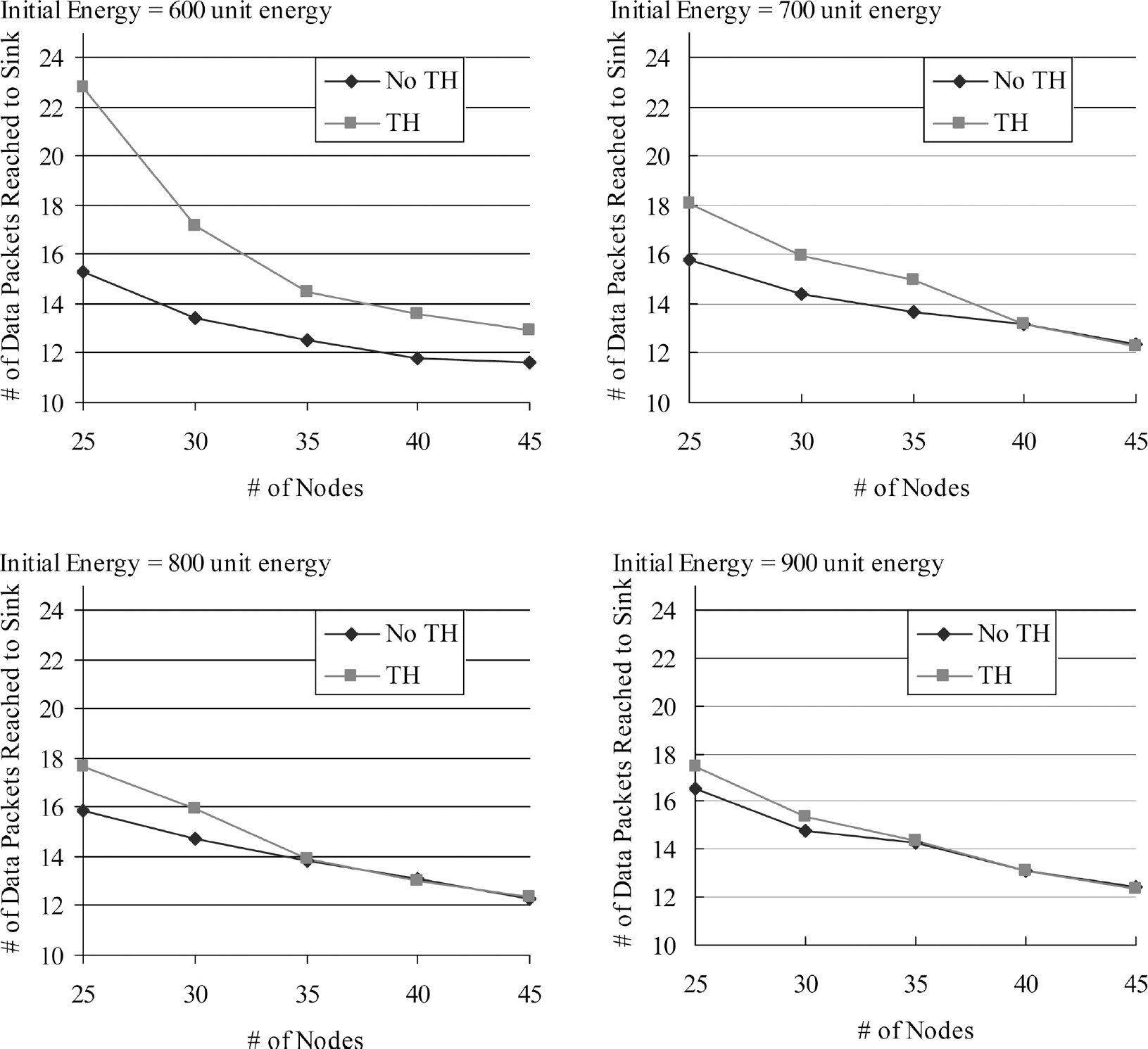
Number of data packets delivered. (a) 600 unit energy, (b) 700 unit energy, (c) 800 unit energy, (d) 900 unit energy.
Battery threshold value

If that was the case, there is no difference between a routing with and without a battery threshold value. Thus, at a larger number of nodes in a network, the number of data packets delivered by a routing with threshold value becomes close to that delivered by a routing without threshold value. In addition to that, the effect of applying a threshold value on a routing is more significant at low initial battery energy than high initial battery energy. This is due to the same reason explained above. At low initial battery energy, sensor nodes fail more quickly as compared to those at higher initial battery energy.
Figure 6 shows energy consumed by an entire network with different initial battery energy. When the initial battery energy is limited, the difference between with and without the battery threshold value is more significant, similar to that in Fig. 5. At an initial energy of 600 unit energy, a network with a threshold value obviously consumed more energy than that without a threshold value. This difference can be explained simply by the number of data packets delivered. Figure 5-(a) indicates that a network with a threshold value delivers more data packets than one without a threshold. Since delivering more data packets consumes more energy, a network with a threshold value consumed more energy than one without. Afterwards, the difference in the number of delivered data packets are reduced between with and without a threshold value as initial battery energy increases, as shown in Fig. 5. Therefore, differences in energy consumption between with and without a threshold value are reduced in Fig. 6 as initial battery energy increases.

Total Energy Consumption by a network. (a) 600 unit energy, (b) 700 unit energy, (c) 800 unit energy, (d) 900 unit energy.
Another interesting point of Fig. 6 is the change in power consumption at a given number of nodes with respect to initial battery energy. Figure 5 shows that the number of data packets delivered does not change abruptly for a given number of nodes when changing initial battery power (except at 25 nodes with initial energy of 600). However, total energy consumption by a network for a given number of nodes steadily increases as initial battery energy increases. Since the number of nodes in a network, the number of data packets delivered, and the simulation time are the same, there should be another factor, which affects energy consumption. The power consumption in the proposed scheme occurs by exchanging 1) labels, 2) request, and 3) data. If the number of data packets delivered is same, the amount of energy consumed by 2) and 3) is the same as the number of nodes and simulation times. Thus, the only possibility is due to label exchanges. When increasing initial battery energy, the number of nodes running out of batteries in a given simulation time will be reduced. Then, more nodes participate in exchanging labels. Therefore, at the higher initial battery energy, more total energy is consumed by a network.
Figure 7 shows the percentage of information packets dropped out of all sensed events. There are three different types of information packets dropping — (a) dropping label, (b) dropping request, and (c) dropping data. In the proposed scheme, a data or request packet is transmitted only once. Thus, when (b) and (c) occur in our routing scheme, a data packet never reaches a sink. However, a label packet is broadcast, so it is possible that many copies of the label packet traverse a network at the same time. Dropping one label does not mean losing all copies of the label. Therefore, when a label never reached a sink, we consider it a “dropped label.” In the case of simulation results with a threshold value, only (a) can happen. Because of a threshold value, if there is a possibility of (b) or (c) occurring, a node does not participate in information transmission at all. It is obvious that at any point a scheme with a threshold value performs better than one without a threshold value. The simulation results show that applying a threshold value on sensor nodes increases the number of data packets delivered and prevents a sensor network from dropping information packets. Since our proposed method does not require any information exchanges about their battery status between sensor nodes, there is no transmission overhead. Each sensor node has to keep track of its own battery level and compare the battery level with a threshold value every once in a while. On the other hand, because nodes have no knowledge about their neighbors' battery status, they transmit a label to neighbors indiscriminately. When a receiving node is below a threshold value, the transmission energy is totally wasted since those neighbors do not participate in the routing scheme at all.

Percentage of information packets dropped. (a) 600 unit energy, (b) 700 unit energy, (c) 800 unit energy, (d) 900 unit energy.
The demanding tininess in hardware and the energy savings carry out an extensive role in defining wireless sensor networks, a step ahead of the traditional ad hoc networks. Furthermore, specific applications necessitate redefining some of the basic paradigms with which energy aware protocols are engineered. We have presented a new energy efficient routing scheme for data dissemination in wireless sensor networks, which ensures the graceful degradation of the network in low-energy networks, thereby, enhancing the fault tolerance of the system. As part of the future work, the energy restrained routing needs to be gauged on physical hardware to establish the usefulness of the current proposal.