A Distributed Wireless Sensor Network for Radio Scene Analysis

Abstract

In this paper, a distributed approach to radio scene analysis is considered. A Wireless Sensor Network, composed by Software Defined and Cognitive terminals, is used to classify air interfaces present in the radio scene. Two modes, namely Frequency Hopping Code Division Multiple Access and Direct Sequence Code Division Multiple Access, are identified, employing a signal processing technique. Time Frequency analysis, and a distributed decision theory. Advantages given by distributed detection are used to improve the performance of a Mode Identification module. Results in terms of error probability are obtained by modelling the probability density function of considered features as Asymmetric Generalized and Generalized Gaussian functions.

Keywords

Wireless Sensor Networks Cognitive Radio Distributed Detection Radio Scene Analysis Mode Identification Wireless LAN Bluetooth

1. Introduction

In the last 5–10 years, the scientific community, under pressure from the military world (and not only the military world), is concentrating big and multidisciplinary efforts on the study of sensor networks (SN), particularly of wireless sensor networks (WSN). A SN is a group of nodes able to sense the external world and exchange the gathered information; if the medium of the communication flow is wireless, the network is called WSN. Thousands of applications can be mentioned for WSN, and four main possible fields of use can be identified: military, environmental, health, and domestic [1, 2].

The military field is the most demanding and because of this, the best performances can be found in these applications: force, equipment, and ammunition monitoring, battlefield surveillance, target identification and enemy spying, damages evaluation, nuclear, biological, and chemical (NBC) attack detection [3] are some of the possible uses.

In the environmental application, WSN are very useful because (usually) the variables to be monitored are spread in large areas which, many times, are not studied for their inaccessibility: in this case, the absence of infrastructure is overcome by the modularity of WSN allowing the user to cover the monitored area with high flexibility. Some examples can be found in [4 –8].

The third application field is the medical world, where WSN are essentially used to monitor the health status of the patient. Particular interest is devoted to embedded sensors, directly inserted in the body, which compose a network with external nodes for a continuous control of the subject. Examples can be found in [9] and [10].

The last but not least important field is the building automation. In this case, the aim is to join heterogeneous systems present in a building to create a fully-interconnected network of devices. Many applications of this kind can be found in smart spaces, domotic, and video surveillance [11, 12].

In many of the previous mentioned applications and architectures, a common part is present and fundamental for each target: the availability to exchange information by using wireless links. The advantage consists in avoiding a fixed infrastructure, but the drawback is that a radio link is usually time-varying and very noisy. The first solution is to build a network with performances, pre-defined in respect to the worst case, but this means an inefficient use of resources, such as the spectrum. Thus, nowadays the challenge is to project networks and devices able to adapt themselves to the external environment, and in particular to the radio resources (spectrum, standard, mode, etc); this paradigm is reflected by the so-called Software Defined and Cognitive Radio approach [13, 14, 15]. The Software Defined and Cognitive Radio brings to the definition a completely adaptable physical layer, where the communication features can change in relation to the conditions of the wireless channel, to the traffic status, and to the users' requirements.

2. The Problem of Radio Scene Analysis

In order to reach such fully-reconfigurable devices and networks, many issues are still open, such as powerful algorithms and procedures to understand the external “radio-scene” [15]; among them, one of the main important topics is Mode Identification and Spectrum Monitoring (MISM) [16, 17, 18]. MISM is the process through which a base station or a terminal understands the radio-scene by classifying the available transmission modes and the spectrum holes in the channel. A transmission mode (also called air interfaces [13]) can be defined as the specification of the radio transmission between a transmitter and a receiver. It defines the frequencies or the bandwidth of the radio channels, and the encoding methods used such as FH-CDMA, DS-CDMA, TDMA, MC-CDMA, etc. [13]. By using MISM, a cognitive terminal should be able to recognize the spectrum holes and the available modes in order to improve the efficiency of spectrum use and of radio resources in general. To implement the framework of a MISM module, this work proposes the use of a Wireless Sensor Network composed by Software Defined and Cognitive Radio devices.

3. Solutions for Radio Scene Analysis

In the state of the art, some proposals can be found to implement radio sensing modules. The simpler and older solution is the use of the so-called radiometer [20]. The idea is to scan spectrum by extracting energy in each sub-band identifying the presence of signals. The advantage of this approach is the very low computational load, but the drawback is that, when signals temporally overlap on the same band, energy detection can be insufficient to discriminate the mode. Moreover, the pieces of information provided by energy detection cannot be enough to take further steps. For example, in the direction of modulation recognition. Another work [16] presents the use of a radial basis function (RBF) neural network for a power spectral density estimation to identify the communication standard. No superposition of signals is considered, and different radio frequency stages are employed. In [18] a further integrated solution is proposed by means of a two step sensing module: first an energy detection to identify a void or occupied carrier; and a following Radio Access Technologies (air interface) classification to detect GSM and UMTS signals. Also in this approach, no superposition of modes is taken into account and, moreover, the solution is studied for a stand alone sensor. The first procedure for sensing and identification of overlapping modes is presented in [17], where a time frequency analysis is combined with neural network to classify spread spectrum interfaces, such as frequency hopping and direct sequence. The use of time frequency methods allows the study in the time and the frequency plane of spectrum in order to evaluate the so-called white spaces (or spectrum holes) also in time domain and, moreover, to discriminate two air interfaces using the same band. Approaches for spectrum sensing, based on time frequency analysis, have been subsequently proposed also in [15] with a complete and exhaustive analysis of cognitive radios; in that article, the author proposes a two step-procedure composed by interference temperature estimation and spectrum holes detection. Another recent work is [21], which shows an air interface classification (that is mode identification), based on cyclostationarity detection. The feature of cyclostationarity is used like a signature of superimposed modes: each signal provides this property with different frequencies and for different values of time lag and, by using binary hypothesis testing, is classified. Another related work, and probably one of the biggest efforts in the field of spectrum sensing is given by the Next Generation (XG) Program, funded by DARPA, whose goals are the improvement in assured military communications through the dynamic assignment of allocated spectrum. In the Request for Comments (RFC) section of the XG Program [22], a key function is given by sensing module, which has to sample the channel in order to determine occupancy. The criteria for declaring a channel occupied is not specified, but it is reported that the basic notion is to determine if there is a signal (frequencies usage) and if so, what the characteristics of the signal are (air interfaces classification).

This article starts with the vision of cognitive wireless sensors (Section 4), whereas in Section 5 the entire proposed framework is described. In Sections 6 and 7 procedures are explained with a deep analysis of distributed detection (Subsect. 7.2). Results and conclusions are shown in Sections 8 and 9.

4. Cognitive Wireless Sensors Network Vision

The vision proposed in this work joins two different research fields: Sensor Network and Cognitive Radios. The problem of radio scene analysis, typical of Software Defined and Cognitive Radios [15, 18, 23], is tackled starting from the solution proposed in [17] to arrive at proposing the use of Distributed Detection, typical of Sensor Network [24 –26], by considering cognitive terminal as cognitive sensor node. Through this approach, advantages of cooperative strategies and sensor networks are provided. A better performance in terms of correct detection, which cannot be reached, for stand alone sensor, with its own procedure will be shown in Section 8. Each device/sensor works together with other terminals to obtain data about wireless channel, more detailed and correct than in the stand alone scenario. To explain how this objective is reached, examples of two air interfaces. Direct Sequence Code Division Multiple Access (DS-CDMA) and Frequency Hopping Code Division Multiple Access (FH-CDMA) are classified by using distributed cooperative terminals. Two cases of study are considered: IEEE WLAN 802.11b and Bluetooth. The choice of these two standards stems from three factors: first, they are based on the chosen modes, DS-CDMA and FH-CDMA, second, they use the same bandwidth (Industrial Scientific Medical (ISM) Band) allowing the design of a unique RF conversion stage, as ideally required for an SDR platform [13]: third, the growing interest in them on the market for their wireless connectivity, especially for communications in coexistent environment.

5. General Framework and Proposed Method

The approach is a generalization of the one proposed in [17] to a multiple cooperative scenario. A number N of cognitive sensors (CS) CS_i with i = 1,2, …, N, move in an indoor environment to observe the “external world” by analyzing spectrum and searching for radio sources to be localized and identified. Each CS_i is able to extract pieces of information from the external world, analyze them, decide, and act in relation to a pre-defined cognitive cycle [14]. 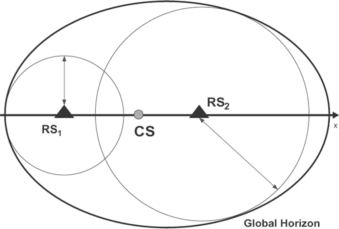More precisely, each SS captures the observation O_i (t), processes it and extracts from it a vector of features u (t) = {u₁, u₂, …, u_F}, which represents O_i in a synthetic form useful to the decision and action procedures. Each device performs a classification C_i (t) based on available observations and coopeative strategies. The classification can be defined as a mapping between a features space V and a classification space C, V is the space of possible values assumed by features extracted by each sensor during the observation C, according to pattern recognition methods, is basically a label space where labels identify different regions in the V space associated with different problem solutions. In the general framework, the classification is oriented to solve a MISM problem combined with the location estimation of sources.

The MISM and location problem is defined as follows: let us consider (Fig. 1) that a set of CSs, {CS} = {CS_i: i = 1, …, N} is present within the horizon of a number of radio sources RS_k, k = 1, …, K, where the horizon is the surface that contains all the areas of coverage of RS_k. Let us associate with each RS_k a position ${\underline{x}}_{R S_{k}}$ in a space X , and a mode m in a space of possible radio modes corresponding to different air interfaces, for example M. Let us suppose that each CS_i is associated with a position x_i in the space X, where radio sources are. Finally let's presume that no null discrete quantized observations O_ik(t), at each time t, for each sensor CS_i, are available as effects of radio source RS_k over sensor CS_i, i.e., the sensibility of each sensor CS_i is such that it can detect the presence of each radio source RS_k if only that radio source is present, supposing that all radio sources in RS space lie in the horizon of each sensor in CS. Then, the mode identification, together with spectrum monitoring and location problem, is defined as the capability of the set CS of cognitive sensors to carry out a set of classification C_i(t) about the presence of the transmission mode and the position of a set of Radio Sources RS, which lie in the horizon of S.

FIGURE 1

The general framework.

When dim{CS} = 1, a stand alone scenario is fixed, i.e., a single smart sensor is considered. If dim( X ) = 1, and the position of the stand alone CS, CS₁, are fixed, then a mono-dimensional space and horizon are considered as the world domain of the problem (Fig. 2). A situation with CS = 1 and dim(X) = 1 was considered in [17], where a feature vector v₁(t,x₁) based on time-frequency analysis of the observed spectrum, O₁(t,x₁) with CS₁ at position x₁, was analyzed. A problem with dim(RS) = 2, i.e., with two radio sources, was analyzed there with the additional constraint that ${\underline{x}}_{R S_{1}}$ and ${\underline{x}}_{R S_{2}}$ , i.e., the positions of the radio sources, were fixed. However, even though that problem allows and insight into the complexity, due to the overlapping nature of the observations O_i(t,x_i) in relation to different x _i (where the overlapping effects of sources can give rise to difficult pattern recognition problems), it is by many cases too simple to reflect more direct situations of interest. In particular, in this article some working hypothesis done in [17] are relaxed by using dim{CS} < 1 and, without loosing generality, dim {CS} = 2, where {CS} = {CS₁, CS₂} is composed by a set of two smart sensors. Let us fix dim (X) = 1 and again dim (RS) = 2, where positions of the two sources RS_k are known; in this case, the problem of localization is not present, whereas the mode identification remains the main objective of the study.

FIGURE 2

Example of stand alone seenario.

The two cognitive sensors, CS₁ and CS₂, are composed of different blocks (Fig. 3), which can be grouped in Sensing Modules and in Analysis Modules. 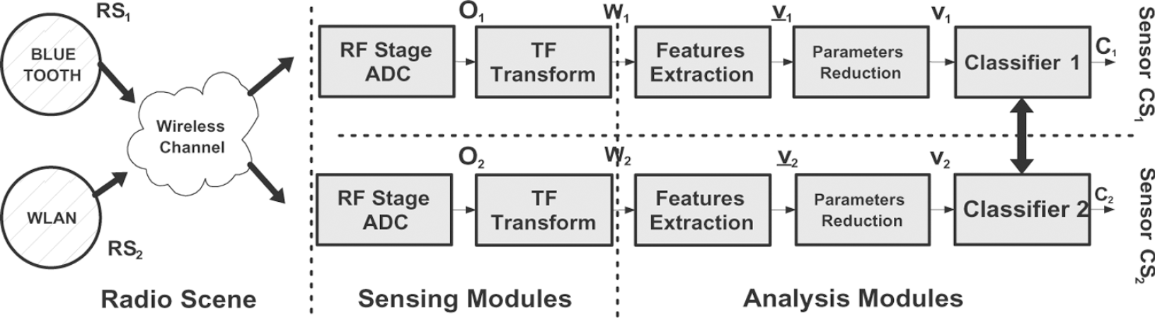The sensing procedures are performed by directly sampling the received signal and representing it in a bilinear space, the Time Frequency (TF) plane (see Section 6.1); once TF matrixes, W₁ and W₂ are obtained, the analysis procedures start: from W_i, i = 1,2, the features vector v _i is computed (see Section 7.1) and sent to the classification module (Section 7.2) which, by means of a cooperative strategy, extracts the classification C_i(t). As the classification C_i(t) is taken by these two cognitive sensors, we have to assess the nature of cooperation between the WSN. In particular, each CS CS_i could cooperate in different ways with the other CSs, CS_jj = 1,2, to take C_i(t) which, in this case, as M = 2 and dim{RS} = 2, are RS^M = 2² = 4 (see Sec. 7.2).

FIGURE 3

Logical architecture of two cooperative sensors.

6. Sensing Procedures

6.1. Time Frequency Analysis

The observation O_i(t) after Radio Frequency (RF) stage and A/D conversion is processed by a TF block. The bilinear nature of the TF transforms provides a methodology to process time-varying and superimposed signals as the ones considered in this work. As TF distribution, the Wigner-Ville transform has been chosen [27]. This transform is the most used in the state of the art, and it has low computational complexity, a good feature for real-time usage. The Wigner-Ville distribution is given by:

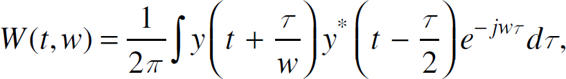
W (t, w) = \frac{1}{2 π} \int y (t + \frac{τ}{w}) y^{*} (t - \frac{τ}{2}) e^{- j w τ} d τ,

(1)

where the superscript ∗ denotes the complex conjugate, and integral ranges from −∞ to +∞ and y(t) constitute the sampled version of the received signal. It is band-limited, and contains one of the two superimposed modes (WLAN or Bluetooth), or both.

7. Analysis Procedures

7.1. Features Extraction and Reduction

From Wigner-Ville transform, it is possible to extract TF features of the received signal observed on a time window T. The same two features, used in [17] with one sensor, are considered here:

Feature 1 : standard deviation of the instantaneous frequency.

Feature 2: maximum time duration of signal.

To obtain the first feature from a given TF distribution, the first conditional moment is computed as:

< w >_{t} = \frac{1}{P (t)} \int w W (t, w) d w

(2)

where P(t) is the time distribution (time marginal), and the integral ranges go from +∞ to −∞. In our case, W(t,w) is the Wigner-Ville distribution of the received signal. < w > _t is the average of frequency at a particular time t and it is considered as the instantaneous frequency w_i [27]. The standard deviation of w_i is:

s t d (w_{i}) = \frac{1}{T} \sum (w_{i} - w_{i})^{2},

(3)

where w_i is the mean value of w_i computed on the time window T. From Fig. 4 you can see that it is reasonable to obtain a low value of std(w_i) when the first conditional moment is quite constant as in the case of DS (IEEE 802.11b), while it assumes high values in the case of FH (Bluetooth). The second feature is obtained on the basis of the following considerations: in the case of DS, frequency components are continuous in time for a duration that depends on the length of the time observation window T used to compute the distribution. Instead, for FH signal, a discontinuity in time can be observed due to the presence of different frequency hops. Therefore, it is possible to obtain an empirical discriminating feature based on the time duration of the signal. To obtain such data, the following operations are performed:

From the chosen transform, a binary TF matrix W_bin(t,w) is obtained “binarizing” W(t,w) through a threshold to eliminate noise. The values of this matrix represent presence (element equals 1) or absence (element equals 0) of a signal at a given time t and at a given frequency f.

The threshold has been chosen in an empirical way. After a trial and test procedure, its value has been chosen as the mean value of the TF matrix.

Once W_bin(t,w) has been obtained, the elements of each row, i.e., for each frequency, are summed up obtaining T(w), standing for the length in time of the component in relation to frequency.

FIGURE 4

Instantaneous frequency for the two signals, WLAN (a) and Bluetooth (b).

The feature used for the classification has been chosen as the maximum value T_M in such set, namely:

T_{M} = m a x (T (w)),

(4)

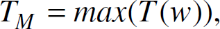
where

T (w) = \sum_{t} W_{b i n} (t, w),

(5)

in which the summation is done over the entire length of the window, where the distribution is computed.

At the end of the feature computation, a vector v is obtained:

\underline{v} = {v_{1}, v_{2}} = {s t d (w_{i}), T_{M}} .

(6)

To simplify the problem decreasing the dimension of features space, the Karhunen-Loeve (K-L) method [28] has been performed. It computes a linear transformation, identified by the matrix A[n × m], in order to reduce the dimension of features space from n dimension to m, with m > n. Once a new feature linear combination of the ones proposed in Equations (3) and (4) is obtained from K-L, simpler probability density functions (pdf) can be computed. In the case of WLAN, Bluetooth, and Noise class, the pdf can be expressed as a Asymmetric Generalized Gaussian (AGG) [29] with the form expressed in (7).

P_{a g g} (x) = {\begin{cases} \frac{c γ a}{Γ (1 / c)} e^{- γ_{l}^{c} [- (x - m_{x})]^{c}} & x < m_{x} \\ \frac{c γ a}{Γ (1 / c)} e^{- γ_{r}^{c} [x - m_{x}]^{c}} & x > m_{x}, \end{cases}

(7)

where

\begin{matrix} γ_{a} = \frac{1}{σ_{l} + σ_{r}} {(\frac{Γ (3 / c)}{Γ (1 / c)})}^{0.5} γ_{l} = \frac{1}{σ_{l}} {(\frac{Γ (3 / c)}{Γ (1 / c)})}^{0.5} \\ γ_{r} = \frac{1}{σ_{r}} {(\frac{Γ (3 / c)}{Γ (1 / c)})}^{0.5} . \end{matrix}

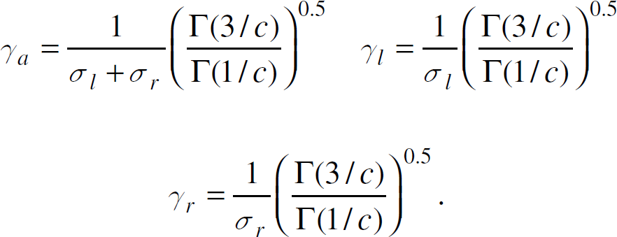
In case of WLAN and Bluetooth signal, the pdf can be modelled as a Generalized Gaussian (66) distribution [29] whose expression is obtained from (7), setting the equality between the right and left variance.

P_{g g} (x) = \frac{c γ}{2 Γ (1 / c)} e^{- | γ (x - m_{x}) |^{c}},

(8)

where

γ = \sqrt{\frac{Γ (3 / c)}{σ^{2} Γ (1 / c)}},

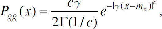
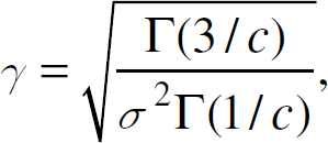
where for both distribution, (7) and (8), Γ(x) is the gamma function and the parameters are: σ² the variance, σ² _r the right variance, σ² _l the let variance, m_x the mean value. β₂ the kurtosis, and:

c = \sqrt{\frac{5}{β_{2} - 1.865}} - 0.12 i f 1.865 < β_{2} < 15.

Once pdf of feature are modelled, the detection process can be carried out. In the following Subsection the steps to reach distributed classification modules are explained.

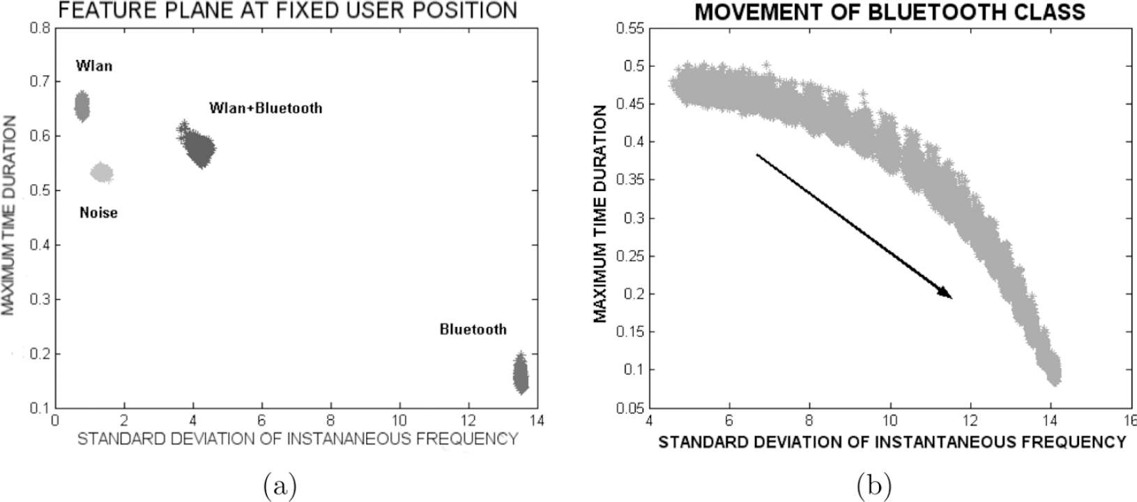
It is worth mentioning another characteristic features: as it can be noticed in Fig. 5a, when one sensor S_i is at rest in a given position x _i , the features plane assumes that representation, but when x_t changes, i.e., the considered sensor moves in the environment, then the features also change their value. An example of the feature movement, when the sensor moves away from WLAN source, is reported in Fig. 5b. This observation brings to consideration the vector v not only as a function of time t, v(t), but also of position x _i , then v(t,x_i).

FIGURE 5

Feature plane for the four class at fixed user position (a) and for the bluetooth class during the movement of one sensor (b).

7.2. Distributed Classification

As reported in Section 5, in addition to an advanced signal processing technique, i.e., the Time-Frequency analysis (Sect. 6.1), to improve the performances of the MISM module, a distributed classification algorithm is studied.

Different strategies can be designed to implement a cooperative behavior of Cognitive Sensors. In the following, two possible strategies are explained, pointing out the advantages and disadvantages of each one.

A first possible way of cooperation is to provide each sensor with multiple samples of the features vector v_i(t) at a given time t₀: these samples are used by the sensor to take its decision knowing what the other sensors are observing. This can be reached by allowing each sensor CS_i to communicate its vector r _i to another sensor CS_g, and by defining decision algorithms using multiple observations.

As v_i(t) = v_i(t,x_i) i.e, the feature vetor is a function of the position of the sensor too, the relative position of all the sensors must be known as well to allow the correct alignment of the observed patterns in the pattern space. Therefore, C_i(t) is a mapping function defined as {v_i(t,x_i)}→ C ≡ M₁ × M₂. This approach implies that information on {v_i(t,x_i), i = 1,2} is exchanged as a wireless message: the radio-frequency transmission can be overlapped to the air interfaces already present in the environment, i.e., it can be interpreted as an interfering signal on the observations O_i(t,x_i), changing the nature of observations themselves and of the problem.

Another possibility is that each element of the set of sensors shares the decision model with all the others in an a-priori way. Let us assume that each sensor knows its decision behavior, i.e., the mapping function C_i (t): this a-priori knowledge is shared in an off-line phase, i.e., no detector is immersed in the environment and no one is observing the radio scene. The exchanged information requires a significantly lower bandwidth than the previous cooperative strategy, and no signal interferes with the present radio scene. As the feature vector is a function of the position of the sensor, the classification behavior depends on the position of the node: the exchanged information can hence be coded as a probabilistic distribution of the features in the space, let us call it “features map.” This second case finds a theoretical framework in the distributed Bayesian detection by Varshney [24]. This study foresees the application of this approach with some changes to the considered scenario.

To study and implement the detection problem, it still remains to be defined which values the classification C_i (t) can assume; starting from the general framework described in Section 5, given two possible modes M₁ and M₂ and two radio sources, RS₁ and RS₂, the situations to be classified are four, and in particular:

absence of signal, when all sources (RS₁ and RS₂) are switched off and only environmental Noise (Noise class) can be present;

presence of WLAN signal (WLAN class), RS₁ is switched on, and RS₂ is switched off;

presence of Bluetooth signal (Bluetooth (BT) class), RS₁ is switched off, and RS₂ is switched on;

presence of WLAN and Bluetooth signals (WLAN and Bluetooth class), RS₁, and RS₂ are switched on.

Thus, by using the classification function C_i(t) each sensor CS_i has to extract one of the four classes from C space, composed as follows: C = {{Noise, Noise},{Noise, WLAN}, {BT, Noise}, {BT, WLAN}}, where the first component of each class is the status of RS₁ and the second one of RS₂, and Noise means the corresponding source is switched off, and only the environmental noise is present. To simplify the classification process, it is possible to reduce the problem to a binary classification test. In fact, given the position of each detector, it is possible to classify the air interface by solving a set of binary problems. The distribution of the probability density functions of the features on the K-L axis shows that only two classes are partially overlapped, and they can generate ambiguities for each subproblem.

Hence, by studying pdfs' positions in feature space after the K-L reduction. It is possible to build two binary trees. In particular, in Fig. 6 histograms and relative pdfs are plotted together showing the first configuration, which generates the first binary tree, shown in Fig. 8. Whereas, in Fig. 7, the second situation is represented, and the relative tree is in Fig. 9. It is worth mentioning (as already stated) that the movement of the class is given by the sensor's movement and, moreover, that the Bluetooth class pdf is not plotted in Figs. 6 and 7, because it is very far (in K-L axis) from the pdfs of other classes: last consideration is reported in binary trees, where the Bluetooth class is the first one, which can be classified at the first decision level.

FIGURE 6

PDFs and Histograms of classes in the first configuration.

FIGURE 7

PDFs and Histograms of classes in the second configuration.

Let us then consider a binary phenomena, i.e., two possible hypotheses are present. H₀ and H₁, in association with the a-prior probabilities, P₀ and P₁, which represent a possible couple of the previously described classes. Because y₁ and y₂ are the observations relative to the two sensors, taken at the correspondent distance x ₁ and x ₂, the local classification C_i, with i = {1,2} (where i denotes which sensor makes the classification), is given by:

C_{i} = {\begin{cases} 0 & if H_{0} declared present, \\ 1 & if H_{1} is declared present . \end{cases}

(9)

The local classification C_i is based on the local observation y_i, at a given position x _i , if no communication link is present between the two sensors (Figure 10). The cost assigned to each case of classification is given by C_ijk, i,j,k = {0,1}, and it represents the cost of sensor 1 classifying H_i, sensor 2 classifying H_j, when H_k is present. The target is to obtain a classification rule that minimizes the average cost of the classification making [24] for the considered positions of the two detectors, i.e., x ₁ and x ₂. The following Bayesian risk function is used for this purpose.

\begin{aligned} ℜ = & \sum_{i, j, k} \int_{y_{1}, y_{2}} p (C_{1}, C_{2}, y_{1}, y_{2}, H_{k} ∣ X) C_{i j k} \\ = & \sum_{i, j, k} \int_{y_{1}, y_{2}} P_{k} C_{i j k} p (C_{1}, C_{2}, y_{1}, y_{2} ∣ H_{k}, X) \\ = & \sum_{i, j, k} \int_{y_{1}, y_{2}} P_{k} C_{i j k} p (C_{1}, C_{2} ∣ y_{1}, y_{2}, H_{k}, X) \\ . p (y_{1}, y_{2} ∣ H_{k}, X), \end{aligned}

(10)

where the dependance from the distance X = {x_i, i = 1,2} is added to [24].

FIGURE 8

The first binary decision tree used by each sensor.

FIGURE 9

The second binary decision tree used by each sensor.

FIGURE 10

Parallel decision performed by two sensors of a binary phenomenon.

Because the local classifications C₁ and C₂ are independent and based respectively on the local observation y₁ and y₂, and on the positions of the sensors x ₁ and x ₂, it is possible to express the risk function as follows:

ℜ = \sum_{i, j, k} \int_{y_{1}, y_{2}} P_{k} C_{i j k} p (C_{1} ∣ y_{1}, {\underline{x}}_{1}) p (C_{2} ∣ y_{2}, {\underline{x}}_{2}) p (y_{1}, y_{2} ∣ H_{k}, X) .

(11)

Explicitly summing over C₁, by considering that:

p (C_{1} = 1 ∣ y_{1}, {\underline{x}}_{1}) = 1 - p (C_{1} = 0 ∣ y_{1}, {\underline{x}}_{1})

(12)

and by ignoring the constant terms with respect to C₁, it's possible to re-write ℜ:

ℜ = \int_{y_{1}} p (C_{1} = 0 ∣ y_{1}, {\underline{x}}_{1}) \sum_{j, k} \int_{y_{2}} P_{k} p (C_{2} ∣ y_{2}, {\underline{x}}_{2}) p (y_{1}, y_{2} ∣ H_{k}, X) [C_{0 j k} - C_{1 j k}] .

(13)

It's now possible to derive a classification rule for sensor 1 [24]:

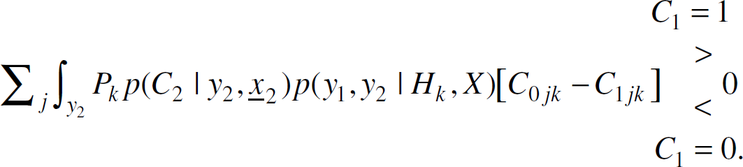
\sum_{j} \int_{y_{2}} P_{k} p (C_{2} ∣ y_{2}, {\underline{x}}_{2}) p (y_{1}, y_{2} ∣ H_{k}, X) [C_{0 j k} - C_{1 j k}]_{\underset{C_{1} = 0 .}{<}}^{\overset{C_{1} = 1}{>}} 0

(14)

Expanding the sum over k, the following formula can be obtained [24]:

\begin{aligned} \sum_{j} \int_{y_{2}} P_{0} p (C_{2} ∣ y_{2}, {\underline{x}}_{2}) p (y_{1}, y_{2} ∣ H_{0}, X) [C_{0 j 0} - C_{1 j 0}]_{\underset{C_{1} = 0}{<}}^{\overset{C_{1} = 1}{>}} \\ \sum_{j} \int_{y_{2}} P_{1} p (C_{2} ∣ y_{2}, {\underline{x}}_{2}) p (y_{1}, y_{2} ∣ H_{1}, X) [C_{0 j 1} - C_{1 j 1}] . \end{aligned}

(15)

Assuming the cost of sensor 1, making an error when H₀ is present, is more than the cost of classifying correctly regardless of the classification of sensor 2, i.e., C_0j0 < C_1j0, and by considering that:

p (y_{1}, y_{2} ∣ H_{k}, X) = p (y_{2} ∣ y_{1}, H_{k}, X), k = 0, 1

(16)

(15) can be expressed as a likelihood ratio test [24]:

Λ (y_{1}) {_{<}^{>}}_{_{C_{1} = 0,}}^{^{C_{1} = 1}} \frac{P_{0} \sum_{j} \int_{y_{2}} p (C_{2} ∣ y_{2}, {\underline{x}}_{2}) p (y_{2} ∣ y_{1}, H_{0}, X) [C_{1 j 0} - C_{0 j 0}]}{P_{1} \sum_{j} \int_{y_{2}} p (C_{2} ∣ y_{2}, {\underline{x}}_{2}) p (y_{2} ∣ y_{1}, H_{1}, X) [C_{0 j 1} - C_{1 j 1}]}

(17)

where Λ (y₁ is the Bayesian likelihood function for detector 1:

Λ (y_{1}) = \frac{p (y_{1} ∣ H_{1}, {\underline{x}}_{1})}{p (y_{1} ∣ H_{0}, {\underline{x}}_{1})} .

(18)

The previous equation (17) shows that the right-hand side is a function not only of the observation for sensor 1, i.e., y₁, but it is possible to note that it is a function of C₂, i.e., the classification rule for sensor 2 also and this dependence appears under the form of p(C₂|y₂, x₂).

Under the hypothesis of the conditional independence of y₁ and y₂, i.e., when

p (y_{2} ∣ y_{1}, H_{k}, {\underline{x}}_{1}, {\underline{x}}_{2}) = p (y_{2} ∣ H_{k}, {\underline{x}}_{2}),

(19)

the right-hand side of (17) can be reduced to a threshold given by [24]:

t_{1} = \frac{P_{0} \sum_{j} \int_{y_{2}} p (C_{2} ∣ y_{2}, {\underline{x}}_{2}) p (y_{2} ∣ H_{0}, {\underline{x}}_{2}) [C_{1 j 0} - C_{0 j 0}]}{P_{1} \sum_{j} \int_{y_{2}} p (C_{2} ∣ y_{2}, {\underline{x}}_{2}) p (y_{2} ∣ H_{1}, {\underline{x}}_{2}) [C_{1 j 1} - C_{1 j 1}]} .

(20)

Noting that

p (C_{2} = 1 ∣ y_{2}, {\underline{x}}_{2}) = 1 - p (C_{2} = 0 ∣ y_{2}, {\underline{x}}_{2}),

(21)

it's possible to expand (20) in order to show explicitly that t₁ is a function of p(C₂ = 0|y₂, x₂), which represents the classification rule for sensor 2. A similar conclusion can be obtained for the threshold of sensor 2.

The proposed general definition and optimization of the whole system involves the existence of two coupled thresholds even if there is no communication link between the two detectors; but for the setup considered in the present paper, an offline exchange of information consisting in p(C_i = 0|H_j, x_i) where i = 1,2 and; j = 0,1 is performed (See Fig. 11).

FIGURE 11

Structure of a distributed detection system.

Let us now consider a special assignment of the costs as follows [24], where the cost value doesn't depend on which sensor makes the error:

\begin{aligned} C_{000} = C_{111} = 0 \\ C_{010} = & C_{100} = C_{011} = C_{101} = 1 \\ C_{001} = C_{110} = k . \end{aligned}

(22)

The resulting threshold for sensor 1 becomes [24]:

t_{1} = \frac{(k - 1) + (2 - k) p (C_{2} = 0 ∣ H_{0}, {\underline{x}}_{2})}{1 + (k - 2) p (C_{2} = 0 ∣ H_{1} {\underline{x}}_{2})} .

(23)

A similar expression can be used to compute the threshold for sensor 2. These obtained thresholds are, in general, different from the ones computed if each sensor was considered independently.

Given the position of the sensor, it's possible to apply the binary tree shown in Figs. 8 and 9, transforming the M-ary classification problem into a binary one.

For each likelihood function, it is possible to consider two different cases, i.e., both p(y_i | H_j, x_i) and p(y_i | H_k, x_i) are modelled as generalized gaussians, or, in alternative, one is a generalized gaussian, and the other one is an asymmetric generalized gaussian. In the first case, the decision rule can be written as:

\sum_{n = 1}^{N} [- | γ_{j} (y_{n} - m_{j}) |^{c_{j}} + | γ_{k} (y_{n} - m_{k}) |^{c_{k}}]_{\underset{u_{i} = 0}{<}}^{\overset{u_{i} = 1}{>}} \ln (\frac{c_{k} γ_{k}}{2 Γ (1 / c_{k})}) - \ln (\frac{c_{j} γ_{j}}{2 Γ (1 / c_{j})}) + \ln t_{i} .

(24)

A similar expression can be obtained even in the second case, but the right side and the left side of the asymmetric gaussian have to be treated separately, because a different variance is involved for each side [29].

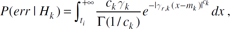
In the off-line phase, after computing the thresholds t₁ and t₂, it's possible to define an error probability conditioned to each class (denoting with i = {1,2} the sensor, and with k = {0,1,2,3} the class)

if t_i > m_k:

P (e r r ∣ H_{k}) = \int_{t_{i}}^{+ \infty} \frac{c_{k} γ_{k}}{Γ (1 / c_{k})} e^{- | γ_{r, k} (x - m_{k}) |^{c_{k}}} d x,

(25)

if t_k < m_k:

P (e r r ∣ H_{k}) = \int_{- \infty}^{t_{i}} \frac{c_{k} γ_{k}}{Γ (1 / c_{k})} e^{- | γ_{l, k} (x - m_{k}) |^{c_{k}}} d x .

(26)

In the following paragraph the simulation environment, based on previously described assumptions, the theoretical error probability for the moving sensor CS_i, and a comparison with a stand alone case are shown.

8. Results

The general scenario explained in Section 5 is implemented by using Matlab/Simulink. In particular, two cognitive sensors, CS₁ and CS₂, are used, as shown in Fig. 12, moving around a room of 15 m × 15 m. The radio scene to be detected can be composed by either one of two possible modes, M₁ or M₂ (Direct Sequence Code Division Multiple Access (DS-CDMA) or Frequency Hopping Code Division Multiple Access (FH-CDMA)), or both, or none of them. The two modes are implemented, taking into account all parameters defined in the standards [30,31], except for protocols higher than the physical layer. The radio channel is modelled as indoor multipath with AWGN. Multipath model is Rice fading with delay spread of 60ns, and root mean square (rms) delay spread of 30ns [32]. A path loss term has been inserted: it follows the model proposed in [33]. This is composed of two parts: for distances lower than 8m, the path loss L_p has a value dependent on frequency f and on the distance d from the source; for distances larger than 8m, L_p is only a function of d. The attenuation is obtained by:

L_{p} = {\begin{cases} 32.45 + 20 \log (f . d) & d \leq 8, \\ 58.3 + 33 \log (d / 8) & d > 8, \end{cases}

(27)

where d is expressed in meters, and f in GHz.

FIGURE 12

Considered indoor scenario.

The received signals, corrupted by AWGN and multipath and attenuated as reported above, are then translated in IF at 30 MHz with a sample rate of 120 Msample/s to satisfy the Nyquist limit. Then they are computed by TF block: the Wigner-Ville distribution uses blocks with N = 512 samples, obtained through a time window T large enough to contain 10 frequency hops. The time hopping is 625 μs. The extraction module stores 10 TF matrices, and it calculates the features as expressed in Section 7.1. Then the features are reduced with K-L method (Section 7.1), and their pdfs are modelled as AGG and GG. Due to the relation between the feature vector ν and the sensor position x _i , a study of statistical parameters of pdfs in different sensor positions has been carried out. For instance, the behavior of variance and mean value of feature of Bluetooth class is shown in Fig. 13. This study has been developed for each of the four classes obtaining all parameters in function of sensor position, and inserting them in pdf general formula. At the end of this step, the distributions, i.e., Generalized or Asymmetric Generalized Gaussian, are available for all the considered scenario. With these data the detection can be carried out computing the Error Probability as explained below. This approach arises a problem: the sensor CS_i has to be aware of its position. In this work, this quantity is assumed to be known, but ongoing research is dealing with a methodology to relax this constraint applying methods for hidden parameters estimation.

FIGURE 13

Parameters of feature (after KL reduction) for bluetooth class in relation to user's distance from WLAN source. Variation (a), mean value (b).

To have a clear idea of the improvement of performances given by the proposed distributed system, in the following figures error probabilities, both for cooperative and stand alone scenarios, are shown.

In Fig. 14, error probabilities are compared for the couple WLAN+Bluetooth and Noise, computed in case of one sensor at rest at 8.5m from the WLAN source, and the other one moving from 2m up to 12m on the line of sight between the two access points: the cost k of the double error is taken equal to 10. Two error probabilities are shown in the figure: one represents the probability of classifying WLAN+Bluetooth instead of Noise when all sources are switched off, and the other one represents the probability of deciding the presence of only Noise while WLAN + Bluetooth is present. In both cases, the error probability increases, reaching a peak at about 8 m from the WLAN source; this fact is due to an overlap of the two cases that generates ambiguities in the decision process. In Fig. 15, it is possible to see the error probability for the classes WLAN + Bluetooth and Noise for the stand alone scenario. It is possible to see a worst performance than in the cooperative scenario, where, for instance, the value of 10⁻¹⁰ is maintained within a distance of 7m, while, in this case, it is held within 6.5m. Moreover, the overall behavior is characterized by a higher Error Probability than the one obtained with distributed detectors.

FIGURE 14

Error probability of WLAN+Bluetooth and Noise classes for the cooperative scenario.

FIGURE 15

Error probability of WLAN+Bluetooth and Noise classes for the stand alone scenario.

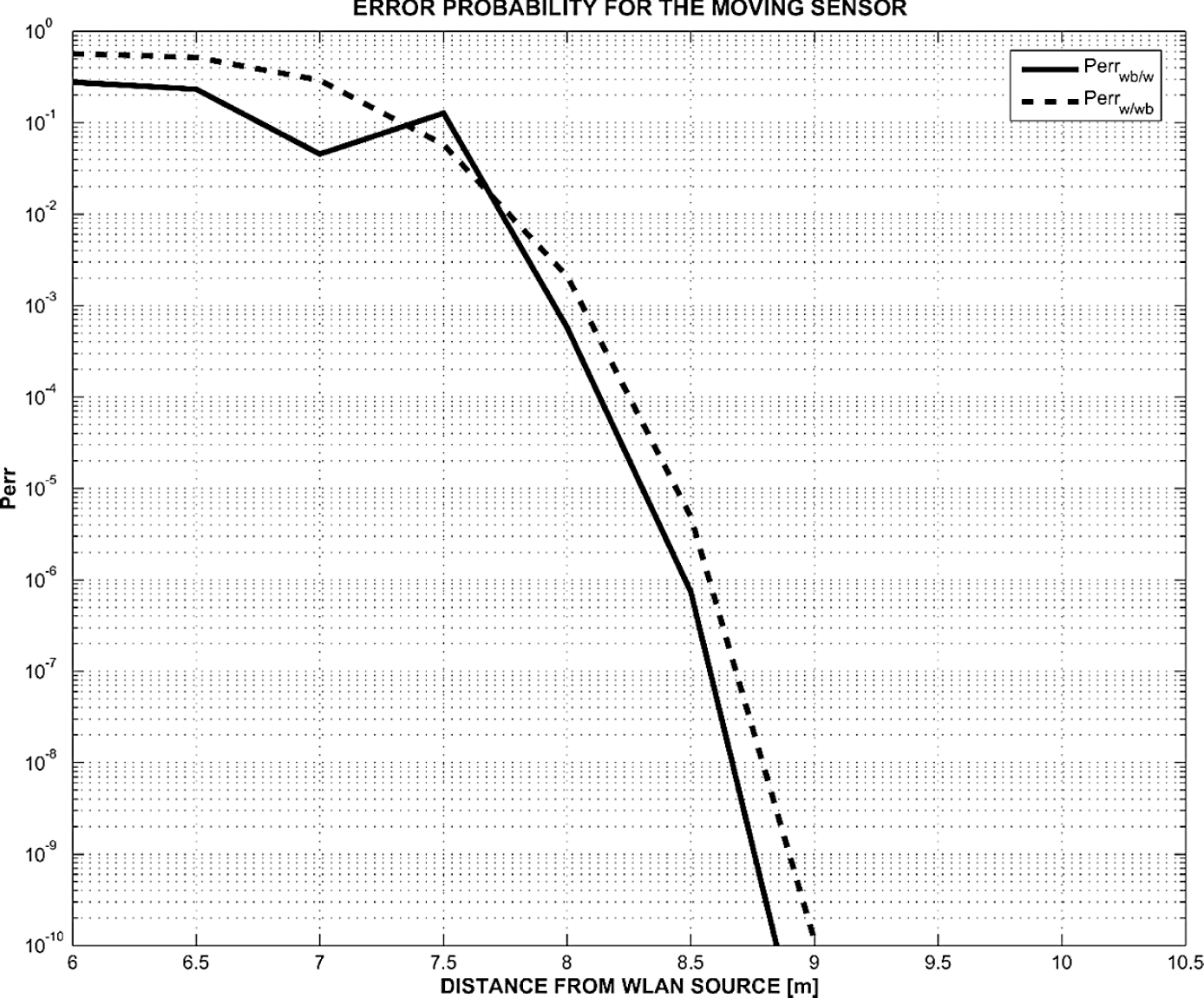
In Fig. 16, the error probabilities computed for the couple WLAN – Bluetooth and WLAN for the following scenario are presented: one detector fixed at 3.5m from the WLAN 802.11b source, and the other one moved from 2m up to 12m on the line of sight between the two access points; the cost of double error, even in this case, is taken equal to 10. For both cases (identifying WLAN when WLAN + Bluetooth is present and viceversa), the maximum ambiguity has been obtained for distances close to the WLAN source, where the classes are strongly overlapped. Also in this case the system presents good performances, and the closed form of the error probability, (25) and (26), allows an objective evaluation, biased by the fitting error and by K-L reduction, of the proposed algorithm. The improvement of cooperative case with respect to stand alone scenario is clear as it can be noticed in Figs. 16 and 17.

FIGURE 16

Error probability of WLAN and WLAN+Bluetooth and Noise classes for the cooperative scenario.

FIGURE 17

Error probability of WLAN and WLAN + Bluetooth classes for the stand alone scenario.

9. Conclusion

The paper deals with a distributed decision approach to solve the problem of Mode Identification in the context of Cognitive Wireless Sensor Networks. Two air interfaces have been considered to be classified, namely Frequency Hopping Code Division Multiple Access and Direct Sequence Code Division Multiple Access. A binary and distributed likelihood test has been computed obtaining a closed form for error probability in case of Generalized and Asymmetric Generalized Gaussian probability density function. Shown results demonstrate good performance of proposed approach. Ongoing research is centered on the resolution of multiple hypothesis distributed decision test, taking into account new air interfaces such as multi-carrier techniques, and new methodologies for a joint estimation of position and modes.

References

Akyildiz

I. F.

Sankarasubramaniam

, and Cayirci

, “Wireless Sensor Networks: A Survey,” Computer Networks Journal, 38, 4, 393–422, March, 2003.

Kumar

Zhao

, and Shepherd

, “Special Issue on Collaborative Signal and Information Processing in Microsensor Networks,” IEEE Signal Processing Mag., Mar 2002.

Kumar

, and Shepherd

, “Sensit: Sensor Information Technology for the Warfighter,” Proc. Forth Int. Conf. On Information Fusion, 2001.

Polastre

Szewczyk

, and Mainwaring

, “Analysis of Wireless Sensor Networks for Habitat Monitoring”, in Wireless Sensor Networks pp. 399–423, Kluwer Academic Publishers, 1st edition, 2004.

Martinez

, “Sensors Network Applications,” IEEE Computer, 37, 8, 50–56, August, 2004.

Holman

, “Applying Video Sensor Networks to Nearshore Environment Monitoring,” IEEE Pervasive Computing, 2, 4, 14–21, April, 2003.

Grismer

M. E.

, “Field Sensor Networks and Automated Monitoring of Soil-Water Sensors,” Soil Science, 154, 6, 482–489, July, 1992.

Alley

R. B.

, “Continuity Come First: Recent Progress in Understanding Subglacial Deformation,” in Deformation of Glacial Materials, 171–180, Geological Soc. of London, 2000.

Yang

B.-H.

Rhee

, “Development of the Ring Sensor for Healthcare Automation.” Robotics and Autonomous Systems, 30, 3, 273281, 2000.

10.

Amato

, “Health Care Monitoring of Mobile Patients,” ERCIM News, 60, 69–70, January, 2005.

11.

Foresti

G. L.

Regazzoni

C. S.

, and Varshney

, Multisensor Surveillance Systems. The Fusion Perspective. Kluwer Academic Publishers, 2003.

12.

Regazzoni

C. S.

, “Intelligent Fusion of Visual, Radio and Heterogeneous Embedded Sensors' Information within Cooperative and Distributed Smart Spaces,” in Data Fusion for Situation Monitoring, Incident Detection, Alert and Response Management, NATO Science Series, Kluwer Academic Publishers, 2005.

13.

Mitola

, Software Radio Architecture: Object-Oriented Approaches to Wireless Systems Engineering. John Wiley and Sons, New York, NY, 2000.

14.

Mitola

, “Cognitive Radio: Making Software Radio More Personal,” IEEE Pers. Comm., 6, 4, 48–52, August, 1999.

15.

Iiaykin

, “Cognitive Radio: Brain-Empoweres Wireless Communications,” IEEE Journal Sel. Areas in Comm., 23, 2, 201–220, February, 2005.

16.

Palicot

, and Roland

, “A New Concept for Wireless Reconfigurable Receivers,” IEEE Communications Magazine, 41, 7, 124–132, July, 2003.

17.

Gandetto

Guainazzo

, and Regazzoni

C. S.

, “Use of Time-frequency Analysis and Neural Networks For mode Identification in a Wireless Software-defined Radio Approach,” Eurasip Journal of Applied Signal Processing, Special Issue on Non Linear Signal Processing and Image Processing, 13, 1778–1790, Oct., 2004.

18.

Vardoulias

, and Faroughi-Esfahani

., “Mode Identification and Monitoring of Available Air Interfaces,” in Software Defined Radio; Architectures, System and Functions. 329–352, John Wiley and Sons Ltd., April, 2003.

19.

Kolodzy

, “Next Generation Communications: Kickoff Meeting,” in Proc. DARPA. 2001.

20.

Urkowitz

, “Energy Detection of Unknown Deterministic Signals,” Proceedings of IEEE, 55, 4, 523–531, April, 1967.

21.

Oner

, and Jondral

, “Air Interface Recognition for a Software Radio System Exploiting Cyclostationarity,” 15th IEEE International Symposium on Personal, Indoor and Mobile Radio Communications, 2004. PIMRC 2004, 3, 1947–1951, Sept., 2004.

22.

BBN Technologies.

“XG Architectural Framework RFC,” Cambridge, Massachusetts, USA, 2003.

23.

Mitola

, Cognitive Radio: An Integrated Agent Architecture for Software Defined Radio, Ph.D. Thesis, Royal Institute of Technology (KTH), Sweden, May, 2000.

24.

Varshney

P. K.

, “Distributed Detection and Data Fusion,” in 3-Distributed Detection Without Fusion. Springer-Verlag, 1st edition, 1996.

25.

Xiao

J. J.

, and Luo

Z.-Q.

, “Universal Deceontralized Detection in a Bandwidth-constrained Sensor Network,” IEEE Transaction on Signal Processing, 53, 8, 2617–2624, August, 2005.

26.

Camberland

J. F.

, and Veeravalli

V.V.

, “Decentralized detection in sensor network,”.

27.

Cohen

, Time Frequency Analysis: Theory and Applications, Prentice-Hall Signal Processing. Prentice Hall PTR, 1st edition, December, 1994.

28.

Fukunaga

, Introduction to Statistical Pattern Recognition. Academic Press Inc., 2nd edition edition. 1990.

29.

Tesei

, and Regazzoni

C. S.

, “Hos-based Generalized Noise pdf Models for Signal Detection Optimization,” Signal Processing, 65, 2, 267–281, March, 1998.

30.

IEEE , IEEE 802.11b, Wireless LAN MAC and PIIY specifications: higher speed physical layer (PIIY) extension in the 2.4GHz band, supplement to 802.11 edition, 1999.

31.

Bluetooth SIG, Inc. , Bluetooth standard, Specification of the Bluetooth System, v 1.2 edition, November, 2003.

32.

Wysocki

T. A.

Zepernick

H. J.

, “Characterization of the Indoor Radio Propagation Channel at 2.4 ghz,” Journal of Telecommunications and Information Technology, 1, 3–4, 8490, 2000.

33.

Kamerman

, “Coexistence between Bluetooth and IEEE 802.11 CCK Solutions to Avoid Mutual Interference,” Tech. Rep., Lucent Technologies, Bell Laboratories, January, 1999.