Sage Journals: Discover world-class research

Abstract

This paper assumes a set of identical wireless hosts, each one aware of its location. The network is described by a unit distance graph whose vertices are points on the plane two of which are connected if their distance is at most one. The goal of this paper is to design local distributed solutions that require a constant number of communication rounds, independently of the network size or diameter. This is achieved through a combination of distributed computing and computational complexity tools. Starting with a unit distance graph, the paper shows: 1. How to extract a triangulated planar spanner; 2. Several algorithms are proposed to construct spanning trees of the triangulation. Also, it is described how to construct three spanning trees of the Delaunay triangulation having pairwise empty intersection, with high probability. These algorithms are interesting in their own right, since trees are a popular structure used by many network algorithms; 3. A load balanced distributed storage strategy on top of the trees is presented, that spreads replicas of data stored in the hosts in a way that the difference between the number of replicas stored by any two hosts is small. Each of the algorithms presented is local, and hence so is the final distributed storage solution, obtained by composing all of them. This implies that the solution adapts very quickly, in constant time, to network topology changes. We present a thorough experimental evaluation of each of the algorithms supporting our claims.

Keywords

Backup Protocol Delaunay Triangulation Distributed Dynamic Storage Spanning Tree Unit Disk Graph Wireless Network

1. Introduction

The problem of storing multiple copies of files in different parts of a network has been widely studied since the early 70s, see [7] for a thorough survey. It provides a classic solution to reduce response time for data, increase availability, and improve general fault-tolerance. The remarkable growth of reliable and efficient networking over the past few decades has fostered the development of distributed storage systems. A recent issue of IEEE Internet Computing [25] devoted to this area describes various approaches taken by distributed storage systems, including storage virtualization, peer-to-peer, and server-to-server.

A. Data Storage in Wireless Networks

This paper develops distributed storage solutions for mobile wireless networks. It assumes a set of n identical wireless hosts in the plane, each one aware of its location, either from a GPS system or through other means, such as inertial sensors and acoustic range-finding devices. Two hosts can communicate if they are within a fixed distance, say one unit. Thus in our paper, a wireless network can be described as a geometric graph whose vertices are points on the plane (our wireless hosts) two of which are connected if their distance is at most one, i.e. it is a unit distance graph.

Since the topology of wireless networks is constantly changing, and the nodes have location awareness, protocols for wireless networks differ significantly from standard solutions used in wired networks. In addition, wireless devices have much lower bandwidth and limited power supplies. Therefore, protocols for wireless networks should use as little communication as possible and should run as fast as possible; even traditional solutions that have only a linear cost in the diameter of the network may not be acceptable. The goal of this paper is to design local distributed solutions that require a constant number of communication rounds, independently of the network size or diameter.

The absence of a central infrastructure, together with the highly dynamic nature of wireless networks, imply that such networks do not have an associated fixed topology. An important task is to determine an appropriate topology over which high-level protocols are implemented; see [22] for a survey of various topology control methods. Algorithms that allow to establish and maintain an energy efficient connected constant degree overlay network have been described in e.g. [9], [13], [14], [24]. Starting with a unit distance graph, this paper extracts a triangulated planar spanner through the local algorithm of [14], and then proposes several algorithms inspired by the method of [2] to construct a spanning tree of the triangulation. Both algorithms are local and hence adapt in constant time to network topology changes.

B. Related Results and Applications of Data Storage

An interesting application of the storage protocols described in this paper is the problem of reliably storing global snapshots of the state of a distributed system (e.g. [6], [8]). Snapshots of a distributed system can be used, for example, for system recovery after a problem (e.g. deadlock) is detected. A strategy for reliably storing data such as snapshots can consider spatial redundancy, temporal redundancy, or a combination of both. In spatial redundancy each snapshot is replicated and spread among a number of processors, in a way that if at most t processors fail, the snapshot can be recovered; e.g. storing several copies in different processors, or spreading each copy into several pieces using coding based strategies; see [10], [21] and references herein. In temporal redundancy a few, say k, of the latest snapshots, are stored in different processors; for recovery the latest available snapshot is used. Either way, since snapshots may be rather large (each one contains the local state of every processor in the system), it is convenient to design balanced strategies that distribute the load evenly among the processors. This work improves upon the solutions to the snapshot storage problem of [16], where static strategies are computed off-line using combinatorial design theory.

Papers such as [10], [11] have proposed coloring based solutions for mobile networks for a different storage problem, that requires that every node has replicas nearby; these solutions are not local.

C. Outline and Results of the Paper

The goal of this paper is to design local distributed storage solutions that require a small number of communication rounds, independently of the network size or diameter. This is achieved through a combination of distributed computing and computational complexity tools, that make heavy use of the fact that nodes know their locations, and the geometry of the plane. The solutions proposed here are built up from two layers: a spanning tree maintenance protocol, and a load-balanced storage backup protocol. Various spanning tree protocols are proposed, which are interesting in their own right: trees are a popular form of network structure that are used by many network algorithms. The backup protocols allow each node to replicate data to neighboring nodes for fault-tolerance, such that the difference in the number of copies each node stores is small. A thorough experimental study is presented, that analyzes the properties of the trees, and of the performance of the backup protocols on top of the trees.

The protocols described in this paper also show how to construct locally three spanning trees whose union is the Delaunay triangulation of the given pointset, with high probability. A virtual ring can be maintained by traversing the tree in DFS order. This ring easily adapts to network changes, deletions and additions of processors can be handled locally and on the average in constant time.

The backup protocol that stores data in consecutive nodes on the virtual ring, according to various policies, is presented. Notice that once the tree is obtained, leader election can be performed using only a linear number of messages.¹ This is the first algorithm that matches the Ω(n log n) lower bound of [23] for leader election in a geometric ring of size n.

Finally, we have simulated all our algorithms and in Section 4 we provide detailed results of our simulations for a wireless network produced from 200 nodes generated at random. Our simulations indicate the effectiveness and adaptability of the algorithms proposed in this paper.

2. Algorithm for Distributed Dynamic Storage

Assume a set of n wireless hosts in the plane, each of which is aware of its location. The main feature of our algorithm is that dynamic storage is attained and subsequently maintained by cooperating nodes that use only “local” knowledge, i.e., information about themselves and their distance one neighborhood nodes. In outline, our proposed distributed dynamic storage algorithm itself is in two phases. In the first phase the input unit disc graph is processed in order to produce first a triangulated planar spanner (using a Localized Delaunay Triangulation algorithm [14]) and from there a tree spanner is obtained using the Entry-Edge Elimination criteria introduced in [2]. In the second phase a cycle is embedded into the tree spanner and subsequently our dynamic storage procedure is applied.

A. Preprocessing Procedures

In this section we review the techniques necessary to preprocess the wireless network. We need two key components. The first one, a technique to extract a spanning tree of a planar geometric graph, and a method to extract from a unit distance graph, the local Delaunay subgraph, which under the right conditions is the same as the Delaunay triangulation of the points of a unit distance graph.

1) Delaunay and Localized Delaunay Triangulation

Let the hosts have identical radius r_n and let G(P, r_n) denote the unit disc graph on a set P of n nodes. The parameters we chose are guided by the main result of Penrose [17], [18] which guarantees k-connectivity.

The result implies that for any real number c if $r_{n} \geq \sqrt{\frac{\ln n + c}{n π}}$ then the probability the network G(P, r_n) is connected is at leat $\geq e^{- e^{- c}}, as n \to \infty$ . If we substitute e^c = s and recall that $e^{- e^{- c}} \approx 1 - e^{- c}$ then we see that

Pr [Network G (P, r_{n}) is connected] \geq 1 - \frac{1}{s},

(1)

for $r_{n} \geq \sqrt{\frac{\ln n + \ln s}{n π}}$

The Delaunay triangulation cannot be computed “locally”. In the sequel, we will require that our construction is based only on local operations by the hosts. It has been proved by Bern et al. [3] (see also Li et al. [15]) that if the reachability radius of the hosts is chosen so as to satisfy Inequality 1 then with high probability the Delaunay triangulation is the same as the localized Delaunay triangulation. We review their argument in the sequel. The probability that a region R of area |R| has exactly l nodes from the random poinset obeys the Poisson ditribution and is equal to

\frac{(n | R |)^{l}}{l!} e^{- n | R |} .

Let d_n be the random variable that denotes the length of the longest edge of the Delaunay triangulation of the random pointset. If d_n ≥ d then there is a triangle in the triangulation at least one of whose edges is ≥ d and whose circumcircle contains no other points of the random poinset: note that the area of this circumcircle is at least $π d^{2} / 4$ . Since the Delaunay triangulation of a set of n points has at most 3n triangles we conclude that $Pr [d_{n} \geq d] \leq 3 n e^{- n π d^{2} / 4}$ . If we put $1 / t = 3 n e^{- n π d^{2} / 4}$ , solve for d and substitute in the last inequality then we see that

Pr [d n < \sqrt{\frac{4 (\ln n + \ln t + \ln 3)}{n π}}] \geq 1 - \frac{1}{t} .

(2)

If we now put s = n⁸ in Inequality 1, and t = n in Inequality 2 then we see that $Pr [d_{n} < r_{n}] \geq 1 - \frac{1}{n}$ , for $r_{n} \geq \sqrt{\frac{9 \ln n}{n π}}$ , i.e., the longest edge of the Delaunay triangulation is smaller than r_n with probability at least $1 - \frac{1}{n}$ .

The Unit Delaunay triangulation (denoted by UDel(P, r_n)) is the graph obtained by removing all edges of the Delaunay triangulation which are longer than r_n. Note that using only their local information nodes of a given triangle alone can decide together whether or not they form a triangle. A triangle is k-localized if all its edges have a length at most of 1 and also the interior of its circumcircle contains no point of P that is a k-neighbor of its vertices. The k-localized Delaunay graph (denoted by LDel^(k)(P, r_n)) consists of exactly the Gabriel edges and edges of the k-localized Delaunay triangles [15]. It has been shown [14] that LDel^(k) (P, r_n) is planar for k ≥ 2, while LDel⁽¹⁾ (P, r_n) may not be planar. However, there is an algorithm that can remove intersections from LDel⁽¹⁾ (P, r_n) in order to produce the planarized Delaunay Triangulation (denoted by PLDel(P, r_n)). The planarization of LDel⁽¹⁾ (P, r_n) essentially involves the following operations.

Each node u gathers the location information of its distance one neighborhood (including u itself) and computes its Delaunay Triangulation.

The node u computes all triangles with all edges at most one unit and broadcasts a message to form a Delaunay triangle if the angle of the triangle formed at u is at least /3.

Node u accepts a proposal if the triangle proposed is in its Delaunay triangulation and has been proposed by both neighbors of the proposed triangle. For more details see Alzoubi et al. [1]. In view of our previous discussion we have the following result.

Proposition 2.1

If $r_{n} \geq \sqrt{\frac{9 \ln n}{n π}}$ then the planarized Delaunay triangulation with radius r_n is the same as the Delaunay triangulation of P with probability at least $1 - \frac{1}{n}$ .

2) Tree extraction in planar subdivisions

Let P be a simple polygon embedded on the plane, and let l be the vertical line tangent to P such that P lies to the left of l. Then the entry edge of P is the lowest edge of P that touches l. See Fig. 1.

Let G be a plane geometric graph, that is a planar graph embedded on the plane such that its edges are represented by line segments joining pairs of points representing the vertices of G. G partitions the plane into a set of faces one of which is unbounded. Each face f of G, but the external one defines a polygon. The entry edge of f is the entry edge of its corresponding polygon. Let T_G be the graph obtained from G by removing the entry edge of all its faces, albeit the external one. The following result is proved in [2].

Proposition 2.2

T_G is a plane spanning tree of G.

FIGURE 1

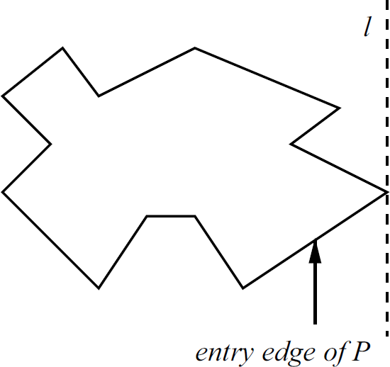
An example illustrating the definition of the entry edge of a polygon.

This extraction technique is useful for general planar subdivisions. In the sequel we will develop new and more efficient “localized” algorithms for extracting trees.

3) Tree extraction in convex subdivisions

Graphs all of whose faces, but the outer one are convex, are called convex subdivisions. If in addition all the faces of G with the exception of the outer one are triangles, G is called a triangulation. The following observation is straightforward: If G is a convex subdivision then T_G can be obtained as follows: For every vertex v of G consider the set of edges to the left of v whose rightmost vertex is v. Remove from G all of them, but the topmost. We can refer to this as the leftmost-topmost elimination rule. Similarly, a topmost-rightmost elimination rule can be obtained follows: for every vertex v of G consider the set of edges whose bottom vertex is v. Remove from G all of them, but the rightmost. In a similar way we can define a rightmost-bottommost and bottommost-leftmost elimination rules, each of which defines a sparning tree of G.

Our previous observation allows us to carry out the extraction of a spanning tree in a planar subdivision in a fully distributed way, in fact if v is a vertex of a convex subdivision all it has to do is to eliminate all the edges incident to it, except the top edge to its left. Let G be a triangulation whose vertex set is a point set P with n elements. Assume that P has k of its elements on its convex hull. Let T_G and T'_G be the spanning trees obtained by applying the leftmost-topmost and the topmost-rightmost elimination rules respectively to G. The following result is easy to prove.

Proposition 2.3

T_G and T'_G, have at most $k + \frac{n - k}{2}$ edges in common.

As a direct consequence we also have.

Proposition 2.4

Let G be a wireless network (modeled as a unit distance graph). Then using local operations at each node of G, we can maintain a plane spanning tree of G.

Proof

Using the algorithms presented in Alzoubi et al. [1] we first calculate the localized Delaunay triangulation of G. Then using the leftmost-topmost elimination rule obtain a plane spanning tree T_G of G. Since both steps can be achieved using only local operations at each node of G, the extraction of T_G can be done in a local way.

Since for points placed on the plane at random with the uniform distribution the expected number of points on the convex hull of P is [20]:

Θ(ln n) for points chosen in a convex polygon, and

$Θ (\ln n)$ for points chosen in a convex region with doubly differentiable boundary, we can conclude that in general T_G and T'_G will have, in the worst case, aproximately n/2 edges in common.

Distance-based tree extraction. As we will see, it turns out that distance based tree extraction is more efficient. Motivated from our experimental analyis in Section 4 we will explore the following new rules for tree extraction whereby all nodes (except the righmost one) are connected to a neighbor to their right. In the sequel consider the convex subdivision formed by the Delaunay triangualtion. In the Max distance left to right (MaxDLTR) tree each node is connected to a max distance neighbor to its right; in the Min distance left to right (MinDLTR) tree each node is connected to a min distance neighbor to its right; finally, in the Mid distance left to right (MidDLTR) tree each node is connected to a neighbor other than a Max or Min neighbor to its right (if it has one) else to the Max. It turns out that with high probability these three trees contain all the edges of the Delaunay triangulation with high probability, asymptotically in n. To be more precise we can prove the following result.

Proposition 2.5

Assume $r_{n} \geq \sqrt{\frac{9 \ln n}{n π}}$ and consider the trees MinDLTR, MaxDLTR, and MidDLTR. Then the probability that any pair among these trees has an edge in common is at most 1/n, asymptotically in n.

Proof

As in Proposition 2.1 the probability that a region R of area |R| has exactly l nodes from the random poinset obeys the Poisson ditribution and is equal to $\frac{(n | R |)^{l}}{l!} e^{- n | R |}$ . Consider a given edge e, say e: = {u, v} that is common to both trees MaxDLTR and MinDLTR. It follows that node u, say, has only one neighbor to its right, namely v. Since the reachability radius of the nodes is r_n, it follows from the definition of the tree MaxDLTR that v is the max distance neighbor of u and therefore the region determined by the semicircle centered at u and radius r_n (call this region S) contains exactly one point from the given pointset P. Hence, $Pr [e occurs in both trees] = n | S | e^{- n | S |} = \frac{n π_{n}^{2}}{2} e^{- n π r_{n}^{2} / 2} \leq \frac{n π}{n^{9 / 2}} = \frac{π}{n^{7 / 2}}$ . Since the Delaunay triangulation has at most 3n edges it follows that the probability the two trees have an edge in common is at most $1 / n^{2}$ , asymptotically in n.

A similar proof will work for any other pair of trees. For example, for the trees MaxDLTR and MidDLTR if a given edge e: = {u, v} is common to both then the semicircle centered at u and radius r_n will have at most two points from the pointset. Threfore an upper bound on the probability that an edge is common can be obtained easily as in the previous analysis using the Poisson distribution. We leave the details to the reader. This completes the proof of Proposition 2.5.

We note two useful consequences of Proposition 2.5 for the three trees MaxDLTR, MaxDLTR, and MidDLTR and under the assumption that $r_{n} \geq \sqrt{\frac{9 \ln n}{n π}}$ . First, the union of the trees is the Delaunay triangulation of the pointset P with probability at least 1 − 1/n, asymptotically in n. Second, for any two among these trees, the expected number of common edges is constant. This follows easily from the well-known identity $E [X] = \sum_{k} Pr [X > k]$ , where X is the random variable that counts the number of edges common to the two trees. We also note that as a consequence of a result by Bose et al. [4], the diameter of a Delaunay triangulation on a random set of n points is $O (\sqrt{n})$ .

Other rules for tree extraction. In distance-based tree extraction a node must search all its neighbors and select the one that is furthest, nearest, etc. A simpler tree extraction algorithm is to have each node select a neighbor to its right (respectively, left) at random, if it has one. Another one is to have each node select its neighbor forming a slope that is minimal with the horizontal. This gives rise to the trees RLTR, RRTL, and HorDLTR, respectively, that have also been considered in our experimental results described in Section 4.

B. Distributed Dynamic Storage Algorithm

We proceed now to show how to solve the dynamic storage problem for wireless networks. We remark again that our algorithms are local, in the sense that any node in the network only knows that it is a member of a unit distance wireless network, and at any time it communicates only with its neighbors.

We observe first that the dynamic storage problem has an easy solution if G is an oriented cycle, that is if the vertices of G are labeled (v₀, …, v_m–1) such that v_i is adjacent to v_i+1, i = 0,…, m − 1 (here addition is modm). Since our goal is to store a predetermined number k of copies of a data set S_i stored at v_i, this can be accomplished by sending S_i to a predetermined set of vertices $v_{i + j 1}, \dots, v_{i + j_{k}}$ . However, extracting a hamiltonean cycle in a wireless network in a fully distributed way, i.e. in such a way that a vertex can only communicate with its neighbors seems to be an impossible task. We use instead the following method: Let T be a geometric plane tree. If we walk around T as we would in a preorder traversal of T, we define in a natural way a cycle with m = 2n − 1 vertices in which every edge of T appears twice (thus traversing an Eulerian tour), and each vertex appears as many times as its degree in T.

1) Storage backup protocols

Now we can give two storage backup protocols. In the sequel T_G denotes any of the trees constructed in Section 2-A. We choose an integer parameter k representing the number of copies to be stored in various nodes of the network. The size of k can vary but also depends on the desired fault tolerance for data recovery required. Let F_k(u) be the set of nodes to which node u forwards its data for storage. In general, the set F_k(u) is generated locally by node u and the generation procedure is part of the forwarding algorithm that is common to all participating nodes. The forwarding set is of size k.

Storage Backup Protocol> (SBP(k))

Embed a ring topology into T_G by performing a “geometric” DFS-based preorder traversal that uses the geometric identities of the nodes.

Each node u forwards its data to the nodes of the set F_k(u).

Observe that this embedding can be executed “locally” and the forwarding strategy does not prevent non-leaf nodes from receiving multiple copies of a data file originating from the same node.

It is easy to adapt the forwarding procedure so as to avoid repetitions by decrementing a counter every time a copy is received by a “new” node. For example, we can consider the following algorithm.

Non-Repetitive Storage Backup Protocol (NRSBP(k))

Embed a ring topology into T_G by performing a “geometric” DFS-based preorder traversal that uses the geometric identities of the nodes.

Each node u forwards its data to the nodes of the set F_k(u). A given node accepts the data forwarded to it only if it has not yet received other data from the same node. Else it forwards its data to its forward node in the ring.

There are two ways to affect the desired reliability of recovery. One is the size of the parameter k: the more copies are stored to other nodes the higher the reliability. Second is the choice of nodes to which node u forwards its data: this is determined by the set F_k(u) and makes load balancing possible. For example, one can choose to store the data to k consecutive forward positions either “close” to u or “further away” from u or move them to k forward random positions in order to achieve higher load balance.

In the sequel we consider three possibilities for the forwarding set F_k(u) at u: each node u selects the set F_k(u) of k nodes according to one of the following rules (note that all nodes select the same rule).

Forwarding Rules

Consecutive Forwarding (CF) Rule:

F_k(u) = {u +1 mod n, u + 2 mod n,…,u + k mod n}, i.e., node u forwards its data to its k “successive” neighbours in the oriented cycle.

Distant Consecutive Forwarding (DCF) Rule:

F_k(u) = {u + d +1 mod n, u + d + 2 mod n,…,u + d + k mod n}, i.e., for some fixed value d (signifying distance d away from u) node u forwards its data to k “successive” nodes at distance d away from itself in the oriented cycle.

Random Forwarding (RF) Rule:

F_k(u) = {u +t₁ mod n, u +t₂ mod n,…,u + t_k mod n}, where t₁, t₂,…,t_k are random values in the range 1 m generated by node u, i.e., node u forwards its data to k random locations in the oriented cycle, where the integer m is chosen so that k² = o(m).

3. Properties of the Storage Backup Protocol

In this section we discuss properties satisfied by our protocol, namely load balancing and failure recovery.

A. Load Balance

The load balancing attained by the algorithm depends not only on the forwarding algorithm but also on the topology of the wireless network.

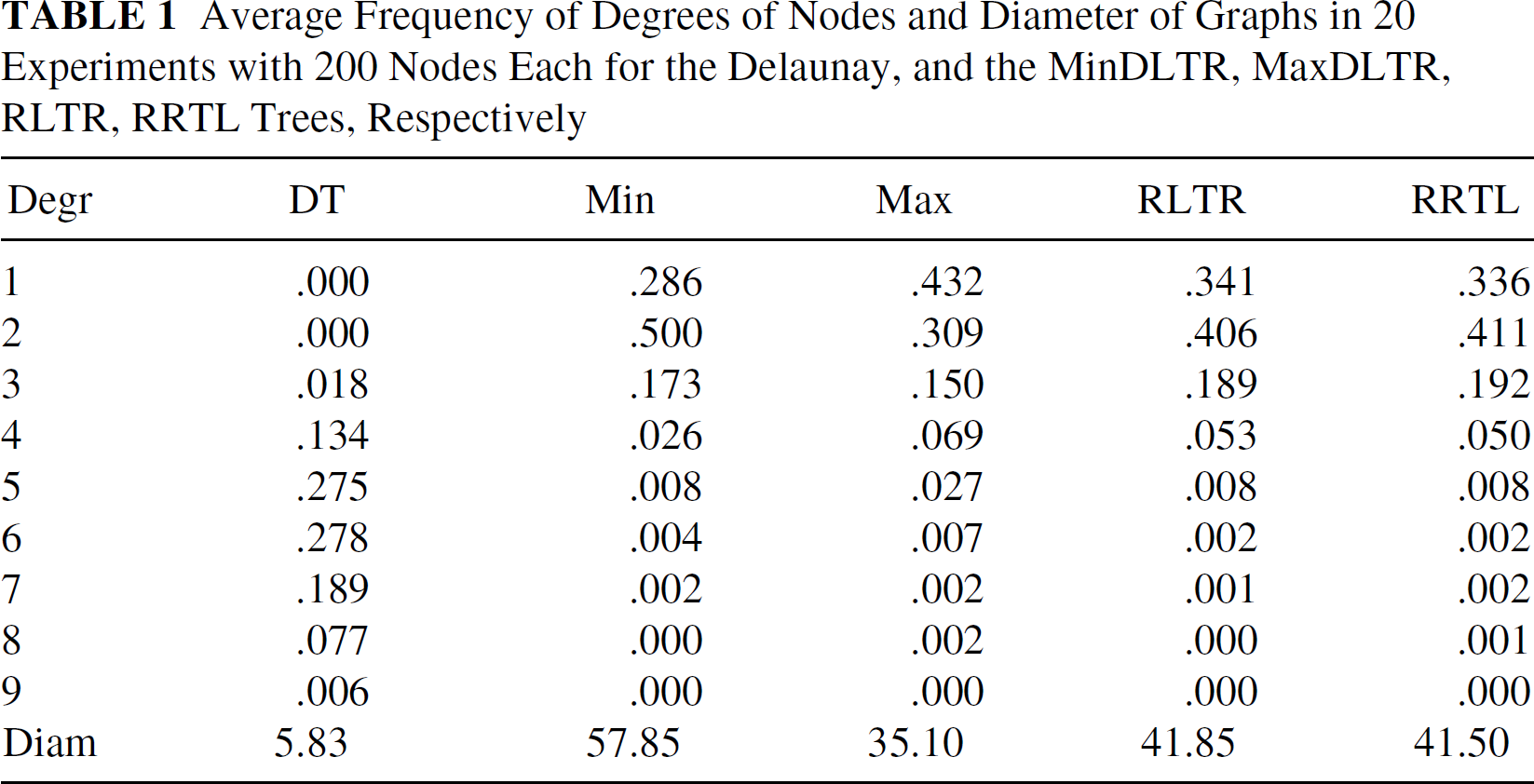
In general, experimental results indicate (see Table 1) that the spanning tree T_G obtained from G has small degree. Therefore on the average case the preorder traversal on T_G will generate a ring topology such that each node of the network is repeated a small number of times.

Let us analyze the performance of the forwarding protocols. First consider the non-repetitive storage backup protocol. If c is the max degree of the spanning tree every node of the resulting ring will store at most kc copies of other nodes' data. In particular we have the following result.

TABLE 1
Average Frequency of Degrees of Nodes and Diameter of Graphs in 20 Experiments with 200 Nodes Each for the Delaunay, and the MinDLTR, MaxDLTR, RLTR, RRTL Trees, Respectively

Degr DT Min Max RLTR RRTL

1 .000 .286 .432 .341 .336

2 .000 .500 .309 .406 .411

3 .018 .173 .150 .189 .192

4 .134 .026 .069 .053 .050

5 .275 .008 .027 .008 .008

6 .278 .004 .007 .002 .002

7 .189 .002 .002 .001 .002

8 .077 .000 .002 .000 .001

9 .006 .000 .000 .000 .000

Diam 5.83 57.85 35.10 41.85 41.50

Degr	DT	Min	Max	RLTR	RRTL
1	.000	.286	.432	.341	.336
2	.000	.500	.309	.406	.411
3	.018	.173	.150	.189	.192
4	.134	.026	.069	.053	.050
5	.275	.008	.027	.008	.008
6	.278	.004	.007	.002	.002
7	.189	.002	.002	.001	.002
8	.077	.000	.002	.000	.001
9	.006	.000	.000	.000	.000
Diam	5.83	57.85	35.10	41.85	41.50

Proposition 3.1

For each node u let S(u) be the number of data stored at u. The non-repetitive Storage backup protocol achieves load balancing in the sense that for all nodes u, v, |S(u) — S(v)|≤ ck.

A similar result also holds for repetitive loads. A trivial upper bound for the maximum absolute difference between loads can be obtained by overestimating the load. Assume a node v with degree c. We can compute load(v) by adding the storage-requests of c different directions. Notice that only k nodes for each direction can request from node v to store one unit of data. On the other hand, the nodes of only one direction can upload to node v up to c units of data each, the nodes of only one direction can upload up to c − 1 units of data each, etc. By adding the uploads and since the minimum load of a node might be zero, we have the following simple proposition.

Proposition 3.2

For each node u let S(u) be the number of data stored at u. The repetitive Storage backup protocol guaranties that for all nodes u, v,

| S (u) - S (v) | \leq \frac{k c (c - 1)}{2} .

B. Repetitive Versus Non-Repetitive Loads

One may think that non-repetitive Storage backup protocols should guarantee lower maximum difference between loads, but this is not always true. To see why, consider the family of trees on n + 6 nodes depicted in Figure 2, and assume k = 2. The eulerian tour arising is v₁v₂…v_n 1 2 3 4 3 2 5 6 5 2 1 v_n…v₂v₁

The minimum load over the nodes obtained by both protocols is zero. The repetitive Storage backup protocol loads node 2 with 4 units of data, while the non-repetitive backup protocol loads the same node with 6 units of data. Finally it is easy to see that these loads are the maximum that are obtained by each protocol.

However, in most cases, non-repetitive Storage backup protocols outperform repetitive storage backup protocols. This is also confirmed by our experimental analysis in Section 4.

C. Recovery from Failure

The resulting network failure recovery depends on the backup protocol used. In the sequel we look at properties of NRSBP(k).

FIGURE 2

A family of trees on n + 6 nodes, where n ≥ 1.

1) Single node failure

For every node of the network there is a backup of its data in at least k other nodes of the network. Therefore our protocol is k − 1 fault tolerant. In particular we have the following lemma.

Proposition 3.3

The Non-repetitive storage backup protocol NRSBP(k) is k − 1 fault tolerant, i.e., if at most k − 1 nodes fail then the data of every other node of the network is stored in at least one non-failed node.

2) Random failures

The protocol is robust under random failures. Assume that all the nodes of a random set S of size m (where m ≥ k) fail. A given node stores copies of its data into k other nodes of the network. The probability that at least one of these nodes is not in S is 1 minus the probability that they are all in S. The probability that a given node is in S is m/n, and the probability that all k nodes are in S is (m/n)^k. In particular, we have the following result.

Proposition 3.4

Assume that all the nodes of a random set S of m (where m > k) nodes fail. The probability that all the data of a given node are stored at some non-failed node of the network is at least $1 - \frac{m^{k}}{n^{k}}$ .

3) Failures of geographical regions

Our protocol can easily be adapted so that it is robust to geographic failures, that is failures created by events such as power failures that may affect the set of nodes belonging to a connected region of the plane. Consider the case of a “civilized” unit disc graph, i.e., any pair of nodes is at a distance at least X from each other, where λ > 0 is independent of n, the size of the network. Assume that all the nodes in a geographic region R of area A fail. Since the unit disc graph is civilized, the region can have at most A/λ nodes. Therefore if k ≥ A/λ then every node u within the region R has a backup of its data in at least one node outside the region R. In particular we have the following result.

Proposition 3.5

Assume that the unit disc graph is civilized with parameter λ. If all the nodes of a geographic region of area at most kλ fail then the data of each node within the region have been stored in at least one node outside the region.

4. Simulations and Experiments

In this section we provide simulations of the algorithms proposed in the previous sections and confirm experimentally the efficiency of our proposed techniques for a location aware wireless network.

A. Random Setting

First we discuss our choice of parameters in the experimental results.

1) Connectivity, Delaunay and planarized triangulations

Let the hosts have identical radius r_n and let G(P, r_n) denote the unit disc graph on a set P of n nodes. Starting from a random set P of n points, we compute their Delaunay Triangulation. As indicated in Subsection II-A.1 if we select $r_{n} \geq \sqrt{\frac{9 \ln n}{n π}}$ then the longest edge of the Delaunay triangulation is smaller than r_n with probability at least $1 - \frac{1}{n}$ , i.e., with high probability the planarized Delaunay and Delaunay triangulations are the same (see Proposition 2.1).

FIGURE 3

Delaunay triangulation and trees resulting from a random set of 200 points.

2) Spanning trees and forwarding rules

From the Delaunay triangulation we compute spanning trees using the edge extraction algorithms in Subsection 2-A.3. We then implement the storage backup protocol with three different forwarding rules as in Subsection 2-B. In the random forwarding rule the nodes will forward their data to k other processors. If k values are chosen randomly and independently with the uniform distribution in the range 1.m then it is well-known from the “birthday paradox” that the probability that no collision will occur is at least $1 - \frac{k (k - 1)}{2 m}$ . Note that the size n of the network is in general not known to the individual nodes. Given k, the value m must be chosen so that there is low probability of collision among the k random numbers t₁, t₂,…, t_k: to achieve this it is enough to guarantee that k² = o(m).

B. Results of the Simulations

Figure 3 depicts output of our experiments. From top-to-bottom and left-to-right, the first row depicts a set of 200 points chosen at random and the next picture their Delaunay. The trees depicted are formed from the Delaunay triangulation using the edge elimination rules described in Subsection 2-A.3.

The statistics reported in Table 1 give the average frequency of degrees of nodes and diameter of graphs in 20 experiments with 200 nodes chosen at random each for the Delaunay and the MinDLTR, MaxDLTR, RLTR, RRTL trees, respectively.

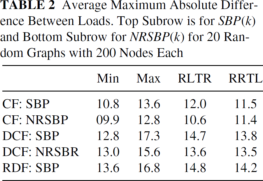
Table 2 and Table 3 illustrate the load averages for the three storage backup algorithms proposed for both the storage backup protocol SBP(k) and the non-repetitive storage backup protocol NRSBP(k). Table 2 gives the average maximum absolute difference between loads and Table 3 the average difference between loads over all pairs of nodes. These tables depict the consecutive (CF: k = 4), distant-consecutive (DCF: k = 4, d = n/2), and random distant (RDF: k = 4) forwarding rules for cycles generated from the MinDLTR, MaxDLTR, RLTR, RRTL trees, respectively, in 20 experiments with 200 nodes each. Note that the CF forwarding rule outperforms DCF and RDF, however it forwards data “near” the node initiating the forwarding. The tables also indicate that the MinDLTR tree has best performance (the second best performing tree was HorDLTR but we do not exhibit these results here).

Figure 4 depicts a histogram of the average performance of the SBP and NRSBP algorithms performed 20 times each in graphs of 100 to 200 random points in increments of 50, respectively. The top picture shows the average difference among pairs of nodes while the bottom picture the max absolute difference among pairs of nodes. Each pair of columns indicates the performance of SBP (light-gray column) and NRSBP (heavy-gray column) for the CF, DCF, and RCF forwarding rules, respectively: note that in RCF we implemented only SBP. Observe that the max absolute difference increases a little while the average absolute difference among pairs of nodes remains almost unchanged.

TABLE 2
Average Maximum Absolute Difference Between Loads. Top Subrow is for SBP(k) and Bottom Subrow for NRSBP(k) for 20 Random Graphs with 200 Nodes Each

Min Max RLTR RRTL

CF:SBP 10.8 13.6 12.0 11.5

CF:NRSBP 09.9 12.8 10.6 11.4

DCF:SBP 12.8 17.3 14.7 13.8

DCF:NRSBR 13.0 15.6 13.6 13.5

RDF:SBP 13.6 16.8 14.8 14.2

	Min	Max	RLTR	RRTL
CF:SBP	10.8	13.6	12.0	11.5
CF:NRSBP	09.9	12.8	10.6	11.4
DCF:SBP	12.8	17.3	14.7	13.8
DCF:NRSBR	13.0	15.6	13.6	13.5
RDF:SBP	13.6	16.8	14.8	14.2

TABLE 3

Average Difference Between Loads over all Pairs of Nodes. Top Subrow is for SBP(k) and Bottom Subrow for NRSBP(k) for 20 Random Graphs with 200 Nodes Each

	Min	Max	RLTR	RRTL
CF: SBP	2.43	2.92	2.67	2.62
CF: NRSBP	2.15	2.52	2.30	2.31
DCF: SBP	3.15	3.14	3.05	2.97
DCF: NRSBP	3.08	2.92	2.91	2.84
RDF: SBP	3.02	3.31	3.09	3.01

FIGURE 4

Performance of SBP (light-gray column) and NRSBP (heavy-gray column) for the CF, DCF and RCF forwarding rules.

5. Conclusion

In this paper we proposed efficient solutions to the distributed storage problem in wireless networks and designed local distributed storage solutions that require a constant number of communication rounds, independently of the network size or diameter. This is achieved through a combination of distributed computing and computational complexity tools, that make use of location awareness, i.e., that nodes know their locations, and the geometry of the plane.

Footnotes

1

The algorithm works also in a planar graph that is not a triangulation, with complexity O(f log f) in the size f of the largest face of the network.

References

Alzoubi

X.-Y.

Wang

Wan

P. -J.

, and Frieder

, “Geometric spanners for wireless Ad hoc networks,” JEEE Transactions on Parallel and Distributed Systems, 14, 5 May, 2003.

de Berg

van Kreveld

van Oostrum

, and Overmars

, “Simple traversal of a subdivision without extra storage,” Int. J. of Geographic Information Systems, 11, 359–373, 1997.

Bern

Eppstein

, and Yao

, “The expected extremes in a delaunay triangulation,” in Proc. of the 18th International Colloquium on Automata, Languages and Programming, Lecture Notes in Computer Science, 510, 674–685, 1991.

Bose

, and Devroye

, “Intersections with random geometric objects,” Computational Geometry: Theory and Applications, 10, 3, 139–154, 1998.

Bose

Morin

Stojmenovic

, and Urrutia

, “Routing with guaranteed delivery in ad hoc wireless networks,” in Proc. of Discrete Algorithms and Methods for Mobility (DIALM'99), 48–55, 1999.

Chandy

K. M.

, and Lamport

, “Distributed snapshots: Determining global states of distributed systems,” ACM Transactions on Computer Systems, 3, 1, 63–75, 1985.

Dowdy

L. W.

, and Foster

D. V.

, “Comparative models of the file assignment problem,” ACM Computing Surveys, 14, 2, 287–313, June, 1982.

Garg

V. K.

, Elements of Distributed Computing. Wiley: IEEE Computer Society Press, 2002.

Jia

Rajaraman

, and Scheideler

, “On local algorithms for topology control and routing in ad hoc networks,” in Proceedings of the 15th Annual ACM Symposium on Parallel Algorithms and Architectures, 220–229, June, 2003.

10.

Jiang

, and Bruck

, “Diversity coloring for distributed storage in mobile networks,” Technical Report, California Institute of Technology, 2001.

11.

B.-J.

, and Rubenstein

, “Greedy approach to replicated content placement using graph coloring,” in SPIE ITCom Conference on Scalability and Traffic Control in IP Networks II, Boston, MA, 289–298, July, 2002.

12.

Kranakis

Singh

, and Urrutia

, “Compass routing on geometric networks,” in Proceedings of 11th Canadian Conference on Computational Geometry, Vancouver, 51–54, August, 1999.

13.

X.-Y.

Wan

P.-J.

Wang

, and Frieder

, “Sparse power efficient topology for wireless networks,” J. Parallel and Distributed Computing, to appear.

14.

X. -Y.

Calinescu

Wan

P.-J.

, and Wang

, “Localized delaunay triangulation with application in ad hoc wireless networks,” IEEE Trans. on Par. Dist. Systems, (Modified version of the INFOCOM'2002 paper). 2003. To appear.

15.

X.-Y.

Wang

Frieder

, “Localized routing for wireless ad hoc networks,” in Proceedings of IEEE ICC, 2003.

16.

Marceln-Jimnoz

Rajsbaum

, “Cyclic strategies for balanced and fault-tolerant distributed storage,” in Proceedings LADC 2003: Lecture Notes in Computer Science #2847, Springer, 214–233, 2003.

17.

Penrose

M. D.

, “On k-connectivity for a geometric random graph,” Random Structures and Algorithms, 15, 145–164, 1999.

18.

Penrose

M. D.

, “The longest edge of the random minimal spanning tree,” The Annals of Applied Probability, 7, 2, 340–361, 1997.

19.

Perkins

C. E.

ed., Ad Hoc Networking. Addison Wesley, 2001.

20.

Preparata

, and Shamos

, “Computational geometry, an introduction.” Springer-Verlag, 1985.

21.

Rabin

M. O.

, “Efficient dispersal of information for security, load balancing and fault tolerance,” Journal of the ACM, 36, 2, 335–348, 1989.

22.

Rajaraman

, “Topology control and routing in ad hoc networks: A Survey,” SIGACT News, 33, 60–73, June, 2002.

23.

Rajsbaum

and Urrutia

, “Some problems in distributed computational geometry,” 6th International Colloquium on Structural Information and Communication Complexity (SIROCCO), Lacanau, France, July 1999; Proc. in Informatics 5, Gavoille

Bermond

J-C.

Raspaud

(Eds.), Carleton Scientific Press, 233–248. To appear in Theoretical Computer Science.

24.

Song

W. -Z.

Wang

, and Li

X. -Y.

, “Localized algorithms for energy efficient topology in wireless ad hoc networks,” in 5th ACM Int. Symp. on Mobile ad hoc Networking and Comp. Tokyo, Japan, 98–108, 2004.

25.

Yianilos

P. N.

, and Sobti

, “The Evolving Field of Distributed Storage,” IEEE Internet Computing, September–October, 35–39, 2001.

Distributed Dynamic Storage in Wireless Networks

Abstract

Keywords

1. Introduction

A. Data Storage in Wireless Networks

B. Related Results and Applications of Data Storage

C. Outline and Results of the Paper

2. Algorithm for Distributed Dynamic Storage

A. Preprocessing Procedures

1) Delaunay and Localized Delaunay Triangulation

Proposition 2.1

Proposition 2.2

Proposition 2.3

Proposition 2.4

Proof

Proposition 2.5

Proof

B. Distributed Dynamic Storage Algorithm

1) Storage backup protocols

Storage Backup Protocol> (SBP(k))

Non-Repetitive Storage Backup Protocol (NRSBP(k))

3. Properties of the Storage Backup Protocol

A. Load Balance

Proposition 3.1

Proposition 3.2

C. Recovery from Failure

Proposition 3.3

2) Random failures

Proposition 3.4

3) Failures of geographical regions

Proposition 3.5

4. Simulations and Experiments

A. Random Setting

1) Connectivity, Delaunay and planarized triangulations

B. Results of the Simulations

Footnotes

1

References