Sage Journals: Discover world-class research

Abstract

Seasonal decomposition analyses were applied to the statistical evaluation of an oscillating activity for a plasma membrane NADH oxidase activity with a temperature compensated period of 24 min. The decomposition fits were used to validate the cyclic oscillatory pattern. Three measured values, average percentage error (MAPE), a measure of the periodic oscillation, mean average deviation (MAD), a measure of the absolute average deviations from the fitted values, and mean standard deviation (MSD), the measure of standard deviation from the fitted values plus R-squared and the Henriksson-Merton p value were used to evaluate accuracy.

Decomposition was carried out by fitting a trend line to the data, then detrending the data if necessary, by subtracting the trend component. The data, with or without detrending, were then smoothed by subtracting a centered moving average of length equal to the period length determined by Fourier analysis. Finally, the time series were decomposed into cyclic and error components. The findings not only validate the periodic nature of the major oscillations but suggest, as well, that the minor intervening fluctuations also recur within each period with a reproducible pattern of recurrence.

Keywords

biological clock decomposition analyses ultradian rhythm temperature compensation circadian rhythm cultured cells

INTRODUCTION

A growth factor- and hormone- or drug-responsive oxidation of NADH catalyzed by a family of NOX proteins has been associated with plant and animal plasma membranes (ECTO-NOX proteins) (Brightman et al. 1988, 1992). In rat hepatomas (Bruno et al. 1992) and in cancer cells in culture (Morré et al. 1995a), a constitutively activated component of NADH oxidation is observed that is no longer dependent on hormone activation. This constitutively activated component is responsive to certain drugs such as the antitumor sulfonylurea, LY181984 (Morré et al. 1995b), and the capsaicinoid quinone site inhibitor capsaicin (Morré et al. 1995a, 1996). Both the constitutive and the constitutively activated oxidation of NADH exhibit properties of a NADH protein disulfide reductase (Chueh et al. 1997) and are differentially responsive to thiol reagents (Morré and Morré 1995; Morré et al. 1995c). Subsequently, the cell surface plasma membrane NADH oxidase was shown to have properties of a protein disulfide-thiol interchange protein (Morré et al. 1997). These proteins are now referred to as ECTO-NOX proteins because of their cell surface location and to distinguish them from the phox-NOX proteins of host defense (Lambeth et al. 2000).

An unusual property of both the oxidation of NADH and of the protein disulfide-thiol interchange activity catalyzed by the ECTO-NOX proteins is that both activities oscillate with a period length of 24 min (Morré and Morré 1998). Similar oscillations were observed with the NADH oxidase activity of the ECTO-NOX protein from CHO (Pogue et al. 2001) and HeLa (Wang et al. 2001) cells. With all three examples, the period length of the oscillations observed with whole cells or tissues, plasma membranes and the protein purified from these sources or even the bacterially expressed form of the cloned HeLa NOX protein (Morré 1998) was temperature compensated (period length independent of temperature) such that a function as an ultradian (less than 24 h) driver of circadian timekeeping was postulated (Morré and Morré 1998; Pogue et al. 2001; Wang et al. 2001; Morré 1998).

To determine if ECTO-NOX proteins might represent the ultradian time keepers (pacemakers) of the biological clock, COS cells were transfected with cDNAs encoding tNOX proteins having a period length of 22 min or with ECTO-NOX proteins containing cysteine to alanine replacements having period lengths of 36 or 42 min (Morré et al. 2002b). Such transfectants exhibited 22, 36, or 42 h circadian patterns, respectively, in the activity of glyceraldehyde-3-phosphate dehydrogenase, a common clock-regulated protein, in addition to the endogenous 24 h circadian period length. The fact that the expression of a single oscillatory ECTO-NOX protein determined the period length of a circadian biochemical marker (60 × the ECTO-NOX period length) provides compelling evidence that ECTO-NOX proteins may be the biochemical ultradian drivers of the cellular biological clock.

The actual ECTO-NOX cycle is not a simple sine function but a complex series of major and minor oscillations that repeat every 24 min. A means to statistically demonstrate the fine structure of the oscillatory pattern and to evaluate the overall reproducibility of the pattern, a means to statistically analyze such complex oscillatory patterns was sought. Previously described procedures such as the periodogram (Enright 1965) or inverse periodogram (Gilbert and Joosting 1994) methods were considered. However, an analysis encompassing a broader range of dynamics was sought and is provided in the time series analyses of economic forecasting. Any stochastic process can be decomposed into linear combinations by a deformation that is autoregressive and has stochastic moving average terms. All of the previously used methods have equivalent representations with the decomposition approach. However, in practice we have found the decomposition approach to be superior. The advantage is that it is sensitive to the determinate character of the ECTO-NOX oscillations and clearly separates the rudimentary oscillations from alternative patterns.

In this report, seasonal time series analyses is applied to the oxidation of externally supplied NADH as a convenient means to evaluate statistically the activity of the NOX protein and to monitor the periodic modulation of the catalytic activity. The method may have utility to the analysis of other forms of biological data exhibiting complex periodicities.

Time series methods have been widely applied in social sciences (especially economics) and have seen growing application in the physical sciences especially engineering and statistics. These methods do not attempt to replicate the underlying structural data generating process because time series analyses involve an approximation of future values of observable and unobservable components in the series based on past values of the series itself. Typically, these components are referred to as trend, seasonal, cycle, and irregular (random) components. Trend components are those associated with nonstationary components. Such components can be either deterministic (e.g., a simple linear time trend) or stochastic (e.g., Brownian motion). The term ‘seasonal’ are those components that recur at a seasonal frequency, that is, the familiar example from agriculture where production is extremely dependent on the seasons. In our analyses, the seasonal component is that defined by the length of the fundamental period determined by Fourier analysis. The cycle component is a smooth oscillation typically at some longer wavelength. A clear cycle component in the ECTO-NOX oscillatory pattern may exist but has yet to be found. To decompose a time series is to estimate these various components. For example, the additive decomposition of a time series can be written compactly (Harvey 1993):

y_{t} = {Trend}_{t} + {Seasonal}_{t} + {Cycle}_{t} + ɛ_{t},

Multiplicative decomposition replaces the addition above with multiplication, but is used only when the length of the seasonal and/or cycle component varies with the magnitude of the observations. The intuition behind this is fairly direct. In economics, for example, data are often increasing in magnitude over time due to inflation, but may fluctuate around that trend in a fairly predictable manner according to the season of the year (e.g., in a series observed quarterly there may be quarterly specific effects that repeat annually).

While time series analysts generally portray decomposition in this simple fashion, the practical identification and specification of these components can be quite complex. This is especially true when the data contain stochastic trend or random walk components. Such components appear not to contribute significantly to our observations. The interested reader is directed to Dickey and Fuller (1979), Fuller (1985), and Phillips (1986) for details about this subfield of statistics and the sometimes unusual distributions encountered.

MATERIALS AND METHODS

Growth of Cells

WI-38 (human epithelia) cells were grown on Dulbecco's Modified Eagles Medium (D-MEM) (Joklik modified) (Gibco) with glutamine (244 mg/1) and phosphate (1.3 g/1 Na₂HPO₄) and without CaCl₂ plus 5% donor horse serum. Gentamicin sulfate (50 μg/1) (Sigma) and sodium bicarbonate (2 g/1) were added.

Isolation of Milk Fat Globule Membranes

Milk fat globules were recovered by centrifugal flotation from fresh human or cow's (Holstein) milk at 200 × g for 15 min (Keenan et al. 1974). Fat globules were washed twice to remove milk serum proteins. For each wash, fat globules were suspended in 2 volumes (based on original milk volume) of 0.9% NaCl at 37°C with centrifugal flotation as above. Fat globules were suspended in 5 mM Tris-HCl, pH 7.4, 0.45% NaCl at 8°C and the membranes were released by churning in a Waring blender. The churned mixture was melted at 40°C to release entrained membranes, and fat globule membranes were collected from the aqueous phase by centrifugation at 120,000 × g for 60 min at 2°C. Preparations were stored at −70°C prior to use in experiments.

NADH Oxidase Activity

The assay for the cell surface NADH oxidase was in 50 mM Tris-Mes buffer (pH 7.0), 150 μM NADH and 1 mM potassium cyanide, the latter to inhibit any mitochondrial NADH oxidases that may have been present. The assay was started by the addition of cells or membranes (50 (μl). The reaction was monitored by the decrease in the absorbance at 340 nm using paired Hitachi U3210 spectrophotometers with stirring and at 37°C. The change of absorbance was recorded as a function of time by a chart recorder. The specific activity of the plasma membrane was calculated using a millimolar absorption coefficient of 6.21 cm⁻¹.

Proteins were determined by the bicinchoninic acid (BCA)/copper assay (Smith et al. 1985) obtained from Pierce. Bovine serum albumin was used as the standard.

Time Series (Decomposition Fit) Analyses

Decomposition fits (Box and Jenkins 1976; Pinduck and Rubinfeld 1991) were used to validate the pattern of periodicity. The procedure for decomposition analysis of an N dimensional seasonal or cyclical time series denoted as y _t with S being the number of seasons is described in seven steps [see Gaynor and Kirkpatrick (1994) for discussion and additional examples].

In step 1, the moving averages of the raw data were computed by averaging 5 data points at a time. If the data were quarterly and the seasonal effect annual, for example, one would need to create fourth order moving averages, starting with the first four data points, then shifting to observations two through five to calculate another average, and continuing by shifting the four-observation window down by one observation at a time, recalculating the average each time until the last four observations were reached. If the number of seasons were odd, then the computed moving averages would be centered on the median observation in the group and would be called “centered moving averages”. However, if S was even then two period moving averages of the initial moving averages would be calculated to generate the centered moving averages.

In step 2, the centered moving averages are used as an approximation of the combined trend and cycle components. The analysis relies on the assumption that the random components have an expected value of zero. Consequently, the moving average calculation for an ergodic time series averages out those irregular terms. The centered moving averages are then subtracted from the original data to obtain an approximation of the combined seasonal and irregular components. That is, if

y_{t} = {Trend}_{t} + {Seasonal}_{t} + {Cycle}_{t} + ɛ_{t},

then it follows that

{Seasonal}_{t} + ɛ_{t} = y_{t} - ({Trend}_{t} + C y c l e_{t}) .

In this case, the subscript t denotes the t^th observation in the sample and ɛ denotes the random component.

In step 3, the irregular component is removed by averaging the results of step 2 over each of the seasons. As a result, S seasonal averages are obtained, one for each season. In the quarterly example, this would entail calculating successive averages of all first quarter, second quarter, third quarter, and fourth quarter seasonal plus irregular components. These averages are the estimates of the seasonal components, and no matter where one examines in the sample if it is the first quarter then the decomposition estimate of the seasonal component is the first quarter average generated in step 3.

If the seasonal estimates above do not sum to zero, then the mean of the S seasonal estimates is subtracted from each as step 4. Failure to normalize the seasonal components may result in biased forecasts.

For step 5, the appropriate seasonal components are subtracted from the raw data to deseasonalize the raw data. This leaves only the trend and cycle components. It is at this point, that trend components become apparent if they exist.

Step 6 is to estimate the trend component. This is done by linear regression of the deseasonalized data against a constant and a time trend. That is, by ordinary least squares the following equation is estimated:

d_{t} = a + b t + u_{t}

where d_t is the deseasonalized observation obtained in step 4 for time period t, a and are parameters to be estimated, u_t is a random error, and t is a time index. The fitted values from this regression are the estimates of the trend and cycle components. Further decomposition to remove the cycle component would ordinarily be taken. This entails another moving average step on a cyclical frequency analogous to that described for the seasonal frequency. However, these data do not contain any such overlapping oscillations (i.e., there is no smooth oscillation obvious of longer frequency typical of a cycle).

Step 7, the final step, is to reintegrate the trend, cycle, and seasonal component estimates to obtain a forecast. The final forecasts are obtained by adding the fitted values obtained in step 6 to the normalized seasonal components obtained from step 4. The actual time series analysis carried out used MINITAB® for Windows Release 12.23.

Holt-Winters Exponential Smoothing

Decomposition analysis is appropriately used only when the seasonal and trend components are stable over time. When they have time varying properties, the exponential smoothing technique attributable to Winters (1960) is more appropriate. When the trend component from the decomposition analysis is included, this approach is often called Holt-Winters exponential smoothing. In general, both the Winters or the Holt-Winters approaches are simply applications of exponential smoothing to the decomposition model discussed above. The major advantage of the Winters or Holt-Winters applications is to include error corrections in forecasting future values of the time series. That is, one incorporates past error in forecasting into future forecasts. This is done by continually revising forecasts by weighting some data points more than others according to appropriate “smoothing parameters”. As in the decomposition case, there are two versions of the model: additive and multiplicative. We will focus only on the additive technique as being the one most appropriate to the analyses at hand.

In exponential smoothing, the new parameter estimate is a convex linear combination of the current estimate and the current observation. That is,

\hat{y} + 1 = {\hat{y}}_{1} + α (y_{t} - {\hat{y}}_{t}) = α y_{t} + (1 - α) {\hat{y}}_{t}

where the hats imply estimates and a is the smoothing parameter usually confined to the unit interval.

The Holt-Winters approach applies this technique to the decomposition estimates of the trend intercept, the slope of the trend, and the seasonal components. Given the decomposition value for the intercept, a, we used the following relationships to derive the smoothed updates for each time period.

a_{t} = α d_{t} + (1 - α) (a_{t - I} + b_{t - 1})

where subscripts index data observations and a is the smoothing parameter for the level of the time series.

In like manner, using a smoothing parameter, β, the slope of the trend was smoothed by employing the following

b_{t} = β (a_{1} - a_{t - 1}) + (1 - β) b_{t - 1}

The smoothed seasonal component estimates given by

S e a s o n a l_{t} = δ (y_{t} - a_{t}) + (1 - {δ) Seasonal}_{t - s}

with a smoothing parameter of δ. The Holt-Winters approach was used to develop a new forecast based on the updated or smoothed parameter values given by

{\hat{y}}_{t + 1} = a_{t} + b_{t} t +_{t + 1 - s} S e a s o n a l_{t + 1 -}

The presubscript on the seasonal component means that this is the updated seasonal component based on information from S periods before.

To implement the Holt-Winters method, the procedure outlined above for observation 1 was followed. Then given the forecast for observation 1, a smoothed forecast was obtained for observation 2. This sequential updating procedure was continued through to the end of the data.

In the MINITAB® analyses, the parameters for Holt-Winters smoothing were kept at the default settings for the program and the variable and season length were chosen using the same method as with the decomposition analysis. The model type was additive. MAPE (mean of the absolute percentage error), MAD (mean absolute deviation) and MSD (mean standard deviations) were recalculated for comparison with those from the simple decomposition fits (Table 1).

Table 1.

Measures of forecast accuracy

Decomposition			Holt-Winters Smoothing

	Figure 4A	Figure 4B	Figure 4A	Figure 4B
MAPE	13.0	12.4	13.4	12.4
MAD	0.34	0.27	0.34	0.27
MSD	0.20	0.11	0.20	0.10
R-squared	0.63	0.65	0.71	0.74
H-M p-value*	0	0	0.0003	0

H-M denotes the Henriksson and Merton test for forecast direction.

MAPE is calculated by averaging the absolute values of residuals called by associated predicted values for the NADH oxidase. The test due to Henriksson and Merton (1981) [see Foster and Havenner (1999) for an application in an economic framework] provides a statistical evaluation of this qualitative accuracy. That is, it tests whether or not the forecasts predict the correct direction of change. By eliminating the magnitudes of changes and using a nonparametric framework, Henriksson and Merton (1981) show that it is possible to obtain a test with known finite sample distribution under plausible and weak assumptions. The null hypothesis of the test is where the y's without hats are the actual observations, the y's with hats are forecasts, and the subscripts denote the time based observation intervals. Similarly, MAD averages the absolute values of the residuals. In both MAPE and MAD, smaller values imply a closer fit, but MAD is not dependent on the scale of the data while MAD is independent of data scaling due to the division by predictions. MSD is the average of squared residuals. Again, a smaller value implies more accurate forecasts. However, MSD penalized large errors more than small ones.

H_{0} : p r o b (y_{t} - y_{t - 1} > | {\hat{y}}_{t} - y_{t - 1} > 0) + p r o b (y_{t} - y_{t - 1} & < 0 | {\hat{y}}_{t} - y_{i t - 1} & < 0) = 1

RESULTS

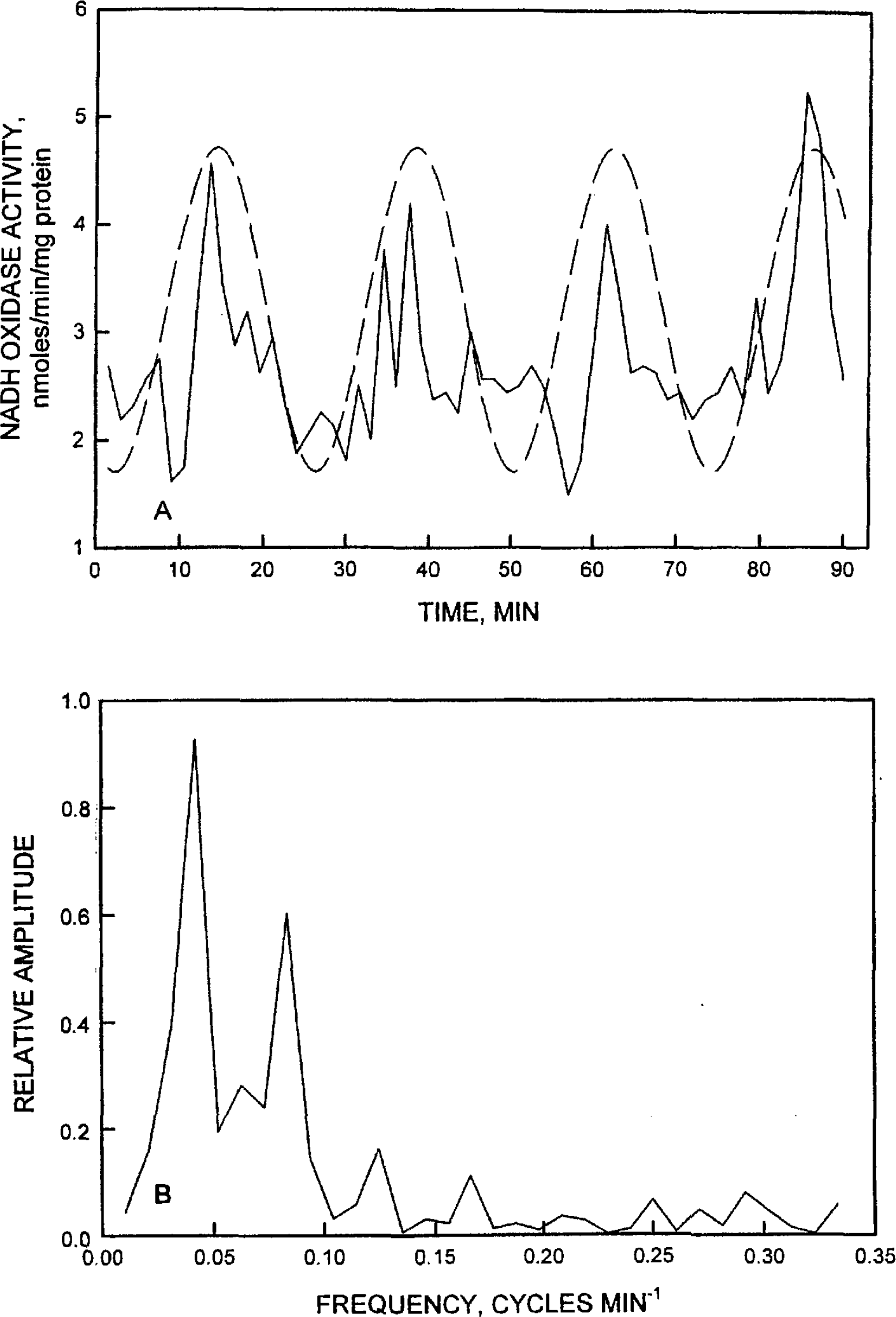
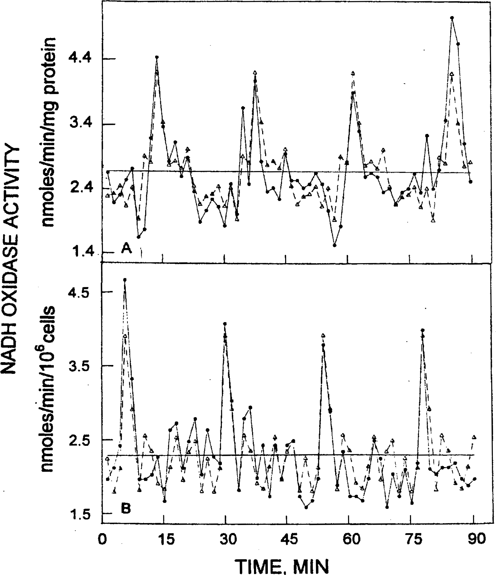
The oscillatory component under investigation is the oxidation of NADH measured as the decrease in A₃₄₀. When represented as rate of NADH oxidation (rate of decrease in A₃₄₀), a dominant period length of ca 24 min was seen clearly as illustrated in Figure 1A for milk fat globule membranes (a derivative of the human or bovine mammary gland epithelium) that had been stored for several months at −70°C. Activity maxima and minima alternated with a period length of 24 min. Means at maxima and minima were different statistically from four parallel determinations (p < 0.001). These data were fitted by a sine wave (Figure 2A) and the corresponding Fourier analysis (Figure 2B) of the oscillations of Figure 2A verified that the oscillations were periodic (Bloomfield 1976). The determined frequency was 0.042 cycles min⁻¹ or a period of 23.8 min.

Figure 1.

Periodicity of NADH oxidase activity as a function of time over 90 min. (A) Intact globule membranes from human milk with maxima in rate of NADH oxidation at ca 24-min intervals beginning at 13.5 min (maxima at 13.5, 37.5, 61.5, and 85.5 min). (B) WI-38 cells with maxima at ca 24-min intervals beginning at 6 min (maxima at 6, 30, 54, and 78 min). Asterisks indicate maxima and minima tested for statistical significance (p < 0.001). Results are from four parallel determinations of the rate of NADH oxidation with time. Each of two determinations were carried out simultaneously using two side-by-side Hitachi U3210 spectrophotometers. Rates of NADH oxidation were measured over 1 min at intervals of 1.5 min. Simultaneous determinations permit direct averaging without need for phasing. A second pair of determinations, phased to be in synchrony with the first pair of determinations, was then carried out. Results are means of the 4 determinations + standard deviations.

Figure 2.

Sine function and Fourier analysis of data of Figure 1A for the human milk fat globule membranes. (A) A sine function was fitted to the data (dotted curve) according to the equation t = 0.25 + 0.1 sin (16 π t/180 + 160 π/180) where t = time in min and the value of 0.25 is the mean rate of decrease in A₃₄₀. (B) The maximum amplitude for Fourier analysis coincided with a frequency of 0.042 cycles/min and corresponded to a period length of 23.8 min.

For the oscillatory behavior to be observed does not require that the cell surface NADH oxidase protein be associated with membranes. Oscillations of 24 min were observed with milk fat globule membranes after the membranes had been solubilized and the integrity of the membrane had been disrupted by treatment with 1% Triton X-100 (not illustrated).

With the reagents alone (no enzyme source) or the enzyme plus all reactants but lacking NADH, no periodic fluctuations were observed. Several different spectrophotometers were compared with similar results.

A second example is provided by the oscillatory pattern of NADH oxidation exhibited by intact WI-38 cells (Figure 1B). The maxima and minima alternate with a period length of ca 24 min and differences among maxima and minima were statistically significant (p < 0.001). The rate of oxidation of NADH for Figure 1A = 0.25 + 0.1 sin (15.2 π)/180 + 200 71/180) where t = time in min and the value of 0.25 is the mean rate of NADH oxidation determined from the decrease in A₃₄₀, the absorption maxima of NADH. The sine function described by the equation (dashed sine function of Figure 3A) approximated the experimentally determined values. Similarly for Figure 1B, the rate of oxidation of NADH was ≌ 0.25+0.1sin(15.2π t)/180 +200π/180 where t = the time in min and the value of 0.25 is the mean rate of NADH oxidation determined from the decrease in A₃₄₀.

Figure 3.

Sine function and Fourier analysis of data of Figure 1B for WI-38 cells. (A) A sine function was fitted to the data (dotted curve) according to the equation t = 0.25 + 0.1 sin (16 π t/180 + 160 π/180) where t = time in min and the value of 0.25 is the mean rate of decrease in A₃₄₀. (B) The maximum amplitude for Fourier analysis coincided with a frequency of 0.042 cycles/min and corresponded to a period length of 23.8 min.

The decomposition fit analyses, illustrated in Figure 4, were used to validate the periodic pattern. Observations were recorded at 90-s intervals. Consequently, the 24-min cycle involves repetition every 16 observations. This means that the number of seasons S in the additive decomposition analysis was set to 16. The resulting “deseasonalized” data were plotted. Thus, the oscillatory behavior and period length of about 24 min seen in Figure 1 were confirmed as reproducible. In the four experiments carried out in parallel with WI-38 cells on different days beginning at the same time, maxima and minima occurred at regularly spaced intervals of 24 min. Differences between maxima and minima were significant (p < 0.001). However, neither the repetitions nor the Fourier analyses of Figures 2 and 3 evaluated clearly the fine details of the oscillatory patterns. For example, visual examinations of the data of Figure 1A and B reveal a recurrent pattern of five activity maxima within each 24-min period, a statistically significant maximum followed by four lesser maxima. This pattern is especially evident in Figure 1B. The lesser maxima are not statistically different from each other or from intervening minima. However, they do occur in each of the three activity periods represented. The reproducibility of these intervening maxima is illustrated by their recapitulation in the time series analysis of Figure 4.

Figure 4.

Seasonal decomposition analyses of data of Figure 1 . Decomposition fits (open triangles, dotted lines) show the reproducibility of the pattern of periodicity. The trend component is represented as a continuous solid line. (A) Intact fat globule membranes from human milk. Maxima were observed at 13.5, 37.5, 61.5, and 85.5 min. (B) WI-38 cells. Maxima were observed at 6, 30, 54, and 78 min.

Classical decomposition decomposes a time series into a trend, cyclic, and error components. In Figure 4, the trend component has been included. The regression results for the trend were:

T r e n d = 0.26 - 0.001 t

with t-statistics of 20.8 and −3.80, respectively, for the estimated coefficients such that the slope is statistically significant. The measured values of Table 1 evaluate the accuracy of the fitted values and include MAPE (13.0 and 12.4), MAD (0.34 and 0.27), and MSD (0.20 and 0.11). The fitted values by either simple decomposition or by the Holt-Winters seasonal exponential method using additive models, agreed closely with the experimental data.

The R-squared values in Table 1 were constructed by computing the squares of the simple correlation coefficients between the actual and forecasted values. These are analogous to an R-square in the regression context and demonstrate a measure of fit. While they are not particularly large, in all cases, there is a strong positive relationship demonstrated between the actual and predicted values.

The graphs in the figures visually demonstrate that the model generally forecasts the direction of movement of the actual data over time. However, such visual appraisal can be deceiving and the ability to discern it depends somewhat on the scale of the graph.

Table 1 lists the p-values associated with the Henriksson and Merton test for each data series and the decomposition and Holt-Winters models. By this criterion, the model performs exceptionally well with the p-values approaching zero for a reasonable level of precision. There appears to be little benefit from the smoothing procedure based on this test. Finally, Figure 6 displays the deterministic seasonal components from the smooth decomposition analyses. Note that they repeat every 16 observations or every 24 min.

Figure 5.

As in Figure 4, except that the Holt-Winters method of smoothing was used. No trend component was estimated for the Holt-Winters model.

Figure 6.

Estimated seasonal pattern from decomposition analysis.

DISCUSSION

Despite knowledge of a biological clock for many years, there have been no candidate molecules for biochemical oscillators capable of functioning as ultradian timekeepers (Edmunds Jr. 1998). The period length of the oscillations of the NOX protein is an essential feature of any biochemical oscillator suggested to function as an ultradian time keeper (Edmunds Jr. 1998) and is largely unaffected by changes in temperature (temperature compensated) (Kippert and Lloyd 1995).

The oscillations in activity are inherent in the cell surface NADH oxidase protein itself and are not dependent on a more complex environment (Morré and Morré 1998). NOX proteins released from the milk fat globule membrane by detergent exhibited an oscillating NOX activity essentially unchanged from that of the isolated milk fat globule membranes (Morré et al. 2002a). A cloned and expressed NOX from HeLa also exhibited a periodicity unchanged from that of the HeLa plasma membrane (Chueh et al. 2002).

Machine variation and/or cycling of reagent (Morré and Morré 1998) do not explain the periodicity. Blanks lacking NADH or lacking an enzyme source did not exhibit periodicity. Additionally, when solubilized and partially purified preparations from different batches of milk fat globules exhibiting periods displaced by several min were mixed, the mixtures displayed both periods (Morré et al. 2002a). This phenomenon would not be expected if the periodicity were the result of interactions among chemical reactants rather than inherent in the protein molecule itself. Similarly, the 24 min periodic oscillations have been observed with solubilized and extensively purified preparations of the plasma membrane NADH oxidase from a plant source (Morré and Morré 1998) and from whole cells and plasma membranes of CHO (Pogue et al. 2001) and HeLa (Wang et al. 2001) cells and by a cloned form of the activity expressed in bacteria (Chueh et al. 2002). We have measured oxygen consumption in parallel to NADH oxidation and it also oscillates with a 24-min period similar to NADH oxidation.

While the data do not appear to contain a trend component, such a conclusion simply from visual appraisal can be misleading. One of the advantages of decomposition is the uncovering of hidden components such as trends, secondary maxima and cycles. A nonconstant amplitude of the seasonal and/or cyclical components may mask the trend and/or other component.

Decomposition was developed to analyze data collected on observable seasonal and/or cyclical frequencies, e.g., monthly or quarterly, or following other cycles. In our analysis, there was no calendar to track the cyclical component. At the same time, the analyses clearly demonstrated that an oscillatory component existed. While the amplitude of this component may vary, the period length was relatively constant.

Fourier analysis was employed to obtain a precise estimate of the duration of the period. The Fourier model posits a linear relationship between NADH oxidase activity and the sine and cosine of time. This allows a smooth oscillatory function to be superimposed on the data. The period length estimated for the function provides an estimate of the period length for the application of the decomposition method. Clearly, however, the Fourier model is not a precise predictor of NADH oxidase. It fails to allow for discrete shifts according to the position in the period that the observation occupies nor does it embody an error correction feedback to update future forecasts based on past forecast errors. The superposition of a simple sine function on the data may be inappropriate due to the possibility of more complex recurring oscillatory components. That is, there are clearly nonsinusoidal dynamics represented in the data. Thus, our attention turned toward finding a more suitable alternative to analyses of these data by decomposition and exponential smoothing.

In the time series analysis, the deviation from the mean showed a recurrent pattern where values were positively correlated over time (autocorrelated or serially correlated). Decomposition fit analyses and Holt-Winters seasonal exponential smoothing using the additive model also were applied to validate both trend (normally constant, i.e., no slope) and the periodic pattern. The additive method was regarded as more appropriate than the multiplicative method since the periodic pattern was independent of data size (Pinduck and Rubinfeld 1991, Box and Jenkins 1976).

The decomposition fits were very similar to those obtained by the Holt-Winters method (Figures 5 and 6, Table 1). What the analyses revealed was the virtual absence of a trend, that is, the oscillatory behavior did not dampen or fluctuate markedly from one major period to the next. Also revealed was a pattern, with both the milk fat globule membranes and the WI-38 cells, of an activity maximum followed by four minor oscillations all within the 24-min period. The potential validity of the minor oscillations including a pattern of three stronger oscillations, followed by two weaker oscillations with the milk fat globule membrane, become evident only with the decomposition fits. The major source of error when determinations made at different times are phased and averaged of the method may be the result of the necessity of averaging rates over 1 min at 1.5-min intervals such that rates from one determination to the next are not made precisely at maxima or minima, especially since the four minor oscillations appear unequally spaced within the 24-min major period.

While the potential complexity of the oscillatory pattern revealed by decomposition was unexpected, the principal value rests in the validation of the oscillatory nature of the response with a period length of about 24 min. From that standpoint, seasonal decomposition analysis emerges as a tool with potentially useful applications to the evaluation of complex biological rhythms.

Current clock models suggests the operation of feedback loops. Time delays in protein translation and transcriptional transport back to the nucleus are thought to cause activities to fluctuate as a function of the light-dark cycle (Konopka and Benzer 1971; Young 2000). While feedback loops may seem essential to the construction of a true 24-h time-keeping system capable of coordination of the many aspects of cell function under circadian control (Jin et al. 1999; Kume et al. 1999; Toh et al. 2001; Lee et al. 2001; Dunlap 1999; Panda et al. 2002), they may not be the actual clock drivers. Organisms that carry mutations in the postulated time-keeping genes retain aspects of circadian control. The operation of feedback loop genes at all times in all cells of all organisms that exhibit circadian rhythms remains to be established (Jin et al. 1999; Kume et al. 1999; Toh et al. 2001). In contrast, the ECTO-NOX proteins appear as universal cell constituents that keep time over widely varying conditions and without interruption.

There is a growing body of evidence to relate redox properties to circadian rhythms. The clock-related transcription factors, NPAS1 and Clock, are intracellular redox sensors (Konopka and Benzer 1971). DNA binding activities of NPAS2 and Clock are influenced by the redox status of NAD(H) and/or NADP(H) (Rutter et al. 2001). Because NOX proteins function as terminal electron acceptors of plasma membrane electron transport (I), their activities provide a significant mechanism for regeneration of cytosolic NAD(P)⁺ from NAD(P)H (Larm et al. 1994). Additionally, respiratory oscillations in continuous yeast cultures are dictated by the demands of a temperature-compensated ultradian clock with a period of about 50 min (Lloyd et al. 2002). However, electron transport components (NADH and cytochromes c and c oxidase) that show redox state changes as the organisms oscillate between their energized and de-energized phases may not be part of the clock mechanism per se but a response to an energetic requirement.

Footnotes

ACKNOWLEDGMENTS

The work was supported by NASA.

References

Bloomfield

. 1976. Fourier Analysis of Time Series: An Introduction. John Wiley & Sons, New York

Box

GEP

and Jenkins

. 1976. Time Series Analyses. Forecasting and Control. Holden-Day, San Francisco

Brightman

Barr

Crane

and Morré

. 1988. Auxin-stimulated NADH oxidase purified from plasma membrane of soybean. Plant Physiol 86:1264–1269

Brightman

Wang

Miu

Sun

Barr

Crane

and Morré

. 1992. A growth factor- and hormone-stimulated NADH oxidase from rat liver plasma membrane. Biochim Biophys Acta 1105:109–117

Bruno

Brightman

Lawrence

Werderitsh

Morré

and Morré

. 1992. Stimulation of NADH oxidase activity by growth factors and hormones is decrease or absent with hepatoma plasma membranes. Biochem J 284:625–628

Chueh

P-J

Morré

Penel

DeHahn

and Morré

. 1997. The hormone-responsive NADH oxidase of the plant plasma membrane has properties of a NADH: protein disulfide reductase. J Biol Chem 272:11221–11227

Chueh

Kim

Cho

Tang

Morré

and Morré

. 2002. Molecular cloning and protein expression of a unique hydroquinone (NADH) oxidase (tNOX) of the cancer cell surface. Biochemistry 41:3732–3741

Dickey

and Fuller

. 1979. Distribution of the Estimators for Autoregressive Time Series with a Unit Root. J American Stat Assoc 74:427–431

Dunlap

. 1999. Molecular bases for circadian clocks. Cell 96:271–290

10.

Edmunds

Jr . 1998. Cellular and Molecular Basis of Biological Clocks. Springer-Verlag, New York, Berlin, Heidelberg

11.

Enright

. 1965. The search for rhythmicity in biological time-series. J Theoret Biol 8:426–468

12.

Foster

and Havenner

. 1999. Cointegration and settlement of commodity futures contracts. Macroeconomic Dynamics 3:226–242.

13.

Fuller

. 1985. Nonstationary Autoregressive Time Series. In: Hannan

Krishnaiah

Rao

, (eds), Time Series in the Time Domain, North Holland, Amsterdam

14.

Gaynor

and Kirkpatrick

. 1994. Introduction to Time Series Modeling and Forecasting in Business and Economics. McGraw-Hill, Inc, New York

15.

Gilbert

and Joosting

ACC

. 1994. The inverse periodogram: a linearising, inverting modification of norm-analysis. BioSystems 31:191–193

16.

Harvey

. 1993. Forecasting, structural time series and the Kalman Filter. Cambridge University Press, New York

17.

Henriksson

and Merton

. 1981. On market timing and investment performance. II. Statistical procedures for evaluating forecasting skills. J Business 54:513–533

18.

Jin

Shearman

Waver

Zylka

de Vries

and Reppert

. 1999. A molecular mechanism regulating rhythmic output from the suprachiasmatic circadian clock. Cell 96:57–68

19.

Keenan

Morré

and Huang

C-M

. 1974. Membranes of the mammary gland. In: Larson

Smith

, (eds), Lactation. A Comprehensive Treatise, pp 191–233. Academic Press, New York

20.

Kippert

and Lloyd

. 1995. A temperature-compensated ultradian clock ticks in: Schizosaccharomyces pombe . Microbiology 141:883–890

21.

Konopka

and Benzer

. 1971. Clock mutants of Drosophila melanogaster . Proc Natl Acad Sci USA 68:2112–2116

22.

Kume

Zylka

Sriram

Shearman

Waver

Jix

Maywood

Hastings

and Reppert

. 1999. mCRYl and mCRY2 are essential components of the negative limb of the circadian clock feedback loop. Cell 98:193–205

23.

Lambeth

Cheng

Arnold

and Edens

. 2000. Novel homologs of gp91phox. TIBS 25:459–461

24.

Larm

Vaillant

Linnane

and Lawen

. 1994. Upregulation of the plasma membrane oxidoreductase as a prerequisite for the viability of human Namalwa rho O cells. J Biol Chem 269:30097–30100

25.

Lee

Etchegaray

Cagampang

Loudon

and Reppert

. 2001. Posttranslational mechanisms regulate the mammalian circadian clock. Cell 107:855–867

26.

Lloyd

Eshantha

Salgado

Turner

and Murray

. 2002. Respiratory oscillations in yeast: Clock-driven mitochondrial cycles of energization. FEBS Lett 519:41–44

27.

Morré

and Morré

. 1995. Differential response of the NADH oxidase of plasma membranes of rat liver and hepatoma and HeLa cells to thiol reagents. J Bioenerg Biomemb 27:137–144

28.

Morré

Chueh

P-J

and Morré

. 1995a. Capsaicin inhibits preferentially the NADH oxidase and growth of transformed cells in culture. Proc Natl Acad Sci USA 92:1831–1835

29.

Morré

L-Y

and Morré

. 1995b. The antitumor sulfonylurea N-(4-methylphenylsulfonyl)-N-(4-chlorophenyl)urea (LY181984) inhibits NADH oxidase activity of HeLa plasma membranes. Biochim Biophys Acta 1240:11–17

30.

Morré

Brightman

Hidalgo

and Navas

. 1995c. Selective inhibition of auxin-stimulated NADH oxidase activity and elongation growth of soybean hypocotyls by thiol reagents. Plant Phys 107:1285–1291

31.

Morré

Sun

Geilen

L-Y

de Cabo

Krasagakis

Orfanos

and Morré

. 1996. Capsaicin inhibits plasma membrane NADH oxidase and growth of human and mouse melanoma lines. Eur J Cancer 32A: 1995–2003

32.

Morré

Jacobs

Sweeting

de Cabo

and Morré

. 1997. A protein disulfide-thiol interchange activity of HeLa plasma membranes inhibited by the antitumor sulfonylurea N-(4-methylphenylsulfonyl)-N-(4-chlorophenyl) urea (LY181984). Biochim Biophys Acta 1325:117–125

33.

Morré

. 1998. NADH oxidase: A multifunctional ectoprotein of the eukaryotic cell surface. In: Asard

Bérczi

Caubergs

, (Eds.), Plasma Membrane Redox Systems and their Role in Biological Stress and Disease, pp 121–156. Kluewer Academic Publishers, Dordrecht, The Netherlands

34.

Morré

and Morré

. 1998. NADH oxidase activity of soybean plasma membranes oscillates with a temperature compensated period of 24 min. Plant J 16:277–284

35.

Morré

Lawler

Wang

Keenan

and Morré

. 2002a. Entrainment in solution of an oscillating NADH oxidase activity from the bovine milk fat globule membrane with a temperature-compensated period length suggestive of an ultradian time-keeping (clock) function. Biochim Biophys Acta 1559:10–20

36.

Morré

Chueh

P-J

Pletcher

Tang

L-Y

and Morré

. 2002b. Biochemical basis for the biological clock. Biochemistry 41:11941–11945

37.

Panda

Hogenesch

and Kay

. 2002. Circadian rhythms from flies to human. Nature 417:329–335

38.

Phillips

PCB

. 1986. Understanding spurious regressions in econometrics. J of Econometrics 33:311–340

39.

Pinduck

and Rubinfeld

. 1991. Econometric Models and Economic Forecasts, 3rd ed. McGraw-Hill, New York

40.

Pogue

Morré

and Morré

. 2001. CHO cell enlargement oscillates with a temperature-compensated period of 24 min. Biochim Biophys Acta 1498:44–51

41.

Rutter

Reick

and McKnight

. 2001. Regulation of clock and NPAS2 DNA binding by the redox state of NADH cofactors. Science 293:510–514

42.

Smith

Krohn

Hermanson

Mallia

Gartner

Provenzano

Fujimoto

Goeke

Olson

and Klenk

. 1985. Measurement of protein using bicinchoninic acid. Anal Biochem 150:70–76

43.

Toh

Jones

Eide

Hinz

Virshup

Ptacek

and Fu

. 2001. An hPer2 phosphorylation site mutation in familial advanced sleep phase syndrome. Science 291:1040–1043

44.

Wang

Morré

and Morré

. 2001. NADH oxidase activity (NOX) and enlargement of HeLa cells oscillate with two different period lengths of 22 and 24 minutes corresponding to different NOX forms. Biochim Biophys Acta 1539:192–204

45.

Winters

. 1960. Forecasting Sales by Exponentially Weighted Moving Averages. Management Science 6:324–342

46.

Young

. 2000. Life's 24-hour clock: molecular control of circadian rhythms in animal cells. Trends in Biochem Sci 25:601–606

Decomposition Analyses Applied to a Complex Ultradian Biorhythm: The Oscillating NADH Oxidase Activity of Plasma Membranes Having a Potential Time-Keeping (Clock) Function

Abstract

Keywords

INTRODUCTION

MATERIALS AND METHODS

Growth of Cells

Isolation of Milk Fat Globule Membranes

NADH Oxidase Activity

Time Series (Decomposition Fit) Analyses

Holt-Winters Exponential Smoothing

RESULTS

DISCUSSION

Footnotes

ACKNOWLEDGMENTS

References