Abstract
Introduction
Logistic regression analysis is frequently used to estimate the relationships between dichotomized dependent variable and continuous independent variable; however, even an evidence of highly significant relationship could be insufficient for the decision-making. Thorough analysis of event probability growth patterns could be helpful to classify cases and to determine cut-off criterions that could be based on critical points of the graph corresponding to the changes in the velocity of event probability growth per unit of predictive variable. The objective is to study the specific features of logistic regression curves to evaluate those critical points.
Materials and Methods
A total of 15 logistic regression functions estimated during scientific studies were analyzed. Points in the graph that correspond to the changes in velocity of probability growth per unit of predictive variable were estimated using second, third, and fourth derivatives of estimated logistic regression functions. The calculated values were then used for predictive variables corresponding to zero points of derivatives to calculate the respective probability values applying estimated previous logistic regression function. Finally, the structure of logistic regression graphs was analyzed and divided into several parts as shown in Fig. 1.
Results
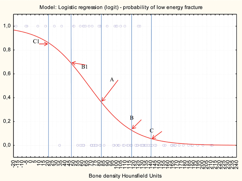
Typical logistic regression curve is shown in Fig. 1.
It was revealed that logistic regression function graphs have the same structure. Point A corresponds to zero point of second derivative, the value of corresponding probability is 0.5. B and B1 points correspond to zero values of third derivative, the values of probability are 0, 21132 and 0, 0.788675, respectively. C and C1 correspond to zero points of fourth derivative and the corresponding probability values are 0.091751 and 0.90824, respectively. Up to point C, there is a baseline of the event with a minor velocity of probability growth. Part of the graph (from point B to C) represents the initial increase in velocity of probability growth, while the one from B to B1 represents maximal velocity of probability growth per unit of predictive variable.
Conclusions
This type of analysis can be applied to decision-making, while it is possible to reveal borders for part of the graph that is indicated as B–C part in Fig. 1. This part of the graph corresponds to the initial acceleration in probability of event growth per unit of predictive variable (e.g., the onset of the disease); consequently, those patients should be put under observation. Further shifts of predictive variable value to the B–B1 part of the graph should be taken under consideration and appropriate treatment should be applied as the velocity of probability growth becomes maximal. The example for this analysis application could be a relationship between low energy vertebra fractures rate and bone density.