Sage Journals: Discover world-class research

Abstract

Higher biologic systems operate far from equilibrium resulting in order, complexity, fluctuation of inherent parameters, and dissipation of energy. According to the decomplexification theory, disease is characterized by a loss of system complexity. We analyzed such complexity in patients after subarachnoid hemorrhage (SAH), by applying the standard technique of variability analysis and the novel method of fractal analysis to middle cerebral artery blood flow velocity (FV) and arterial blood pressure (ABP). In 31 SAH –patients, FV (using transcranial Doppler sonography) and direct ABP were measured. The standard deviations (s.d.) and coefficients of variation (CV = relative s.d.) for FV and ABP time series of length 2¹⁰ secs were calculated as measures of variability. The spectral index β_low and the Hurst coefficient H_bdSWV were analyzed as fractal measures. Outcome was assessed 1 year after SAH according to the Glasgow Outcome Scale (GOS). Both FV (β_low = 2.2±0.4, mean±s.d.) and ABP (β_low = 2.3±0.4) were classified as nonstationary (fractal Brownian motion) signals. FV showed significantly (P <0.05) higher variability (CV = 7.2±2.5%) and Hurst coefficient (H_bdSWV = 0.26±0.13) as compared with ABP (CV = 5.5±2.7%, H_bdSWV = 0.19±0.11). Better outcome (GOS) correlated significantly (P <0.05) with higher s.d. of FV (Spearman's r_s = 0.51, r_s² = 0.26) and ABP (r_s = 0.57, r_s² = 0.32), as well as with a higher Hurst coefficient of ABP (r_s = 0.46, r_s² = 0.21). Cerebral vasospasm reduced CV of FV, but left H_bdSWV unchanged. FV and ABP fluctuated markedly despite homeostatic control. A reduced variability of FV and ABP might indicate a loss of complexity and was associated with a less favorable outcome. Therefore, the decomplexification theory of illness may apply to SAH.

Keywords

arterial blood pressure blood flow velocity fractal analysis Hurst coefficient subarachnoid hemorrhage outcome

Introduction

Homeostasis refers to the ability of the organism to maintain its interior milieu by regulatory mechanisms, as defined by Cannon (1932). It is a property of higher biologic systems, such as the human, and applies to a variety of physiologic parameters, among them cerebral blood flow velocity (FV) and arterial blood pressure (ABP). Both are regulated by an inherent complex system involving interconnected feedback loops. But despite regulation, they are far from being kept constant but rather vary within a certain range. Hence the term ‘stasis’ was considered as somewhat misleading (Seeley and Macklem, 2004), and the concept of homeodynamics (Goodwin, 1997) or – alternatively termed – home-okinesis (Que et al, 2001) has been developed. The latter describes ‘the ability of an organism functioning in a variable external environment to maintain a highly organized internal environment, fluctuating within acceptable limits by dissipating energy in a far-from-equilibrium state’ (Que et al, 2001).

A loss of fluctuation portends increased morbidity and mortality as has been extensively investigated in cardiology: a reduction in heart rate variability is associated with poorer prognosis and/or increased mortality risk in patients with coronary artery disease (Rich et al, 1988), dilated cardiomyopathy (Tuininga et al, 1994), congestive heart failure (Ponikowski et al, 1997), and postinfarction patients (Kleiger et al, 1987).

The pathophysiology of subarachnoid hemorrhage (SAH) has been tried to be understood by identifying individual pathways and determining their interactions. However, a complex system such as the cerebrovascular or the cardiovascular contains more information than the sum of the parts that it consists of (Gallagher and Appenzeller, 1999). We applied an approach, which investigates fluctuations of controlled parameters, seeks a consistent pattern indicative of the presence of a control scheme (Eke et al, 2002) and analyses the complexity of the system itself. Parameters describing such complexity are therefore required, and variability analysis might provide such information (Seeley and Macklem, 2004). Previously, such analysis was performed in the time domain, for instance by analyzing the standard deviation (s.d.) of a time series, or in the frequency domain, for example, by analyzing the power spectral density (PSD) function (Seeley and Macklem, 2004). Lately, with increasing computer power and a deeper understanding on dynamic systems provided by physicists, nonlinear methods such as fractal analysis are performed which are thought to give new insights on the complexity of systems such as the human organism (Bassingthwaighte et al, 1994; Eke et al, 2000).

We hypothesize that variability and fractal analysis of FV and ABP provide useful information regarding the complexity of the human regulatory system when disturbed by SAH. Therefore, we performed this study to investigate the amount of variability of FV and ABP in SAH, to examine the effect of vasospasm on variability, and to analyze the association between variability and patient outcome.

Materials and methods

In this study, data of ABP and FV as obtained from patients after SAH were analyzed retrospectively. Such data were originally gathered and previously published with respect to indices of autoregulation (Soehle et al, 2004a) and critical closing pressure (Soehle et al, 2004b). The monitoring of FV and ABP emerge from standard clinical protocols of the patient's care. Study was performed with approval of the local ethics committee, and consent to publish recorded anonymous data were obtained.

Patients

Thirty-two patients admitted to the Neuro Critical Care Unit of Addenbrooke's Hospital (UK) with a diagnosis of aneurysmal subarachnoid hemorrhage were investigated. Patients were graded on admission according to the World Federation of Neurosurgical Societies as one (n = 4 patients), two (n = 8), three (n = 8), four (n = 7), and five (n = 5).

Patients were treated according to a standard protocol (Whitfield et al, 1996) aiming to maintain cerebral perfusion pressure and to prevent secondary ischemia. Nimodipine was given to all patients and triple-H therapy (Kassel et al, 1982) was performed in case of vasospasm. Aneurysms were clipped surgically, except for two in whom they were coiled endovascularly. Twenty patients were ventilated during the monitoring period.

Monitoring

Left and right middle cerebral artery (MCA) FVs were obtained by bilateral transcranial Doppler (TCD) sonography (Neurogard, 2 MHz, Medasonics, Fremont, CA, USA) with the probes fixed to a headband to avoid dislocation (Soehle et al, 2004a). Arterial blood pressure was measured invasively by a radial artery line. ABP, left and right MCA FVs were recorded simultaneously every other day for 20 mins at a sampling frequency of 50 Hz, and stored on a laptop computer for later offline analysis.

Recordings were visually inspected for artefacts. Only artefact-free data with a length of at least 2¹⁰ secs were included into the study. Thus 91 recordings obtained in 31 patients were finally analyzed using Matlab (R13, The MathWorks) with software written or modified by the authors MS and AP: data were resampled at 1 Hz subsequent to application of a Butterworth low-pass filter with a cutoff frequency of 0.5 Hz. Thus only slow changes in FV and ABP were analyzed, whereas fast changes related to the heartbeat were excluded. Variability of FV and ABP were analyzed using a traditional linear method (variability analysis) as well as a modern nonlinear technique (fractal analysis).

Variation Analysis

For the traditional method, data were tested for normal distribution and variability of data (Figure 1A) was quantified by calculation of the s.d.:

s . d . = \sqrt{\frac{\sum {(x - m)}^{2}}{n - 1}}

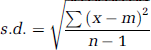
where x denotes the data, m the mean, and n the number of samples. The coefficient of variation (CV= relative s.d.) was calculated as CV=s.d./m and was stated instead of s.d. whenever parameters with different dimensions (e.g., ABP and FV) were to be compared.

Figure 1

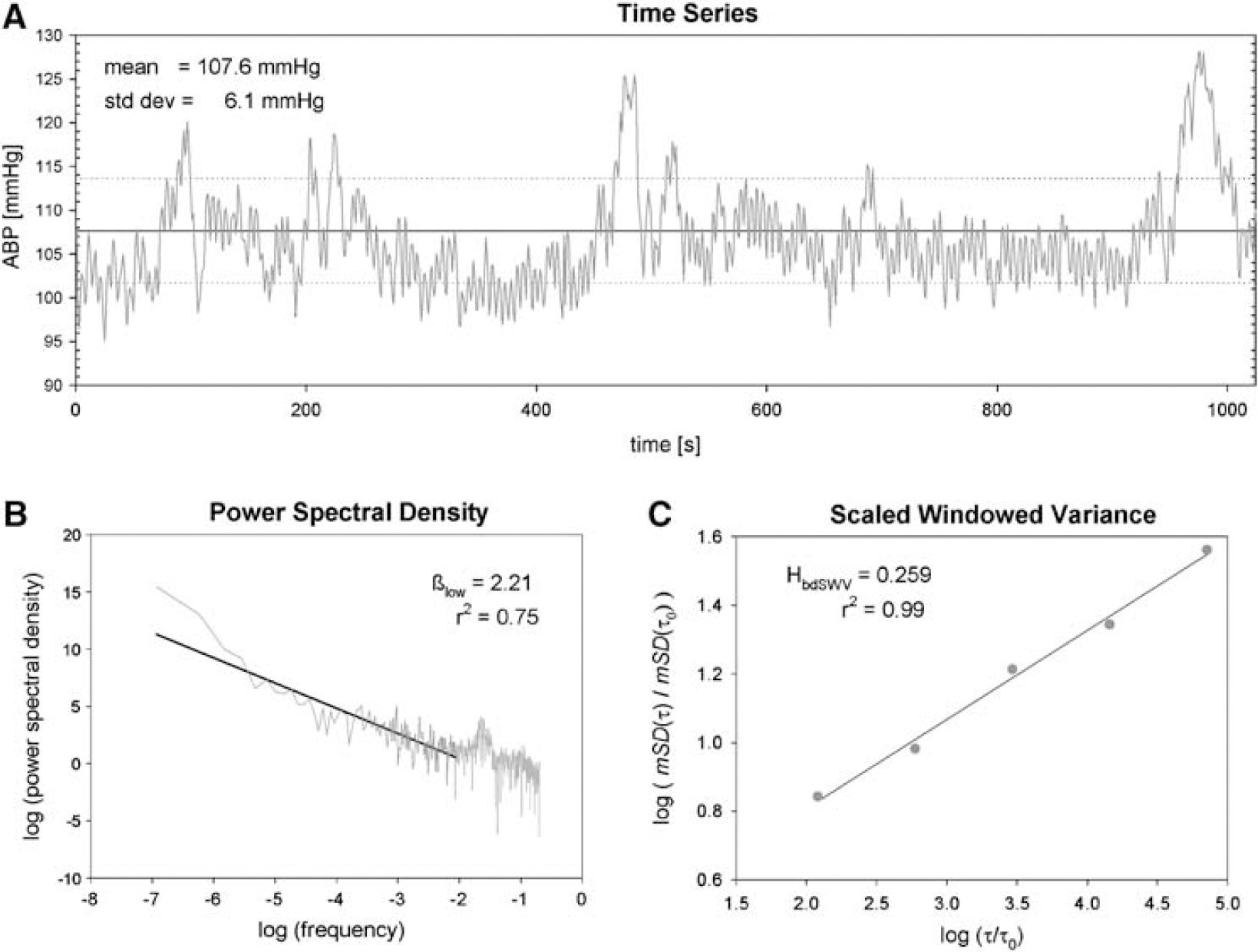
Illustrates the method of variability and fractal analysis as applied to data recorded in a 73-years old female SAH patient: (A) the time series of ABP is shown in the upper part, and mean and s.d. of ABP are indicated by solid and dotted lines, respectively. (B) The power spectral density of ABP as obtained by Fourier analysis is displayed in the left lower part using a log-log scaling. The spectral index β_tow was calculated as the negative slope of the linear regression line, and r as Pearson's correlation coefficient. Only the low frequencies (< 1/8 Hz, shown in dark gray) were considered for regression, whereas the high frequencies (indicated in gray) were excluded. (C) Fractal analysis of ABP as performed by the scaled windowed variance method is presented in the right lower part: the Hurst coefficient H_bdSWV was estimated as the slope of the linear regression of variance (mSD = averaged standard deviation) on time scale τ using a log-log scale.

Fractal Analysis

For the nonlinear method, the data of FV and ABP were regarded as fractal time series. These possess characteristics, one of which is self-similarity: segments of a fractal time series are (geometrically or statistically) similar to larger segments or the whole (Eke et al, 2002). This geometrical or statistical similarity is independent of the time scale chosen, a property known as scale-independence. To quantify the fractal time series, we calculated the Hurst coefficient H (Bassingthwaighte et al, 1994): H gives an estimate of the smoothness of a time series and ranges between 0 and 1, indicating maximal roughness and smoothness, respectively. H was calculated according to the bridge detrended scaled windowed variance (bdSWV) method.

Bridge Detrended Scaled Windowed Variance Analysis

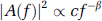
First, the time series was bridge detrended to remove linear trends (Cannon et al, 1997). Then the series was divided into nonoverlapping windows of a reference window size τ₀ = nΔt, and the s.d. of each window was calculated and averaged for that window size τ₀, yielding mSD(τ₀). This computation was repeated for a wide range of window sizes τ. Finally, log[mSD(τ)/mSD(τ₀)] was plotted versus log[τ/τ₀], and the Hurst coefficient H_bdSWV was estimated as the slope of the linear regression line (Cannon et al, 1997; Mandelbrot, 1985) (Figure 1C).

H_{bdSWV} = \frac{log (m S D (τ) / m S D (τ_{0})}{log (τ / τ_{0})}

H_bdSWV is applicable to nonstationary time series only (Eke et al, 2000), which are denoted as fractal Brownian motion (fBm) and which are defined as NOT having constant variation over time. PSD analysis was performed to investigate nonstationarity.

Power Spectral Density Analysis and its Modification PSDlow

Application of the Fourier analysis to a (discrete) time series yields the power spectral amplitude | A(f) |² at frequency f. In fractal time series, | A(f) |² decreases exponentially as frequency f increases, which is known as ‘1/f power law’ (Eke et al, 2002):

| A (f) |^{2} \propto c f^{- β}

where c is a constant and β is the spectral index. β is calculated as the negative slope of the linear regression line of log(| A(f) |²) on log(f) (Figure 1B) and provides information on the signal class of the fractal time series: fractal nonstationary (Brownian motion) time series are having 1 < β < 3, whereas stationary (Gaussian noise) time series are characterized by −1 < β < 1. As suggested by Eke et al (2000), high frequencies above one-eighth of the sampling frequency were excluded before calculation of β, a method referred to as PSD_low, resulting in a spectral index denoted as β_low. In addition, signal summation conversion, that is, conversion of the original time series by taking its cumulative sum, was performed in case of 0.38 < β < 1.04, a range where otherwise classification errors might occur (Eke et al, 2000).

The Matlab code ‘fractool.m’ written by Peter Herman and Andras Eke provides algorithms for calculation of β_low and H_bdSWV. It was slightly modified to fulfill the purposes of this study.

Outcome

Outcome 1 year after SAH was assessed using the Glasgow Outcome Scale (GOS) during a telephone interview by an investigator (DC) who was masked to the ABP and FV data. Three patients were lost during follow-up, six patients were without neurologic deficits (GOS = 5), three were moderately disabled but independent (GOS = 4), 11 were severely disabled and dependent on daily support (GOS = 3), none remained in a persistent vegetative state, and eight patients had died (GOS = 1).

Statistics

To describe the population of the 31 SAH patients, data obtained by variation and fractal analysis were averaged within patients. Parameters were compared between ABP, left and right FVs using one-way analysis of variance, and statistical significance was assumed at a P <0.05.

The effect of cerebral vasospasm on variability and fractal analysis was investigated in 15 patients, who developed vasospasm according to established TCD criteria (mean FV > 120 cm/sec and a Lindegaard ratio >3, (Lindegaard, 1999)). To analyze the temporal effect of vasospasm, parameters obtained before vasospasm were compared with those assessed during vasospasm. Accordingly, values monitored at the side of vasospasm were compared with contralateral values for investigation of the spatial effect of vasospasm.

Correlation between at least interval scaled parameters (e.g., ABP, FV) was performed by application of Pearson's product moment correlation. In case of ordinal-scaled parameters (e.g., GOS), the nonparametric Spearman rank-order correlation was used instead. For both methods the correlation coefficient r (Pearson) or r_s (Spearman), its square (= coefficient of determination) r² (Pearson) or r_s² (Spearman) as a measure describing the strength of the correlation, and its P-value – testing the correlation coefficient to be different from 0 – were stated. All statistical tests were performed using SigmaStat (Jandel Scientific, Erkrath, Germany).

Results

Epidemiology

Thirty-one patients with an age of 50 ± 13 (mean ± s.d.) years fulfilled the inclusion criteria. Their mean data with respect to left and right MCA FVs (87 and 85 cm/sec, respectively) as well as ABP (96 mm Hg) are shown in Table 1.

Table 1

Analysis of MCA FV and ABP

Parameter	Left MCA FV	Right MCA FV	ABP
Mean	86.8 ± 34.0 cm/sec	84.5 ± 35.2 cm/sec	95.7 ± 12.8 mm Hg
Variation analysis
s.d.	5.9 ± 2.6cm/sec	6.1 ± 3.5 cm/sec	5.1 ± 2.4 mm Hg
CV	7.1 ± 2.5%*	7.2 ± 2.1%*	5.5 ± 2.7%
Fractal analysis
Spectral index β_low	2.15 ± 0.37	2.14 ± 0.31	2.30 ± 0.39
Hurst coefficient H_hdSWV	0.26 ± 0.12*	0.26 ± 0.13*	0.19 ± 0.11

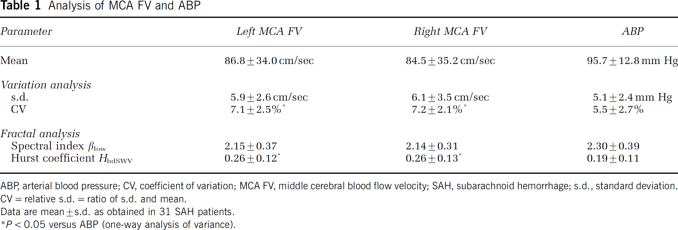
ABP, arterial blood pressure; CV, coefficient of variation; MCA FV, middle cerebral blood flow velocity; SAH, subarachnoid hemorrhage; s.d., standard deviation.

CV = relative s.d. = ratio of s.d. and mean.

Data are mean ± s.d. as obtained in 31 SAH patients.

P < 0.05 versus ABP (one-way analysis of variance).

Variability

A s.d. of 5.9 and 6.1 cm/sec was obtained for the left and right MCA FVs, respectively, and of 5.1 mm Hg for ABP (Table 1). The CV was significantly (P <0.05) higher for left and right MCA FVs (7.1% and 7.2%, respectively) as compared with ABP (5.5%, Table 1). A positive association between the mean and the s.d. was observed in FV (Pearson r =+0.58, r² = 0.34, P < 0.001), but not in ABP (P = 0.99). Examples of patients with low and high variability of ABP and FV time series are shown in Figure 2.

Figure 2

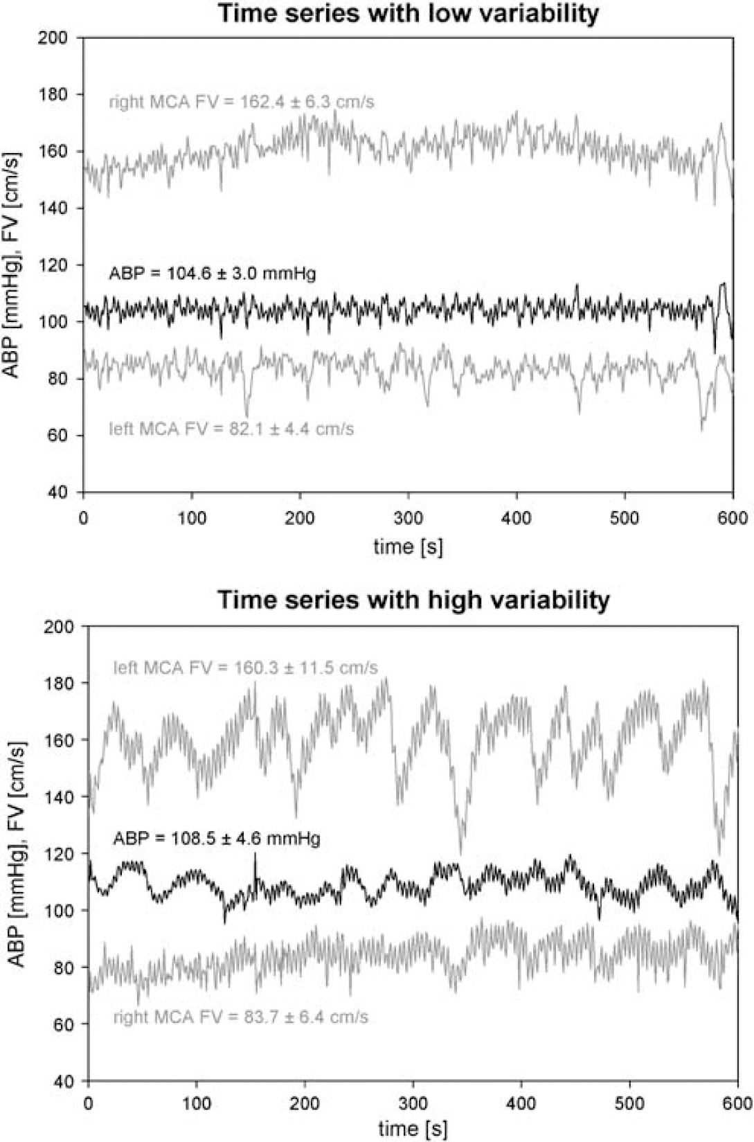
Presents simultaneous recordings of ABP and FV as obtained from the left and right MCA. Time series of patients with low and high variability are shown in the upper and lower part, respectively. Numeric data are given as mean ± s.d.

Fractal Analysis

A spectral index β_low of 2.15 and 2.14 (left and right MCA FVs), and of 2.30 (ABP) was calculated in the 31 patients (Table 1). Of the 91 datasets, 78 ABP, 86 left MCA FV and 89 right MCA FV records were classified as nonstationary (fBm) according to their spectral index. In the remaining files, a second step (signal summation conversion) was required, which classified these data as nonstationary, either. Hence, dSWV was applicable to all recording files. H_bdSWV was significantly (P <0.05) higher for the left and right MCA FVs (0.26 on both sides), as compared with ABP (0.19, Table 1).

Effect of Cerebral Vasospasm

The effect of TCD-defined vasospasm is presented in Table 2. The temporal effect of vasospasm was similar to its spatial effect: cerebral vasospasm was associated with a significant (P <0.05) increase in s.d. and decrease in CV. In addition, the spectral index β_low was significantly elevated by vasospasm, whereas the Hurst coefficient was not affected by it (Table 2). An example how cerebral vasospasm affected the FV time series and its PSD and scaled windowed variance are presented in Figure 3.

Table 2

Temporal and spatial effect of transcranial Doppler-derived cerebral vasospasm on variability and fractal analysis of MCA FV

Parameter	Unit	Before vasospasm	During vasospasm	Contralateral side of vasospasm	Ipsilateral side of vasospasm
Mean FV	cm/sec	74 ± 21	148 ± 18*	81.4 ± 18.3	154.2 ± 20.9#
Variation analysis
s.d.	cm/sec	5.0 ± 2.7	8.1 ± 3.3*	6.9 ± 5.6	10.4 ± 6.5#
CV	%	6.8 ± 2.7	5.5 ± 2.1*	8.4 ± 5.4	6.7 ± 4.0#
Fractal analysis
Spectral index β_low		1.97 ± 0.35	2.23 ± 0.43*	2.09 ± 0.56	2.29 ± 0.61#
Hurst coefficient H_bdSWV		0.24 ± 0.11	0.21 ± 0.13^NS	0.22 ± 0.11	0.23 ± 0.13^NS

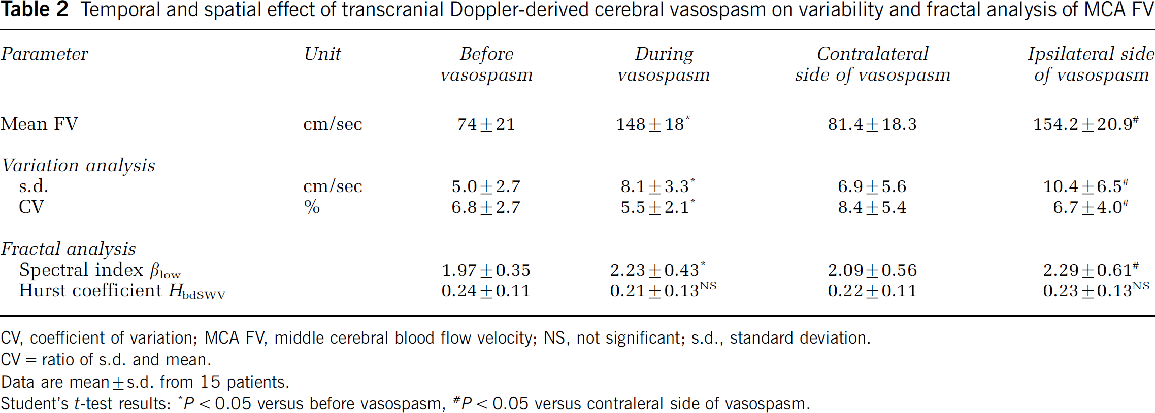
CV, coefficient of variation; MCA FV, middle cerebral blood flow velocity; NS, not significant; s.d., standard deviation.

CV= ratio of s.d. and mean.

Data are mean±s.d. from 15 patients.

Student's t-test results

P < 0.05 versus before vasospasm

P < 0.05 versus contraleral side of vasospasm.

Figure 3

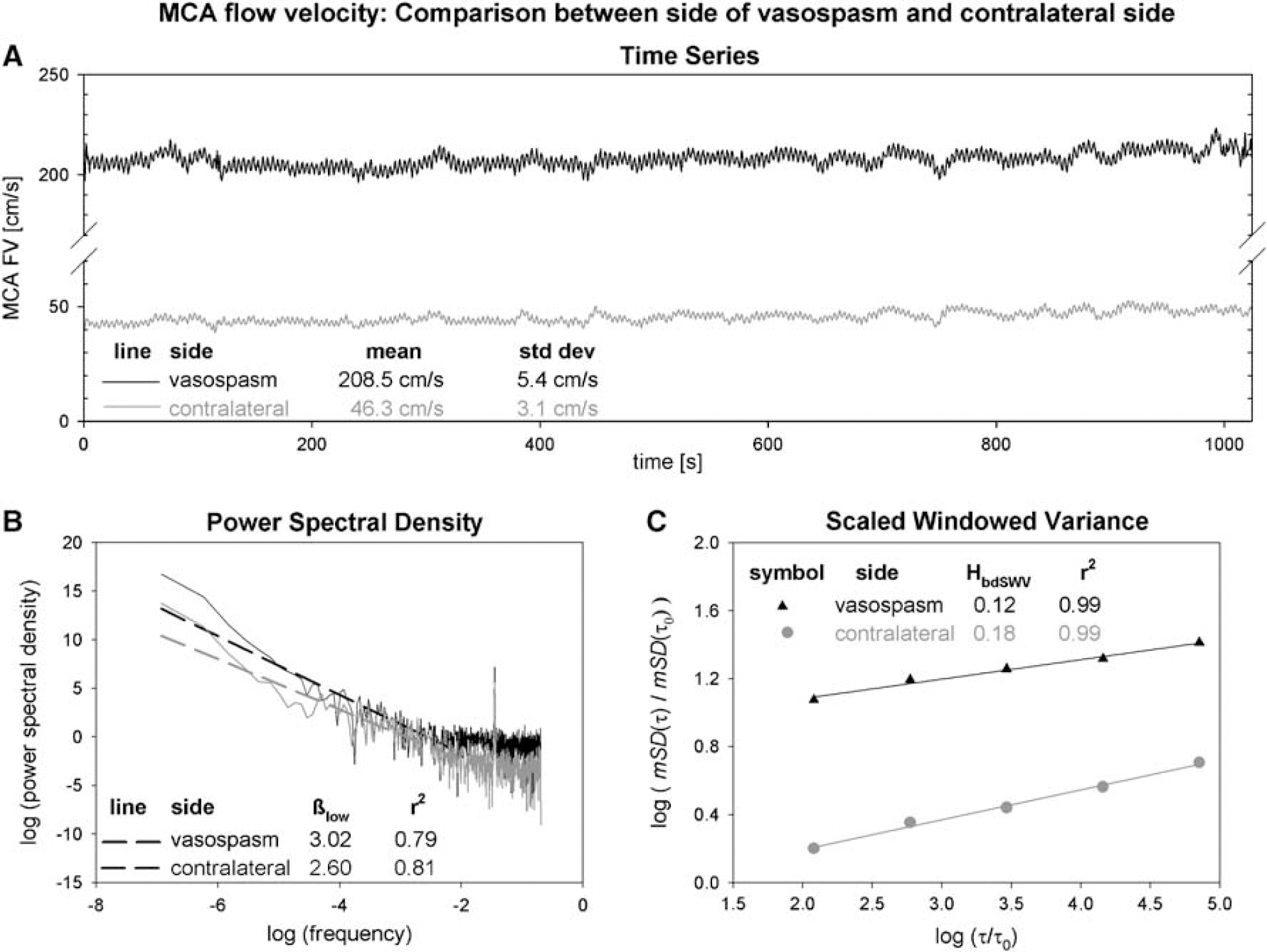
Shows the time series (A) of the MCA FV in comparison between the side of vasospasm (indicated in black) and the contralateral side (indicated in gray). (B) Illustrates the PSD analysis of the time series shown in (A): the spectral index β_low was calculated as the negative slope of the regression line (shown as slashed line) of PSD on frequency at a log-log scale. Note that only frequencies below 1/8 Hz (−2.08 on a log scale) were taken into account. The Hurst coefficient H_bdSWV of the time series shown in (A) was calculated as presented in (C): the averaged standard deviation (mSD) of the time series was plotted versus its time scale (τ) on a log-log scale, and H_bdSWV was estimated as the slope of the regression line. In (B) and (C), r² denotes the square of Pearson's correlation coefficient.

Correlation with Outcome

A high GOS, that is a more favorable outcome, correlated significantly (P <0.05), with a high s.d. of left MCA FV (Spearman r_s = 0.47, r_s² = 0.22, Table 3, Figure 4), right MCA FV (r_s = 0.56, r_s² = 0.31), and ABP (r_s = 0.57, r_s² = 0.32), as well as with a high Hurst coefficient of ABP (r_s = 0.46, r_s² = 0.21).

Table 3

Correlation of MCA FV and ABP with GOS as assessed 1 year after SAH in 28 patients

Parameter	Left MCA FV	Right MCA FV	ABP
Mean
r_s			−0.42
r_s²			0.18
P	NS	NS	0.026
Variation analysis
s.d.
r_s	+0.47	+0.56	+0.57
r_s²	0.22	0.31	0.32
P	0.012	0.002	0.002
Fractal analysis
Hurst coefficient H_bdSWV
r_s			+0.46
r_s²			0.21
P	NS	NS	0.014

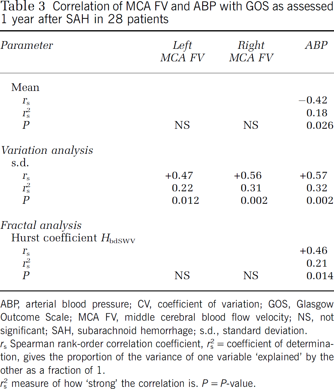
ABP, arterial blood pressure; CV, coefficient of variation; GOS, Glasgow Outcome Scale; MCA FV, middle cerebral blood flow velocity; NS, not significant; SAH, subarachnoid hemorrhage; s.d., standard deviation. r_s Spearman rank-order correlation coefficient.

r_s² = coefficient of determination, gives the proportion of the variance of one variable ‘explained’ by the other as a fraction of 1.

r_s² measure of how ‘strong’ the correlation is. P = P-value.

Figure 4

Illustrates the correlation of four parameters with the GOS, as assessed 1 year after SAH in 28 patients. The parameters are the s.d. of the left MCA FV_MCA (left upper part), right FV_MCA (left lower part), ABP (right upper part), and the Hurst coefficient (H_bdSWV) of ABP (right lower part). The GOS ranges between 1 (death) and 5 (good recovery). Data obtained in patients who developed cerebral vasospasm are shown as black triangles (▲) in contrast to those who did not (○). Spearman rank-order correlation coefficient r_s is given with its respective P-value.

Discussion

Signal Processing

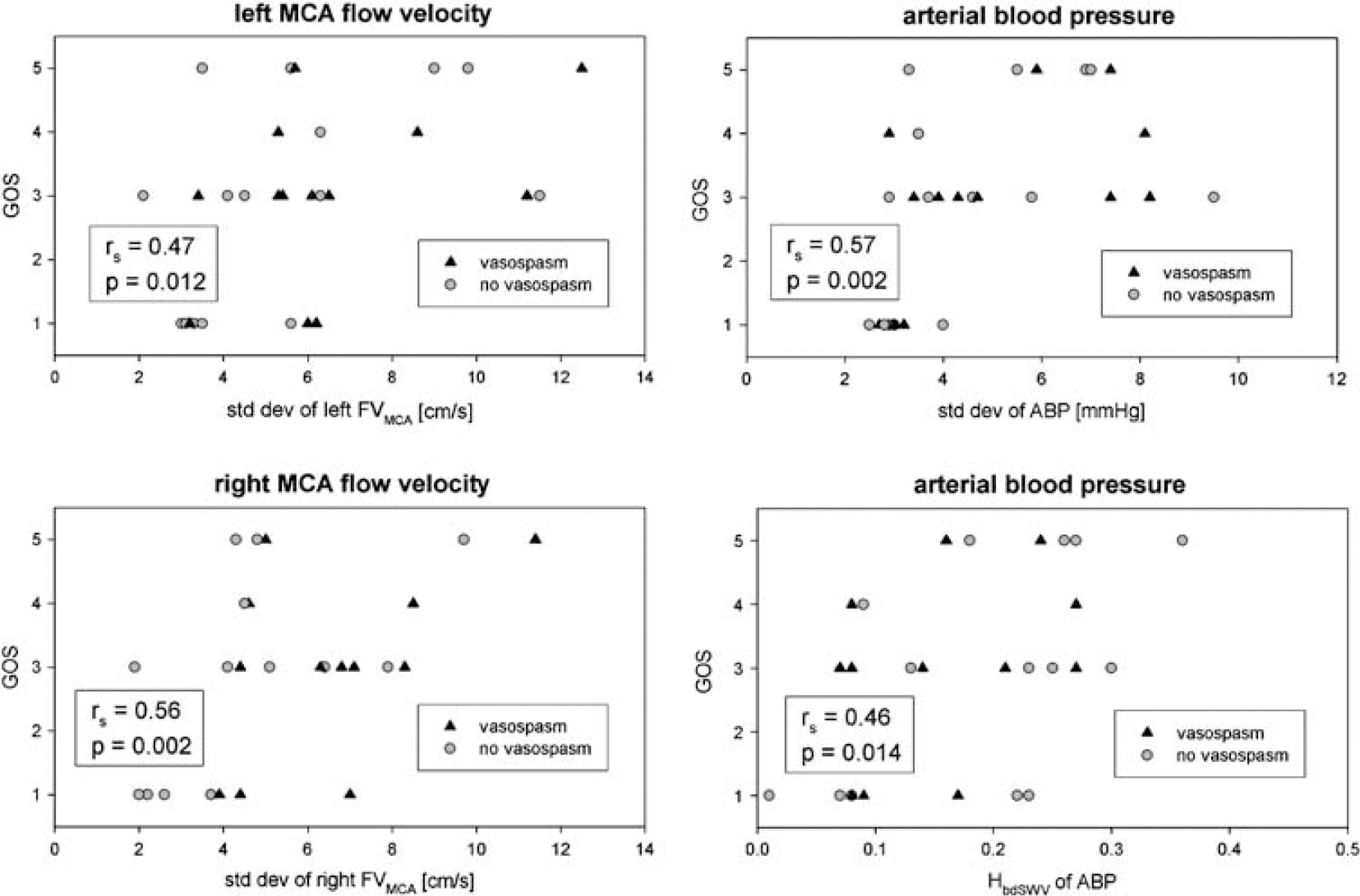
The time series of ABP and FV were originally sampled at 50 Hz and showed periodic, heartbeat-related changes (Figure 5, upper part). Fourier analysis revealed two separate modalities (Figure 5, lower part): In the lower frequency range, amplitudes complied with the 1/f power law as expected from a fractal process, whereas in the higher frequency range (> 1 Hz), amplitudes were dominated by the heartbeat (60 to 120 min⁻¹ = 1 to 2 Hz, corresponding to 0 to 0.69 on a logarithmic scale) and its higher harmonics. Such different modalities within a signal as well as amplitudes dominated by a fractal pattern in the low-frequency range were previously described for cerebral blood volume (Eke et al, 2006). To exclude the periodic, heartbeat-related contents, we resampled the signals at 1 Hz (Figure 5, upper part). To prevent aliasing, time series were low-pass filtered with a cutoff frequency of 0.5 Hz before resampling.

Figure 5

Shows the time series (upper part) of the FV as obtained in the left MCA of a patient after SAH. The 50 Hz sampled original time series (shown in gray) shows the heartbeat-related fluctuations in FV, which were not present in the 1 Hz resampled time series (indicated in black). The power spectrum of the FV time series consisted of two modalities, as shown in the lower part: the higher frequencies (shown in gray on a white background) are dominated by the heart rate (89 min⁻¹) and its higher harmonics (178 and 267 min⁻¹), resulting in the PSD peaks at log(frequencies) of 0.39, 1.09, and 1.49, respectively. The lower frequencies (shown in black on a gray background), followed the 1/f power law characteristic for a fractal process. Resampling at 1 Hz resulted in the power spectrum presented in black on a gray background: The higher frequencies (white background) and especially heartbeat-related changes were eliminated due to resampling. The small PSD peak at a log(frequency)of-1.15 (= 19 min⁻¹) was due to mechanical ventilation.

Mechanical ventilation with a fixed rate (8 to 16 min⁻¹ = 0.13 to 0.26 Hz, corresponding to −2.01 to −1.32 on a logarithmic scale) might induce periodic changes in ABP and FV. Such changes in ABP are pronounced in hypovolemic patients but were minimal in our patients, in which therapy aimed at maintaining normovolemia or even hypervolemia in case of vasospasm. ABP-induced slow changes in FV were further reduced by cerebral autoregulation, at least in cases in which it was preserved. Hence, ventilation-induced fluctuations contributed little to the power of the entire signal. Moreover, frequencies above one-eighth of the sampling frequency (1/8 × 1 Hz = 0.125 Hz) were excluded in PSD analysis as suggested by (Eke et al, 2000), and the smallest two time scales were ignored in bdSWV analysis.

Variability Analysis

Fluctuations of homeostatic controlled parameters are common and have been reported for heart rate (Kleiger et al, 1987), blood pressure (Wagner and Persson, 1995), respiratory rate (Bruce, 1996), tidal volume, and other ventilatory parameters (Suki, 2002). Analysis of such variability provides a novel technology to evaluate the overall properties of a complex system (Seeley and Macklem, 2004). To our knowledge, this is the first study performing variability and fractal analysis in SAH. We observed a considerable amount of variability in both FV and ABP. In addition, variability was more pronounced in FV than in ABP which can be explained by the fact that FV is not only affected by ABP, but by cerebral autoregulation (Soehle et al, 2004a) and ICP as well.

Fractal Analysis

Fractal characteristics are common in biology and physiology, and have been shown in heart rate variability (Ho et al, 1997; Kleiger et al, 1987) and gait dynamics (Hausdorff et al, 2001), for instance. In PSD analysis, both FV and ABP time series followed the ‘1/f power law’ for more than two decades of frequencies (Figures 1B and 3B) and thus fulfilled the criterion of scale invariance, which is a typical property of a fractal time series (Eke et al, 2000). Flow velocity and ABP were classified as fractal Brownian motion by their spectral index β_low and in case of uncertainty by signal summation conversion as suggested by the dichotomous fractal Gaussian noise/Brownian motion model proposed by Eke et al (2000). They reported the same signal class for cerebral FV, however, measured in the rat cerebral microcirculation, whereas we assessed the human cerebral macrocirculation.

We applied bdSWV to estimate H, which is a robust method yielding accurate estimates, however, applicable to fBm time series only (Eke et al, 2002). We thus obtained a H_bdSWV of 0.26 ± 0.13 in the MCA, which is similar to the value of H_bdSWV of 0.24 ± 0.02 reported in the rat cerebral microcirculation (Eke et al, 2000). In contrast, Rossitti and Stephensen (1994) reported a markedly higher H of 0.76 ± 0.09 for human MCA FV in healthy volunteers. However, they applied dispersional analysis (Bassingthwaighte, 1988) for the estimation of H without analyzing for the appropriate signal class, presumably resulting in a wrong classification of the signal as fGn and overestimation of H (Eke et al, 2000). In fact, misclassification of our signal as fGn would have resulted in a H_Disp of approximately 0.78, similar to their result.

For ABP, we obtained a β_low of 2.30 ± 0.39 in SAH –patients, which is close to a spectral index of 2.46 ± 0.13 in healthy volunteers as reported by Blaber et al (1997), using a slightly different methodology.

Physiologic signals are generally nonstationary (Eke et al, 2002), hence their statistical properties change with time. In fact, both FV and ABP were classified as such in our study. The Hurst coefficient of both was unequal to 0.5, which means that the variations in FV and ABP are not random. In addition, it indicates the presence of correlation (or anticorrelation) within both signals: increases of the signal in the past influence increases (in case of correlation) or decreases (in case of anticorrelation) at present. Hence, a long-term memory (Bassingthwaighte et al, 1994; Eke et al, 2002) was present for both FV and ABP.

Variability and fractal analysis provide complementary information regarding signal characteristics (Seeley and Macklem, 2004): s.d. evaluates the overall short-term variation in stationary time series. Despite the nonstationarity of physiologic signals (Eke et al, 2002), s.d. has been proven clinically useful in identifying alterations of signal characteristics (Seeley and Macklem, 2004). BdSWV detects long-range correlations and has been designed for application in nonstationary time series, although being based on s.d. (Eke et al, 2002). Whereas the novel technique of bdSWV analyses s.d. over a wide range of time scales, the classical method of variation analysis investigates s.d. on a single time scale only. Finally, H quantifies the roughness of the signal on a time-invariant scale (Bassingthwaighte et al, 1994).

Effect of Cerebral Vasospasm

In cerebral vasospasm, we observed an increase in s.d. of FV which is likely to be an epiphenomenon of the increased mean FV, by which vasospasm was defined, as shown by the correlation between mean and s.d. of FV. Hence, FV showed a similar behavior to a random variable, in which the s.d. tends to increase as the mean rises. Under such circumstances, the standardized CV is a more appropriate measure of variability: CV was reduced in vasospasm, suggesting a loss of variability. In vasospasm, neither the signal class – which remained nonstationary (fBm) – nor the Hurst coefficient of FV was significantly affected.

Cerebral vasospasm is characterized as a narrowing of cerebral arteries subsequent to SAH. So far, neither the term ‘vasospasm’ nor its diagnosis has been standardized: its diagnosis is either based on a reduction of arterial diameter on cerebral angiogram (angiographic vasospasm), or on an increase in FV (transcranial Doppler-derived vasospasm), or on the occurrence of a new focal neurologic deficit, also known as delayed ischemic neurologic deficit (symptomatic vasospasm).

It should be noted that our results were obtained using a definition of cerebral vasospasm based on transcranial Doppler criteria. Transcranial Doppler and angiographic vasospasms are closely related especially in the MCA (Lysakowski et al, 2001), however, frequently occur without neurologic deficits. Therefore our results might not be applicable to symptomatic vasospasm, which was not investigated in our study, because delayed ischemic neurologic deficits would have happened unrecognized in the majority of our patients because they were ventilated and sedated.

Association with Outcome

Decreased heart rate variability is associated with poorer prognosis in patients with coronary artery disease (Rich et al, 1988), dilated cardiomyopathy (Tuininga et al, 1994), congestive heart failure (Ponikowski et al, 1997), and myocardial infarction (Kleiger et al, 1987). Similarly, we found a reduced variability of ABP and FV and a diminished Hurst coefficient of ABP to be associated with a poorer outcome.

The ‘strength’ of this association was quantified by the coefficient of determination r_s² (Table 3): accordingly, between 21% (H_bdSWV of ABP) and 32% (s.d. of ABP) of the variation in GOS is explained by the variation of the analyzed variability and fractal parameters. Such relatively low coefficients of determination might suggest a rather weak correlation with outcome, but are well within the range reported for established predictors of outcome in SAH, such as age, initial clinical status according to Hunt and Hess, World Federation of Neurosurgical Societies or GOS, and amount of blood on computed tomography (Hutter et al, 2001; Kassel et al, 1990; Koivisto et al, 2000).

Gotoh et al (1996) reported an r_s² of 0.38 for the correlation between Glasgow Coma Scale and GOS, and Chiang et al (2000) calculated an r_s² of 0.09 for age, 0.16 for Hunt and Hess Score, 0.16 for World Federation of Neurosurgical Societies Score, and 0.36 for Glasgow Coma Scale when correlating with GOS.

The correlation with outcome found in our study indicates that variability and fractal parameters seem to contain clinical relevant information. However, it has not been the aim of this study to establish such parameters as outcome predictors. Whether variability and fractal parameters are independent predictors of outcome in SAH, remains to be analyzed in a study including a much larger number of patients.

Interpretation of Altered Variability

In a biologic system working in the state of thermodynamic equilibrium, parameters remain constant without consumption of external energy sources. However, complexity evolves in self-organizing systems that work far from equilibrium (Que et al, 2001). Parameters fluctuate and a continuous source of external energy is required. ‘Normal’ variation is thought to signify adaptability, complexity, and health (Seeley and Macklem, 2004). In contrast, a decreased variability represents ‘decomplexification’ and illness according to Goldberger (1997), as has been shown in Cheyne-Stokes respiration, Parkinsonian gait, neutrophil count in leukemia, and fever in Hodgkin's disease. In accordance, we found a decreased variability in cerebral vasospasm and an association between reduced fluctuation and unfavorable outcome in SAH. In contrast, an increased variability has been described by Vaillancourt and Newell (2002) in acromegaly and Cushing's disease as well as by Que et al (2001) in asthma. It is thus hypothesized that disease is characterized by both excessive and too little variation (Que et al, 2001).

Limitations

Our study is limited by the small number of patients included (n = 31) and of patients who developed cerebral vaospasm (n = 15). Therefore we consider the association found between outcome on the one hand and variability and Hurst coefficient on the other hand as to be confirmed in a larger population of SAH patients: variability and Hurst coefficient should not be regarded as predictors of outcome until they are confirmed by regression analysis.

Another limitation refers to the length of the time series analyzed. In a previous study, we found 2¹⁰ data to yield sufficient estimates of β_low and H_bdSWV with respect to clinical studies. Nevertheless, accuracy of fractal analysis improves with the length of the time series (Eke et al, 2002), but nursing, diagnostic, and therapeutic procedures limited the monitoring period in patients.

Conclusions

We conclude that a considerable amount of fluctuation was present in both FV and ABP after SAH. Variability and fractal analysis provide valuable information regarding the complexity of the human organism: fluctuations are reduced in cerebral vasospasm, and a decrease in variability suggesting a loss of complexity was associated with a less favourble outcome. The decomplexification theory of illness therefore may apply to SAH too.

Footnotes

Acknowledgements

We gratefully acknowledge the provision of the software source codes of ‘fractal.m’ at by Peter Herman and Andras Eke, University of Budapest, Hungary.

Disclosure

The authors declare no financial interest related to the materials and methods presented here.

References

Bassingthwaighte

Liebovitch

West

(1994) Fractal measures of heterogeneity and correlation. In: Bassingthwaighte

Liebovitch

West

(eds). 73 Fractal Physiology. Oxford: Oxford University Press pp. 63–107

Bassingthwaighte

(1988) Physiological heterogeneity: fractals link determinism and randomness in structures and function. News Physiol Sci 3:5–10

Blaber

Bondar

Stein

Dunphy

Moradshahi

Kassam

Freeman

(1997) Complexity of middle cerebral artery blood flow velocity: effects of tilt and autonomic failure. Am J Physiol 273:H2209–16

Bruce

(1996) Temporal variations in the pattern of breathing. J Appl Physiol 80:1079–87

Cannon

Percival

Caccia

Raymond

Bassingthwaighte

(1997) Evaluating scaled window variance methods for estimating the Hurst coefficient of time series. Physica A 241:606–26

Cannon

(1932) The Wisdom of the Body. New York: W.W. Norton

Chiang

VLS

Claus

Awad

(2000) Toward more rational prediction of outcome in patients with high-grade subarachnoid hemorrhage. Neurosurgery 46:28–36

Eke

Herman

Bassingthwaighte

Raymond

Percival

Cannon

Balla

Ikrenyi

(2000) Physiological time series: distinguishing fractal noises from motions. Eur J Physiol 439:403–15

Eke

Herman

Hajnal

(2006) Fractal and noisy CBV dynamics in humans: influence of age and gender. J Cereb Blood Flow Metab 26:891–8

10.

Eke

Herman

Kocsis

Kozak

(2002) Fractal characterization of complexity in temporal physiological signals. Physiol Meas 23:R1–38

11.

Gallagher

Appenzeller

(1999) Beyond reductionism. Science 284:79

12.

Goldberger

(1997) Fractal variability versus pathologic periodicity: complexity loss and stereotypy in disease. Perspect Biol Med 40:543–61

13.

Goodwin

(1997) Temporal organisation and disorganisation in organisms. Chronobiol Int 14:531–6

14.

Gotoh

Tamura

Yasui

Suzuki

Hadeishi

Sano

(1996) Glasgow coma scale in the prediction of outcome after early aneurysm surgery. Neurosurgery 39:19–25

15.

Hausdorff

Ashkenazy

Peng

Ivanov

Stanley

Goldberger

(2001) When human walking becomes random walking: fractal analysis and modeling of gait rhythm fluctuations. Physica A 302:138–47

16.

Moody

Peng

Mietus

Larson

Levy

Goldberger

(1997) Predicting survival in heart failure case and control subjects by use of fully automated methods for deriving non-linear and conventional indices of heart rate dynamics. Circulation 96:842–8

17.

Hutter

Hreitschmann-Andermahr

Gilsbach

(2001) Health-related quality of life after aneurysmal subarachnoid hemorrhage: impacts of bleeding severity, computerized tomography findings, vasospasm, and neurological grade. J Neurosurg 94:241–51

18.

Kassel

Peerless

Durward

Beck

Drake

Adams

(1982) Treatment of ischemic deficits from vasospasm with intravascular volume expansion and induced arterial hypertension. Neurosurgery 11:337–43

19.

Kassel

Torner

Haley

Jane

Adams

Kongable

(1990) The international cooperative study on the timing of aneurysm surgery. Part 1: overall management results. J Neurosurg 73:18–36

20.

Kleiger

Miller

Bigger

Moss

(1987) Decreased heart rate variability and its association with increased mortality after acute myocardial infarction. Am J Cardiol 59:256–62

21.

Koivisto

Vanninen

Hurskainen

Saari

Hernesniemi

Vapalahti

(2000) Outcomes of early endovascular versus surgical treatment of ruptured cerebral aneurysms. A prospective randomized study. Stroke 31:2369–77

22.

Lindegaard

(1999) The role of transcranial Doppler in the management of patients with subarachnoid haemorrhage – a review. Acta Neurochir Suppl (Wien) 72:59–71

23.

Lysakowski

Walder

Costanza

Tramer

(2001) Transcranial Doppler versus angiography in patients with vasospasm due to a ruptured cerebral aneurysm: a systematic review. Stroke 32:2292–8

24.

Mandelbrot

(1985) Self-affine fractals and fractal dimension. Phys Sci 32:257–60

25.

Ponikowski

Anker

Chua

Szelemej

Piepoli

Adamopoulos

Webb-Peploe

Harrington

Banasiak

Wrabec

(1997) Depressed heart rate variability as an independent predictor of death in chronic congestive heart failure secondary to ischemic or idiopathic dilated cardiomyopathy. Am J Cardiol 79:1645–50

26.

Que

C-L

Kenyon

Olivenstein

Macklem

Maksym

(2001) Homeokinesis and short-term variability of human airway caliber. J Appl Physiol 91:1131–41

27.

Rich

Saini

Kleiger

Carney

teVelde

Freedland

(1988) Correlation of heart rate variability with clinical and angiographic variables and late mortality after coronary angiography. Am J Cardiol 62:714–7

28.

Rossitti

Stephensen

(1994) Temporal heterogeneity of the blood flow velocity at the middle cerebral artery in the normal human characterized by fractal analysis. Acta Physiol Scand 151:191–8

29.

Seeley

AJE

Macklem

(2004) Complex systems and the technology of variability analysis. Crit Care 8:R367–84

30.

Soehle

Czosnyka

Pickard

Kirkpatrick

(2004a) Continuous assessment of cerebral autoregulation in subarachnoid hemorrhage. Anesth Analg 98:1133–9

31.

Soehle

Czosnyka

Pickard

Kirkpatrick

(2004b) Critical closing pressure in subarachnoid hemorrhage. Effect of cerebral vasospasm and limitations of a transcranial Doppler-derived estimation. Stroke 35:1393–8

32.

Suki

(2002) Fluctuations and power laws in pulmonary physiology. Am J Respir Crit Care Med 166:133–7

33.

Tuininga

van Veldhuisen

Brouwer

Haaksma

Crijns

Man in't Veld

Lie

(1994) Heart rate variability in left ventricular dysfunction and heart failure: effects and implications of drug treatment. Br Heart J 72:509–13

34.

Vaillancourt

Newell

(2002) Changing complexity in human behaviour and physiology through aging and disease. Neurobiol Aging 23:1–11

35.

Wagner

Persson

(1995) Nonlinear chaotic dynamics of arterial blood pressure and renal blood flow. Am J Physiol 268:H621–7

36.

Whitfield

Moss

O'Hare

Smielewski

Pickard

Kirkpatrick

(1996) An audit of aneurysmal subarachnoid haemorrhage: earlier resuscitation and surgery reduces inpatient stay and deaths from rebleeding. J Neurol Neurosurg Psychiatry 60:301–6

Variability and Fractal Analysis of Middle Cerebral Artery Blood Flow Velocity and Arterial Blood Pressure in Subarachnoid Hemorrhage

Abstract

Keywords

Introduction

Materials and methods

Patients

Monitoring

Variation Analysis

Fractal Analysis

Bridge Detrended Scaled Windowed Variance Analysis

Power Spectral Density Analysis and its Modification PSDlow

Outcome

Statistics

Results

Epidemiology

Variability

Fractal Analysis

Effect of Cerebral Vasospasm

Correlation with Outcome

Discussion

Signal Processing

Variability Analysis

Fractal Analysis

Effect of Cerebral Vasospasm

Association with Outcome

Interpretation of Altered Variability

Limitations

Conclusions

Footnotes

Acknowledgements

Disclosure

References