Sage Journals: Discover world-class research

Abstract

Vasculature in and around the cerebral tumor exhibits a wide range of permeabilities, from normal capillaries with essentially no blood-brain barrier (BBB) leakage to a tumor vasculature that freely passes even such large molecules as albumin. In measuring BBB permeability by magnetic resonance imaging (MRI), various contrast agents, sampling intervals, and contrast distribution models can be selected, each with its effect on the measurement's outcome. Using Gadomer, a large paramagnetic contrast agent, and MRI measures of T₁, over a 25-min period, BBB permeability was estimated in 15 Fischer rats with day-16 9L cerebral gliomas. Three vascular models were developed: (1) impermeable (normal BBB); (2) moderate influx (leakage without efflux); and (3) fast leakage with bidirectional exchange. For data analysis, these form nested models. Model 1 estimates only vascular plasma volume, v_D, Model 2 (the Patlak graphical approach) v_D and the influx transfer constant K_1- Model 3 estimates v_D, K_i and the reverse transfer constant, k_b, through which the extravascular distribution space, v_e, is calculated. For this contrast agent and experimental duration, Model 3 proved the best model, yielding the following central tumor means (±s.d.; n = 15): v_D = 0.07±0.03 for K_i = 0.0105±0.005 min ⁻¹ and v_e = 0.10±0.04. Model 2 K_i estimates were approximately 30% of Model 3, but highly correlated (r 0.80, P<0.0003). Sizable inhomogeneity in v_D, K_i and k_b appeared within each tumor. We conclude that employing nested models enables accurate assessment of transfer constants among areas where BBB permeability, contrast agent distribution volumes, and signal-to-noise vary.

Keywords

blood-brain barrier 9L cerebral tumor magnetic resonance contrast agents MRI transfer constants vascular permeability

Introduction

Microvascular permeability within and around a cerebral tumor can vary widely, and might be an important measure of its aggressiveness (Daldrup et al,1998a; Roberts et al, 2002). Furthermore, changes in permeability from leaky toward normal may signal the efficacy of therapeutic intervention (Bhujwalla et al, 2003; Turetschek et al, 2004). Because it is noninvasive, a magnetic resonance imaging (MRI) measure of permeability can be repeated over time, allowing the continuous monitoring of disease progression and its treatment. In such measurements, various contrast agents, sampling intervals, and contrast distribution models can be selected, each decision affecting the measurement's outcome. The purpose of this paper is to describe the effects of these choices, that is, the ‘operating characteristics’ of MRI estimates of vascular permeability.

Compartmental theory with varying assumptions has been used to arrive at MRI estimates of vascular permeability. Tofts et al (1999) reviewed and unified these efforts in a compartmental model (the ‘consensus model’) that was essentially identical to that of earlier work that dealt with physiological markers such as radiotracers (Crone, 1963; Johnson and Wilson, 1966; Lassen and Perl, 1979). A simplified matrix model similar to that of Patlak (Patlak et al, 1983), which presents the early-time data as a linear plot, is also extensively used in MRI (Daldrup et al, 1998a,b; Daldrup-Link et al, 2004; Roberts et al, 2002; Turetschek et al, 2004). The Patlak model has been applied to MRI data obtained with the contrast agent gadolinium-diethylene-triaminepentaacetic acid (Gd-DTPA) and a rat model of transient cerebral ischemia (Ewing et al, 2003a). In this work, the Gd-DTPA transfer constants obtained via Patlak plots were shown to be well-correlated with those of ¹⁴C-sucrose assayed by quantitative autoradiography (QAR). To our knowledge, this was the first, and thus far the only, comparison of QAR and MRI estimates of blood-brain barrier (BBB) permeability.

The original Patlak model (Patlak et al, 1983) assumed that any compartments on the blood side of the BBB fills quickly with magnetic resonance contrast agent (MRCA), then subsequently closely follows the changing plasma concentrationm, and that the MRCA, once across the BBB, remains at or near the site of leakage. Patlak and Blasberg (1985) later revised their model to allow for efflux from the ‘irreversible’ compartment and linearization of the plotted data; the resultant analysis is essentially identical to the consensus model. The theoretical development of Patlak et al both presages and links current MRI approaches of estimating vascular transfer constant, thus providing a useful framework for model selection.

To apply the techniques previously developed in transient ischemia (Ewing et al, 2003a) to those of an aggressive cerebral tumor model with a broad range of BBB leakiness, it was necessary to use a larger MRCA than Gd-DTPA; to this end, Gadomer, an experimental Gd-labeled MRCA (Schering AG), was selected. Gadomer has a molecular weight of approximately 17kDa and an effective size in vivo nearly that of albumin.

Theory—Three Models

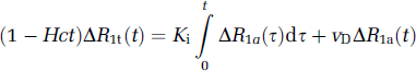
Consider the middle of our three nested models, the original Patlak model (Model 2) (Table 1). It is a model of the blood-brain exchange of an indicator (Patlak and Blasberg, 1985; Patlak et al, 1983) that has one very critical, simplifying assumption. This assumption is that there exists an ‘irreversible’ tissue region beyond the BBB, where the tracer is essentially trapped for the duration of the experiment. The working equation for this system is:

C_{t} (t) = K_{i} \int_{0}^{t} C_{p} (τ) d τ + v_{d} C_{p} (t) + v_{a} C_{p} (t)

(1)

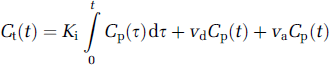
where C_p and C_t are the plasma and tissue concentrations of the indicator, K_i is the unidirectional transfer constant of the indicator from plasma across the barrier into the interstitial fluid, v_d is the fractional volume of the rapidly reversible, plasmatracking tissue space, and v_a is the fractional volume of the plasma (Table 2 lists definitions and symbols). Since they cannot be estimated separately from the data, v_d and v_a will hereafter be combined into one volume fraction, v_D.

Table 1

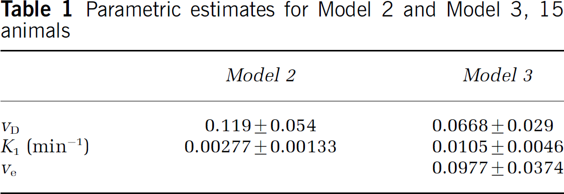
Parametric estimates for Model 2 and Model 3, 15 animals

	Model 2	Model 3
V_D	0.119 ± 0.054	0.0668 ± 0.029
K₁ (min⁻¹)	0.00277 ± 0.00133	0.0105 ± 0.0046
V _e		0.0977 ± 0.0374

Table 2

Symbols, with units of measure

Symbol	Use (units)
C_p(t)	Plasma concentration as a function of time (mL tracer/mL plasma)
C _R	Relaxivity of the contrast agent in units of (ms⁻¹ per unit concentration)
C_t(t)	Tissue concentration as a function of time (mL tracer/mL tissue)
Hct	Hematocrit as a fraction of blood volume (mL erythrocytes/mL blood)
k _b	Transvascular unidirectional (inward) transfer constant (min⁻¹)
K _i	Transvascular unidirectional (outward) transfer constant (min⁻¹)
R _1a, R _1P	Arterial, erythrocyte, and plasma (respectively) longitudinal relaxation rates (ms⁻¹)
ΔR_1a, ΔR_1t	The change, due to the injection of contrast agent, in the arterial (subscript a) and tissue (subscript t) longitudinal relaxation rates (ms⁻¹)
R_1tiss, R₁	Tissue, cellular, and extravascular extracellular (respectively) longitudinal relaxation rates (ms⁻¹)
S _e, S _p, S _f	Summed-squared residuals between the model and the data: extra, partial, and full, respectively
t	Time (min)
τ(Greek tau)	Dummy variable of integration of time-varying quantities
v _d	Fractional volume of rapidly equilibrating reversible space (mL/mL tissue)
v _a	Fractional volume of plasma (mL/mL tissue)
V_D = V_d+V_a	Combined fractional volume of plasma and rapidly equilibrating non-plasma spaces (mL/mL tissue)
v _e	Extravascular, extracellular volume fraction (mL EES/mL tissue)
v'_d	The y-axis intercept of the linear portion of the Patlak plot in the event that an initial portion of the arterial input function is not measured
v_e,v_p,v_f, (Greek nu)	Degrees of freedom for extra, partial, and full summed-squares
(1 - Hct)ΔR_1tiss(t)/ΔR_1a(t)	Patlak plot ordinate
$\frac{\int_{0}^{t} Δ R_{1 a} (τ) d τ}{Δ R_{1 a} (t)}$	Patlak plot abscissa
$\int_{0}^{t} Δ R_{1 a} e^{- k_{b} (t - τ)} (τ) d τ$	Efflux-corrected Patlak plot abscissa

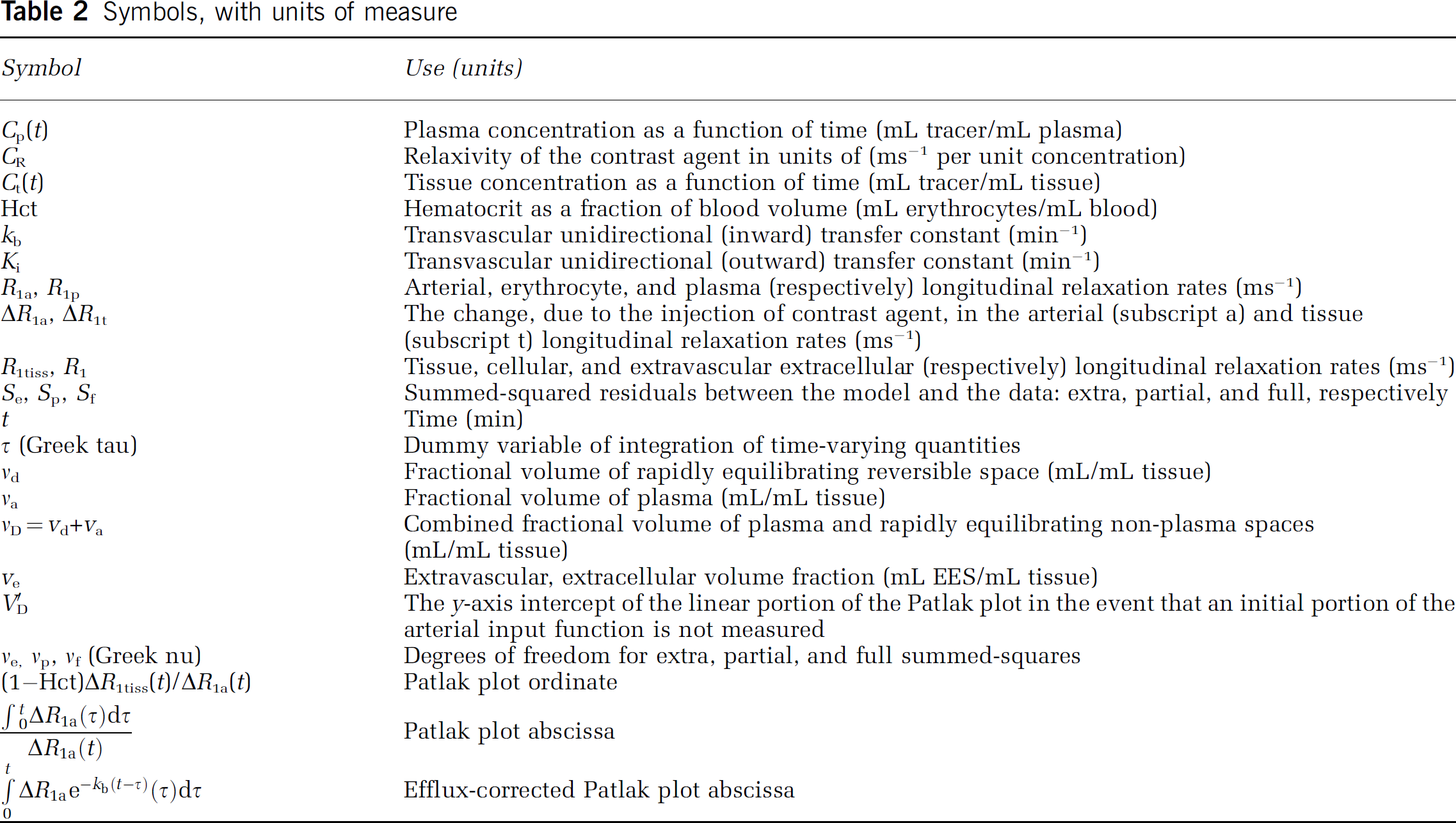
In this and all following expressions, units will follow ‘MRI conventions,’ in which concentrations are in mL indicator/mL tissue, flows and permeability-surface (PS) products are in min⁻¹, etc. This is in distinction to the ‘radiological conventions,’ in which concentrations are in mL indicator/g tissue), and PS products are in mL/gmin. Numerically, since the density of brain tissue is very close to 1, the two unit systems produce estimates of transfer constant and distribution volume that are nearly identical.

Patlak et al have introduced a method for linearizing the problem of curve fitting. A graph of the ratio C_t(t)/C_p(t) versus $\int_{0}^{t} C_{p} (τ) d τ / C_{p} (t)$ (generally this abscissa is called ‘stretch time’) yields a linear relationship, with a slope of K_i and an ordinate intercept of v_D. Such a graph has become known as the Patlak plot (Gjedde, 1997; Patlak et al, 1983). For our purposes, this linearization is useful because it makes model testing via F-test comparisons exact (see below).

In a later modification (Patlak and Blasberg, 1985), a correction for efflux from the ‘irreversible’ tissue compartment back into blood was obtained:

C_{t} (t) = K_{i} \int_{0}^{t} e^{- k_{b} (t - τ)} C_{p} (τ) d τ + v_{D} C_{p} (t)

(2)

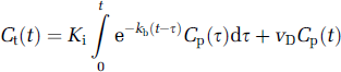
where the additional term, k_b, is the transfer rate from the extravascular ‘irreversible’ compartment to the plasma compartment and removal by the circulation. This equation is exactly equivalent to that of the ‘consensus’ model (Tofts et al, 1999). The equivalence between the consensus model notation and the variables above are as follows: K_i = K^trans, K = K_ep, v_D = V_b (this latter equivalence is approximate, since v_D as defined differs slightly from the blood volume itself). Hereafter, the notation of Patlak will be followed because it: (1) takes precedence over the later consensus model; (2) is unified among the three models examined; and (3) is closer to standard scientific usage since, in the main, it uses single-character subscripted variables to represent physical variables.

In terms of model testing, introducing k_b extends Model 2 by testing its central assumption of no backflux across the BBB. As in the original Patlak treatment, if the quantity C_t(t)/C_p(t) is plotted versus the efflux-corrected arterial time integral $\int_{0}^{t} e^{k_{b} (t - τ)} C_{p} (τ) d τ$ divided by C_p(t), a linear plot should result, with a slope of k_b and an intercept of v_D. The term k_b corresponds to K_i/v_e where v_e is the extravascular, extracellular space.

The Observation Equations

As detailed elsewhere (Cao et al, 2005), we assume the fast exchange limit for the protons of water in both tissue and blood. In this case, the observation equation equivalent to equation (1) is

(1 - H c t) Δ R_{1 t} (t) = K_{i} \int_{0}^{t} Δ R_{1 a} (τ) d τ + v_{D} Δ R_{1 a} (t)

(3)

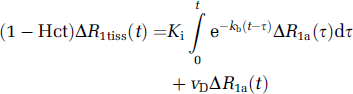
where Hct is the hematocrit, R_1a is the longitudinal relaxation rate of all protons in the artery, R_1t is the longitudinal relaxation rate of all protons in the tissue, and Δ refers to the subtraction of the precontrast rate from its postcontrast value. Plotting the ratio (l-Hci)ΔR_1t(t)/ΔR_1a(t) versus $(\int_{0}^{t} Δ R_{1 a} (τ) d τ) / (Δ R_{1 a})$ yields the Patlak plot (Model 2), with a slope of K_i and an ordinate intercept of v_D. If K_i is approximately zero, the model (Model 1) will incorporate only the distribution volume, v_D.

The observation equation that corresponds to equation (2) (Model 3) and corrects for efflux from the ‘irreversible’ compartment is

\begin{matrix} (1 - H c t) Δ R_{1 t i s s} (t) = & K_{i} \int_{0}^{t} e^{- k_{b} (t - τ)} Δ R_{1 a} (τ) d τ \\ + v_{D} Δ R_{1 a} (t) \end{matrix}

(4)

We will show an example of both the original Patlak plot and the efflux-corrected version, show in a sample of 15 animals the changes in the parametric estimates v_D and K_i that result from this correction, and offer a criterion for choosing between the various models, that is, between no appreciable leakage of MRCA across the BBB, leakage of MRCA with negligible tissue efflux, and leakage with appreciable tissue efflux.

The Effect of Missing Initial Arterial Data

Let us assume that, for some initial period t≤t₀, neither tissue nor arterial data are determined, and the measurement is taken up after t₀. As detailed in the appendix, the apparent distribution volume, V'_D, should be related to the true distribution volume via the following:

V_{D}^{'} = \frac{K_{i} \int_{0}^{t_{0}} C_{p} (τ) d τ}{C_{p} (t_{0})} + v_{D}

(5)

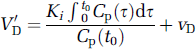
and a plot of V'_D versus K_i with group data will display a relationship with a slope equal to $(\int_{0}^{t_{0}} C_{p} (τ) d τ) / (C_{p} (t_{0}))$ and a y-intercept equal to the actual distribution volume, v_D.

Materials and methods

Animal Preparation—9L Tumors in Fischer 344 Rats

Fifteen male Fischer 344 rats (weight 220 to 300g) were studied in a protocol approved by the Henry Ford Health Systems animal care committee.

The 9L tumor is a well-characterized rat brain tumor model (Moulder and Rockwell, 1984; Wheeler and Wallen, 1980). Obtained from Dr Kenneth Wheeler, Wake Forest University, the tumor line was originally derived from rat brain after induction by intravenous N-nitrosomethylurea. Cells were maintained by serial passage in vitro using Dulbecco's medium and 10% fetal bovine serum. The rat's head was immobilized using a small animal stereotactic device (Model 902, Kopf Instruments, Tujunga, CA, USA). After a midline incision, the skull was exposed and a burr hole drilled through the skull, taking care not to penetrate the dura. In all, 10,000 9L rat cells were injected at a rate of 1 μ/L/min into a location 2.5 mm anterior to the bregma, 2.0 mm to the right of the midline, and a depth of 3.0 mm, as described previously (Kim et al, 1995). After implantation, the animals were returned to their cages for a period of approximately 16 days. Untreated 9L brain tumors are typically 2 to 3 mm in diameter on days 14, and 5 to 6 mm in diameter on day 18 (Brown et al, 1999).

Magnetic resonance imaging was performed 16 ± 2 days after cell implantation. Each rat was anesthetized with 3.0% halothane for induction, and then spontaneously respired with 1.0% to 2.0% halothane in a 2:1 N₂O:O₂ mixture using a face mask. Body temperature was maintained constant (37°C) with a recirculating water pad monitored via an intrarectal type T thermocouple. Femoral arterial and venous PE-50 catheters were inserted to obtain blood samples, record systemic arterial pressure, and inject the MRCA.

Magnetic Resonance Imaging

Magnetic resonance imaging procedures employed a 7T, 12 cm (clear bore) Magnex magnet with actively shielded gradients of 250mT/m and 100 μs rise times. The magnet was interfaced with a Bruker Avance console running Para vision V2.1.1. The RF coils were a Bruker volume resonator for transmission and an actively decoupled 2 cm Bruker surface coil for reception. The volume resonator, animal holder, and surface coil formed an imaging unit to be inserted in the magnet. After animal location in the holder, the surface coil was centered over the brain, the holder was located in the volume coil, and the imaging apparatus and animal were located in the magnet. Using a three-plane sequence, the central imaging slice was placed to view the largest lateral extent of the tumor.

Since the change in the longitudinal relaxation rate, R₁(R₁ = 1/T1) is generally thought to be linear in concentration of MRCA, this measurement is critical in estimating vascular permeability. A T-One by Multiple Read-Out Pulses (TOMROP) (Brix et al, 1990) sequence, developed on a 3T human system (Gelman et al, 2000), was adapted to the requirements of the 7T animal system (Ewing et al, 2003a).

T-One by Multiple Read-Out Pulses is a Look-Locker sequence (Look and Locker, 1970), and thus an efficient and unbiased estimate of T₁ (Crawley and Henkelman, 1988). At least one dummy cycle N pulses followed by T_relax) was applied before the start of data acquisition. Inversion of the longitudinal magnetization was accomplished using a nonselective hyperbolic secant adiabatic pulse of duration 12 ms. One phase-encode line of 24 small-tip-angle (approximately 18° shaped pulses) gradientecho images (echo time, TE 4 ms) was acquired after each such adiabatic inversion, at 50-ms intervals, for a total recovery time of 1200 ms with a 2-sec relaxation interval between each adiabatic inversion. Matrix size was 128 × 64, field-of-view (FOV) 32 mm, three 2-mm slices.

All images were obtained with 32 mm FOV. Before the administration of MRCA, a single-slice arterial spin labeling (ASL) perfusion study (Ewing et al, 2003b) (matrix 64 × 64), a high-resolution T2-weighted image set (repetition time (TR)/TE = 2000/10 ms, 3 CPMG echoes, matrix 256 × 192 seventeen 0.5-mm slices, 4 accumulations), a T1-weighted high-resolution image set (TR/ TE = 1000/7.5, matrix 256/192, 27 0.5 mm slices, 4 accumulations), and two baseline TOMROP studies were obtained. Magnetic resonance contrast agent (250/μmol/kg) was administered in a 0.2 mL bolus over approximately 4 sees. The dynamic contrast created by the bolus was followed with an echo-planar spin-echo sequence (TR/ TE = 1000/32, matrix 64 × 64, three 2 mm slices) for a total of 64 scans, with bolus administration beginning on the tenth scan. Immediately after the echo-planar sequence, 10 TOMROP sequences were run, following the tissue concentration of MRCA across a 25-min period. After the last TOMROP study, a postcontrast Tl-weighted image, identical to the precontrast study, was acquired. Data from the Echo-Planar study will be reported separately. We note, however, that approximately 1 min separated the administration of the contrast agent and the beginning of the first postcontrast TOMROP acquisition.

Using the postcontrast T1-weighted image, each slice was examined for the presence of tumor; if leakage was seen, the area of leakage was outlined manually, filled, and the volume of tumor in the slice calculated by multiplying the area of leakage by the slice thickness. All such volumes were summed, thus yielding an estimate of total tumor volume.

Data Analysis

Using TOMROP image sets taken at 145-sec intervals, pixel-by-pixel R₁ maps were constructed using a maximumlikelihood procedure constrained to yield nonnegative estimates of the model parameters (Gelman et al, 2000).

Three 2-mm-thick slices of data on 2 mm centers were available. The slice with the largest extent of tumor was selected for further study. In most, but not all, cases, this was the center slice of the three-slice package. Sagittal ΔR₁ was measured in the slice where that sinus was most easily visualized and used to estimate the ΔR₁ of cerebral arterial blood, a practice previously validated (Ewing et al, 2003a).

As we have noted, the tissue ΔR₁ was used as a measure of tissue MRCA concentration. Equations (3) and (4) were used to produce pixel-by-pixel estimates of K_i and v_D, assuming arterial hematocrit to be 0.45. To visually evaluate the linearity of the data in tissue with abnormal BBB permeability, a region of interest (ROI) was selected and demarcated in each animal by examination of the postcontrast T_1-weighted image. Using sagittal sinus data and ROI ΔR₁'s, Patlak plots (Models 1 and 2) and efflux-corrected Patlak plots (Model 3) were constructed for each pixel within the ROI. In those cases where the single-slice ASL technique and the slice with the largest extent of tumor coincided, CBF was measured pixel-by-pixel across the brain.

The general characteristics of the transfer constants by the three models are: Model 1, K_i = 0, k_b = 0; Model 2, K_i>0, k_b = 0; and Model 3, K_i>0, k_b>0. The summed-squared residuals of the data plotted according to the three models was computed pixel by pixel, and the F-statistic calculated (Bates and Watts, 1988). The results were then compared 1 versus 2, and 2 versus 3; that is, first a model with no leakage was compared with one with irreversible leakage and then a model with irreversible leakage was compared with one with reversible leakage. The F-statistic was computed and mapped on a pixel-by-pixel basis and also computed for the entire ROI. The ROI uncorrected and efflux-corrected Patlak plots were also examined visually. Because of the continuous decrease in blood concentration of MRCA, the later time data were less reliable than those from earlier times. For this reason, we systematically reduced the data set, point-by-point, until the 2 versus 3 F-test reached a maximum. For instance, we might have started with 11 data points, but found that the Model 2 versus 3 F-test peaked at 9 points. In this case, the parametric estimates from both models for 9 fitted points were used in reporting the data. In all cases, at least six points were used.

Statistical Tests—Model Comparisons

An ‘extra sum of squares analysis for nested variables’ (Bates and Watts, 1988) was employed to examine which model best resolved the data. In the following, the Patlak model will be referred to as the partial model, and the efflux-corrected model as the full model. The ratio (S_e)/v_e)/ (S_f/v_f was computed, where S_e and S_f are sum-squared residuals (further described below), the subscript e refers to the full model, and the subscript e refers to the extra variance accounted for by the full model relative to the partial model. The degrees of freedom v_e and v_f are, in this case, 1 (for the number of extra parameters in the full model), and N—m, where N is the number of points on the clearance curve, and m is the number of parameters in the partial model (m = 2 for Model 2, m = 3 for Model 3). It is further defined that S_e = S_p—S_f where S_p is the sum of the squared residuals of the partial model, and S_f is the sum of the squared residuals of the full model. For linear models, the ratio (S_e/v_e)/(S_f/v_f) is distributed as the F-statistic, F_{Ve, VF}, with v_e and v_f degrees of freedom.

In the F-test, the null hypothesis is that the two samples of sum-squared residuals were drawn from the same pool, that is, the two models are equivalent. The failure of this hypothesis leads to acceptance of the larger model (the model with the smaller sum-squared residuals). The probability associated with the F-test (the P-value) is that of a Type I error, for example, the probability of accepting Model 3 when the underlying truth was that of Model 2. In the problem at hand, we placed the threshold for acceptance of the larger model at P = 0.05, Bonferonni-corrected for (two) multiple comparisons. The F-test threshold for each of the model comparisons was, thus, set at P<0.025.

As for reporting other data and comparisons, mean±standard deviation is given, and standard statistical tests are indicated where employed.

Results

Fifteen animals were studied. Mean tumor age was 15.9±2.1 days (range 14 to 22 days). As measured by the postcontrast Tl-weighted images, mean tumor volume, which varies exponentially with time after implantation, was 70.0±64 mm³ (range 5 to 229 mm³). For the nine animals in which the slice of the CBF study coincided with the tumor slice, mean flow was estimated at 2.0±0.9 min⁻¹.

To introduce the findings, the data from a single animal studied 16 days postimplantation will be presented. In this case, total tumor volume was 121 mm³. Images of the (0.5-mm thick) center slice of the post-Gadomer T1-weighted image (taken approximately 25 mins after injection) and a (2-mm thick) map of CBF are shown in Figure 1. These images show the heterogeneity of microvascular leakage and CBF, respectively, typical of 9L tumors. This tumor had a mean flow rate (assuming the tissue density to be approximately 1.0) of 1.41 min⁻¹.

Figure 1

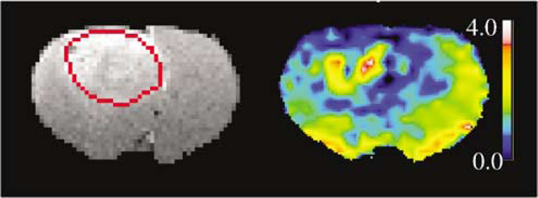
Left: Postcontrast T₁-weighted image, resolution reduced to 128 × 128, with region-of-interest outlined in red. Right: Pseudocolor map of CBF; (mL/lOOg min) produced by a single-slice ASL technique. The color bar demarcates a set of ranges of CBF with blue the lowest and pink the highest. A ‘bulls-eye’ pattern of flow, with notable heterogeneity, is visible in and around the tumor region.

The time course of ΔR₁ in the sagittal sinus blood (Figure 2, scaled by a factor of 4) and the tumor ROI (Figure 2) were typical of a bolus injection. Since the constant of proportionality is the same for blood and tissue, ΔR₁ indicates MRCA concentration in both over the duration of the experiment. From these data, a Patlak plot according to equation (3) and efflux-corrected Patlak plot (equation (4)) were made (Figure 3). For the former (Model 2), v_D and K_i were estimated to be 0.170 and 0.00312 min⁻¹, respectively, whereas, for the efflux-corrected plot (Model 3), they were determined to be 0.0835 and 0.0116 min⁻¹, respectively. Additionally, k_b was estimated to be 0.0798, which yields a V_EES of 0.145. The discrepancy in the output between Model 2 and Model 3 is almost certainly related to the curvature of the Model 2-derived Patlak plot beyond the first three points (i.e., after 9 mins real time, the period of negligible Gadomer efflux in this instance). A visual examination of these two plots across the entire duration of the experiment indicates the superiority (better linearity) of the efflux-corrected plot.

Figure 2

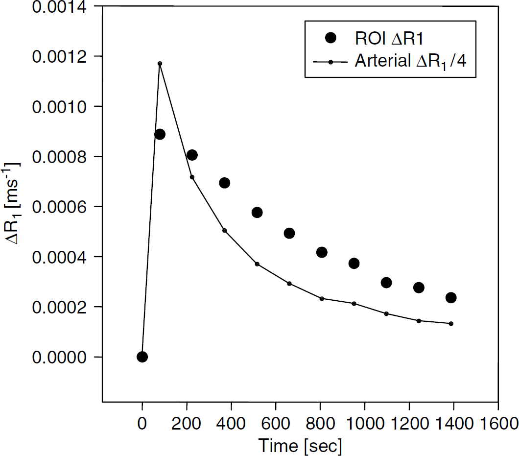
Sagittal sinus ΔR₁ (divided by 4.0) and ROI ΔR₁ in rat je29 versus real time. The time record of sagittal sinus ΔR₁ (adjusted for hematocrit) was taken to be proportional to the arterial concentration of contrast agent concentration, and the ROI ΔR₁ was proportional to tumor contrast agent concentration.

Figure 3

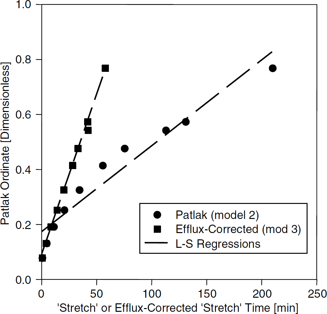
Blood and tissue concentration data from rat je29 plotted against respective ‘stretch’ times for the two models (real time = 25 min). Circles: plotted via Patlak graphical method (Model 2) for estimating K_i-. Squares: plotted via Patlak graphical method with correction for tissue efflux (Model 3). Regression lines show least-squares best fits for both models. The slope of each regression line yields an estimate of the transfer constant associated with its model.

The more formal and objective F-test analysis confirms this impression. As indicated in Materials and methods, two comparisons of F-test outcomes were made among the models: Model 1 versus Model 2 and Model 2 versus Model 3. With 10 points to fit, the degrees of freedom for the first test were 1 and 8, and for the second 1 and 7. The F-tests yielded 129 for the first comparison and 164 for the second (P<0.001 for both tests), thus rejecting Model 1 (no leakage of Gadomer) in favor of Model 2 (irreversible leakage) and Model 2 in favor of Model 3 (reversible leakage).

The pixel-by-pixel maps of v_D and K_i from Model 2 and Model 3, as well as a map of the F-statistic and k_b, show considerable heterogeneity within the tumor of this rat (Figure 4). The parameter k_b (Figure 4F) should be masked by a map of the F-statistic (Figure 4E); when the F-statistic is not large, k_b might not have a meaningful value because the model which generates this parameter is not supported by the data. Not shown but also produced were maps of Model 1 estimates of v_D, and the F-statistic comparing Model 1 with Model 2. As already noted, the regional tumor values of v_D and K_i differ between Models 2 and 3; the two methods also produce maps which differ in pattern within the tumor. While this impression has not been formally tested, the Model 2 map of v_D (Figure 4A) resembles the Model 3 map of K_i (Figure 4D). We suggest that the curvature of the uncorrected Patlak plot produced by appreciable MRCA efflux from the tissue moves the y-intercept of the linear plot upward (compare the intercepts of Models 2 and 3 in Figure 3).

Figure 4

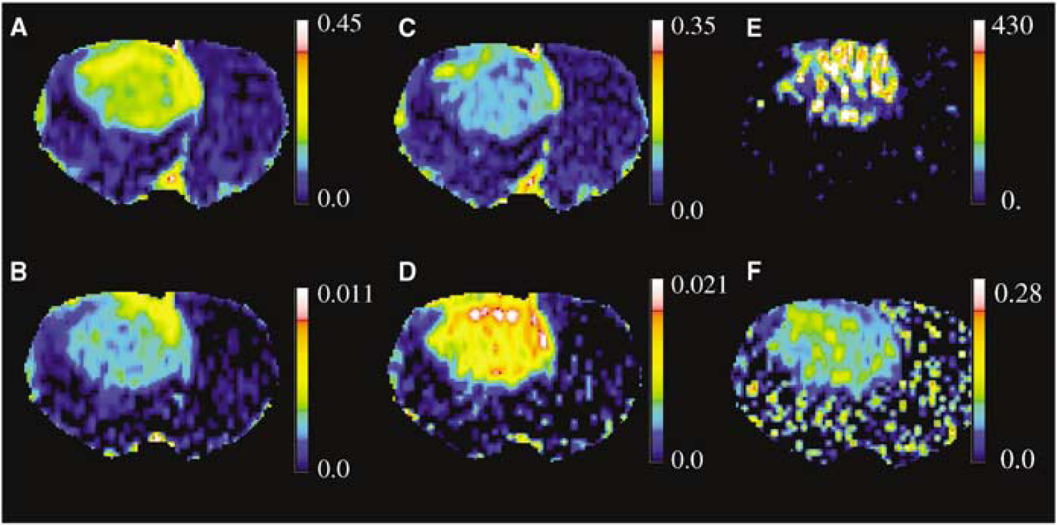
Pixel-by-pixel pseudocolor, parameter maps in the animal used as an example in the text and Figures 2 and 3. (A) Model 2 estimate of v_D; (B) Model 2 estimate of K_i (min⁻¹); (C) Model 3 estimate of v_D; (D) Model 3 estimate of K_i (min⁻¹); (E) F-test for Model 2 versus Model 3; (F) tissue-to-vascular efflux constant, k_b (only valid for regions where F-test is significantly large). The color bars demarcate sets of ranges of each parameter.

Finally, the estimate of v_D produced by Model 1 was masked to select areas in which there was no advantage of Model 2 over Model 1, which is to say that these were areas within the ROI with little or no Gadomer leakage and relatively normal microvessels. The mean value of v_D in these areas with normal BBB function was 0.0312. Assuming hematocrit of 0.45, this yields a plasma volume of 0.014, which is approximately consistent with previously performed estimates of cerebral plasma volume using radiotracers (Bereczki et al, 1992).

As for the group data, the F-test comparing Model 2 to Model 1 exceeded 10 (P< 0.025) in all animals, and Model 3 was always superior to Model 2 for the tumor ROI across the 15 animals. In accordance with this, the mean v_D of Gadomer in the group was found to be approximately twofold larger with Model 2 than Model 3, whereas the mean K_i of MRCA with Model 2 was approximately 30% of that with Model 3 (Table 1). As expected, the application of the original Patlak model to data from these experiments yields an overestimation of v_D and an underestimation of K_i. The Model 3 values for v_D (approximately 7%, Table 1), transfer constant, and extravascular, extracellular space (around 10%) characterize this tumor as vascular with a moderately leaky BBB (mean plasma flow approximately 11-fold greater than mean influx rate) and a fairly normal extra cellular space. The latter space indicates that the tumor is mainly made up of viable, Gadomer-excluding cells and is not necrotic. As shown below, the microvascularity of the tumor might, however, be overestimated because v_D was probably biased high, the result of missing the initial part of the arterial input function.

While the two models produce different transfer constants, the estimates are not unrelated. When the K_i's produced by Models 2 and 3 are graphed against each other for the individual experiments (Figure 5) and tested, the two estimates are highly correlated (r = 0.80, P = 0.0003). The intercept of the regression line, 0.0029 ± 0.0017 (min⁻¹), is not significantly different from zero (P>0.1), implying that there is a convergence of the influx rate estimates of the two models as K_i decreases. We reason that, since the concentration of MRCA in the interstitium is low when influx is low, tissue-to-blood efflux is minimal, and the linearity of Model 2 will be indistinguishable from that of Model 3.

Figure 5

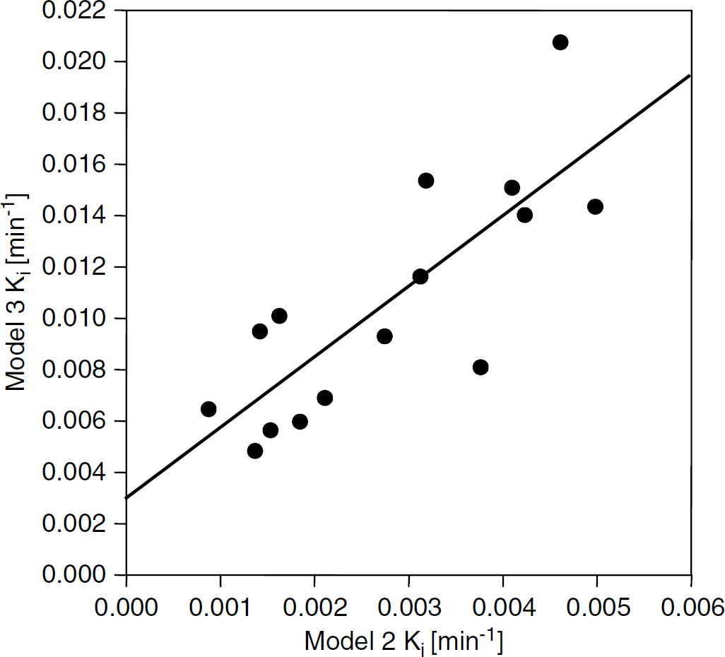
Model 2 estimates of K_i versus Model 3 estimates in ROIs selected to be within the tumor boundaries. Correlation coefficient between the K_i values, r = 0.80 (P<0.0003). Zero intercepts = 0.0029±0.0017, not significantly different from 0 (P>0.1). The two estimates in this model system, while different in magnitude, are highly correlated.

As for the bias introduced into the estimate of v_D by missing arterial data, Figure 6 is a plot of V_D' versus K_i. If the relationship of equation (A3) holds (see appendix), then the slope of this line should estimate the quantity $\int_{0}^{t_{0}} C_{p} (τ) d τ / C_{p} (t_{0})$ and the intercept should approximate the true distribution volume v_D. In this case and for the group of animals studied, the y-intercept is 0.016 ± 0.013, which is probably closer to the real mean distribution volume of the indicator within the microvascular system of the rat 9L tumor at 16 days after implantation. The slope of the regression plot is 4.9 ± 1.1, meaning that the ratio of the integrated input function to the first point plasma estimate of the Gadomer concentration-time product is approximately 5:1. Although the estimate of v_D is biased high by missing the initial part of the arterial input function, it is notable that, since the plot of Figure 6 uses the full estimate of K_i to produce this reasonable group estimate for v_D, we can infer that K_i is relatively insensitive to this experimental shortcoming.

Figure 6

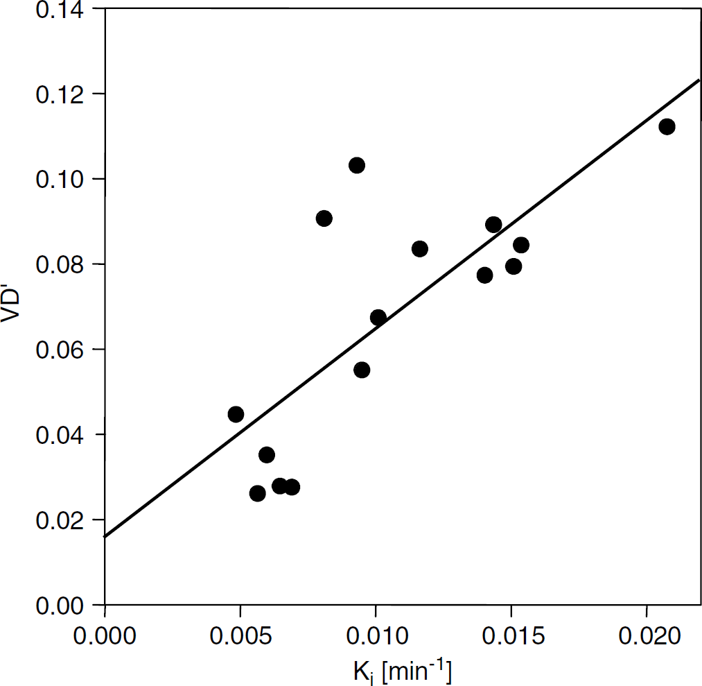
V'^D versus K_i in the various ROIs of the 15 animals. The group estimate of v_D is 0.016 ± 0.013. For this group of animals, with gadomer administered in a bolus, the estimate of the quantity $\int_{0}^{t_{0}} C_{p} (τ) d τ / C_{p} (t_{0})$ equals 4.9 ± 1.1 min.

Discussion

Fifteen rats implanted with an aggressive cerebral 9L tumor were studied using MRI and a large (17kDa), Gd-tagged MRCA. The aim of the study was to establish the operating characteristics of MRI estimates of the blood-to-tumor transfer constant.

Gadomer is a dendritic Gd chelate containing 24 Gd nuclei per molecule, with a real molecular weight of approximately 17 kDa, but an effective one of approximately 33 kDa. Because of its effective size, it should approximate radioiodinated serum albumin (RISA) when used as a measure of vascular permeability. In an examination of changes in RISA distribution in the RG-2 glioma model induced by administration of dexamethasone, Nakagawa et al (1987) determined a mean K_i of 0.0236 ± 0.0089 μ/g min in untreated rats, approximately twice the value we report for Gadomer in 9L tumors. The extravascular volume in the RG-2 tumor was 0.137 ± 0.016 mL/g, in approximate agreement with our 9L estimate, and the plasma volume was estimated to be 0.0155 ± 0.013 mL/g (Nakagawa et al, 1987). Using a large-vessel hematocrit of 0.45, our corrected estimate for vascular volume of approximately 0.016 ± 0.013 ml/ml yields a small-vessel plasma volume of approximately 0.0072 ± 0.0059, which is smaller than, but not significantly different from, that of Nakagawa et al. The RG-2 glioma used by Nakagawa is an aggressive, infiltrating, and nonimmunogenic tumor that is typically wellperfused. Except for its lack of immunogenicity, it closely resembles the 9L tumor model in growth rates and survival times.

Other MRI experiments with tumor models have estimated transfer constants for Gadomer. In spontaneous canine mammary tumors, Henderson et al (2000) measured K_i of 0.014 ± 0.011 min⁻¹ for Gadomer, which is virtually identical to the figure for the 9L cerebral tumor (Table 1). Ivanusa et al (2001), working with a mouse fibrosarcoma SA-1 tumor, estimated the PS area product of Gadomer to be 0.0113 ± 0.005 min⁻¹. The influx transfer constant is, by definition, related to the extraction fraction via the following: K_i = FE = F(1-e-^−(PS/FV)), where F is the blood flow and V is the volume fraction of the plasma. If, as in our leaky tumors, PS/FV≤1, then a Taylor expansion shows that Ki ≈ PS and our K_i values approximate PS. Thus, Ivanusa's estimate is again virtually identical to our estimate for the 9L cerebral tumor. In contrast, Verhoye et al (2002), using human xenograft tumors intracerebrally implanted in rats, found Gadomer transfer constants that were roughly 10 times larger than those we estimated for the rat 9L cerebral tumor. As a possible explanation of this discrepancy, implanted xenografts tend to be invaded by new blood vessels that are rather leaky, whereas 9L tumor cells infiltrate the surrounding tissue with its already existing microvascular system and its initially impermeable capillaries.

In a prior MRI study of a rat transient ischemia model with Gd-DTPA, the K_i values obtained with simple Patlak plots (Patlak et al, 1983) were highly correlated with autoradiographic (ARG) single-time point estimates of K_i for ¹⁴C-sucrose, a molecule similar in size to Gd-DTPA (Ewing et al, 2003a). A preliminary study on this same ischemia model with Gd-DTPA as the MR contrast agent and relabeled Gd-DTPA as the ARG tracer corroborate the preceding finding, showing good agreement between the Gd-DTPA influx constants determined by the two different techniques.

In their original publication, Patlak et al clearly stated that the purpose of the multiple-time graph was to check the plotted data for linearity. If linearity was found for all or part of the curve, then influx dominated the distribution process during that period, and the slope of the line was equal to the influx constant. If not found, then this approach cannot be used. Such testing was performed (Ewing et al, 2003a), with no strong evidence of nonlinearity observed; K_i was subsequently evaluated from the line.

In the present tumor study, nonlinearity was apparent across the typical time period of an experiment, even when Gadomer—a much larger and presumably less permeable MRCA than Gd-DTPA—was employed. Accordingly, the generalized Patlak graphical approach (Patlak and Blasberg, 1985) was applied. If the variable k_b in equations (2) and (4) is understood to equal K_i,v_e then the generalized Patlak approach and the consensus model are formally identical. This provides a valuable linkage between the Patlak graphical approach for MRI data and the consensus approach. In fact, the generalized Patlak, the original Patlak, and the hypothesis of no leakage at all form a set of nested models, which we have labeled 3, 2, and 1, respectively, to indicate the number of parameters estimated in each. These series of models collectively form an extended methodology for MRI studies of vascular permeability.

That the underlying models examine the linearity of the blood and tissue data is important, since it considerably simplifies the job of comparison between them, both in statistical theory and in the very necessary visual inspection of the plots. An examination of Figure 3, for instance, reveals that the data graphed under Model 2 are clearly nonlinear after the first 3 points, whereas those plotted under Model 3 form a straight line over the entire period of the experiment. To look at this in a different way, however, the first three points of Figure 3 plotted via Model 2 form a decent straight line and define a short period of linearity, are virtually identical to those of Model 3, and yield similar values of K_i and v_D.

Model 3 offers the best resolution of our data and the best estimates of v_D and K_i- In setting a threshold for the acceptance of an F-test, it was judged that a Type I error (i.e., accepting evidence for nonlinearity when there was none) would not be a damaging error. In the worst case, some additional error might be introduced to the estimates of v_D and K_i-. This outcome was judged to be nonthreatening, and the level of acceptance of this type of error set to 5%, Bonferroni-corrected for multiple comparisons. Our experience with this criterion has generally been positive, with the outcomes matching visual examination.

In our previous study of a transient ischemia model (Ewing et al, 2003a), the agreement of Model 2 estimates of K_i with those of autoradiography did raise the question as to why MRI estimates of v_D were much higher than might be reasonably expected for the blood volume of a ischemia-injured tissue, and in fact higher than an estimate produced by dynamic contrast studies conducted immediately before the permeability studies. One possibility— that enhanced water exchange across a damaged BBB increased the effect of the MRCA—has been ruled out on theoretical grounds (Cao et al, 2005). Two other possibilities, which are not mutually exclusive, remain.

First, the artifact could be attributed to a significant nonlinearity in the Patlak plot introduced by tissue-to-vascular efflux. The efflux-corrected Model 3 estimates of v_D were approximately half those found with uncorrected Model 2. The second likely source of artifact was our decision to use a different MRI sequence to follow the initial period of indicator circulation and uptake, the missing data problem. Our subsequent analysis indicated that the missing blood data could be found in the y-intercept of the Patlak plot and that the estimate of v_D from the plot should vary linearly with K_i- With the assumption that the arterial concentration-time course varied little from animal to animal, the amount of missing blood data and a better estimate of v_D could be evaluated from the tissue-blood findings of the entire group of rats. In this case, this contribution reduced the estimate of v_D from 6.7% to 1.6%.

Some consideration of our experimental design is in order. The sampling rate was approximately 145 sees per point for the 25-min period. It was slower than other recent experiments and is not practical if these procedures are to be translated to human brain tumor studies. Moreover, we note from inspection that the first three points—approximately 9 mins (Figure 3)—of most Patlak plots were coincident for Models 2 and 3, thus defining an interval in which it can be expected that MRCA efflux is negligible and Model 2 estimates of transfer constant can be used. In situations where influx is comparable to that of the current work and MRI data can be obtained at 1-min intervals, then the first 5 to 10 min of data might be linear by Model 2 analysis, and the transfer numbers might be measurable without further modification. This is important to recognize when, for example, to compare multiple-time MRI estimates of microvascular permeability in brain tumor models with those of single-time ARG measurements.

Sampling ‘as fast as possible’ might not be ideal, since this complicates the task of estimating the arterial input function, and raises the problem of timing the arrival of indicator in the tissue. We chose to sample slowly enough so that the change in sagittal sinus indicator concentration could be taken as the arterial input function. The validity of this approach depends on several assumptions. First, most of the tissue draining into the saggital sinus is assumed to be normal and no MRCA is lost from the blood into brain en passage through such portions of the brain. Second, it is presupposed that the presence of the tumor itself does not extract sufficient MRCA from the blood to seriously affect the shape of the venous concentration curve. Thirdly, the lag time between MRCA passage through the microvascular networks and sagittal sinus (3 to 6 sees) is assumed to not introduce a significant uncertainty into the timing of the experiment.

The second assumption is particularly important, since it interacts with the first-pass extraction of the MRCA. If there is a large first-pass extraction, it is necessary to sample the tissue curve at high frequency and determine the input function in an artery close to the tissue. This points to the difficulties presented in the current clinical setting, where only small MRCAs (less than lkDa) are approved for use in humans. In aggressive tumors, or any other lesion with highly permeable microvessels, quantifying vascular permeability via MRCA uptake and clearance may become extremely difficult because of the necessity for rapid and precise estimates of MRCA concentration in both arterial blood and tissue. This suggests the need for clinically approved macromolecular MR contrast agents.

While the experimental design of permeability studies in an aggressive cerebral tumor has been investigated herein, the need for protocol flexibility in other settings must be emphasized. Among the various neuropathological models, there is almost certainly a broad range of microvascular permeabilities between and within lesions. This necessitates the selection and usage of an MRCA of appropriate size, a duration of study, and analytical models that fit the operating characteristics of the permeability measurement. To its advantage, the expanded or serial Patlak graphical approach offered in the present work linearizes an essentially nonlinear problem, allows the visual examination of data for the period of linearity, formally tests for alternative models, and even evaluates the systematic errors due to missing arterial data.

Footnotes

Acknowledgements

The authors wish to thank Schering AG for its gift of Gadomer for use in the sample of animals of this paper. We owe a great debt to Clifford Patlak for the many illuminating phone conversations we had with him concerning the analyses herein.

Appendix

References

Bates

Watts

(1988 Nonlinear regression analysis and its application. New York: John Wiley and Sons

Bereczki

Wei

Acuff

Gruber

Tajima

Patlak

Fenstermacher

(1992) Technique-dependent variations in cerebral microvessel blood volumes and hematocrits in the rat. J Appl Physiol 73:918–24

Bhujwalla

Artemov

Natarajan

Solaiappan

Kollars

Kristjansen

PEG

(2003) Reduction of vascular and permeable regions in solid tumors detected by macromolecular contrast magnetic resonance imaging after treatment with antiangiogenic agent TNP-470. Clin Cancer Res 9:355–62

Brix

Schad

Deimling

Lorenz

(1990) Fast and precise T₁ imaging using a TOMROP sequence. Magn Reson Imaging 8:351–6

Brown

Ewing

Kolozsvary

Butt

Cao

Kim

(1999) Magnetic resonance imaging of perfusion in rat cerebral 9L tumor after nicotinamide administration. Int J Radiat Oncol 43:627–33

Cao

Brown

Knight

Fenstermacher

Ewing

(2005) Effect of intravascular-to-extravascular water exchange on the determination of blood-to-tissue transfer constant by magnetic resonance imaging. Magn Resonance Med 53:282–93

Crawley

Henkelman

(1988) A comparison of one-shot and recovery methods in T1 imaging. Magn Resonance Med 7:23–4

Crone

(1963) The permeability of capillaries in various organs as determined by use of the ‘indicator diffusion’ method. Acta Physiol Scand 58:292–305

Daldrup

Shames

Wendland

Okuhata

Link

Rosenau

Brasch

(1998a) Correlation of dynamic contrast-enhanced MR imaging with histologic tumor grade: comparison of macromolecular and small-molecular contrast media. Am J Radiol 171:941–9

10.

Daldrup

Shames

Husseini

Wendland

Okuhata

Brasch

(1998b) Quantification of the extraction fraction for gadopentate across breast cancer capillaries. Magn Resonance Med 40:537–43

11.

Daldrup-Link

Okuhata

Wolfe

Srivastatav

Ole

Ferrara

Cohen

Shames

Brasch

(2004) Decrease in tumor apparent permeability-surface area product to a MRI macromolecular contrast medium following angiogenesis inhibition with correlations to cytotoxic drug accumulation. Microcirculation 11: 387–96

12.

Ewing

Knight

Nagaraja

Yee

Nagesh

Whitton

Fenstermacher

(2003a) Patlak plots of Gd-DTPA MRI data yield blood-brain transfer constants concordant with those of 14C-sucrose in areas of blood-brain barrier opening. Magn Resonance Med 50:283–92

13.

Ewing

Wei

Knight

Pawa

Nagaraja

Brusca

Divine

Fenstermacher

(2003b) A direct comparison of local cerebral blood flow rates measured by MRI arterial spin-tagging and quantitative autoradiography in a rat model of experimental cerebral ischemia (accepted for publication). J Cerebral Blood Flow Metab 23:198–209

14.

Gelman

Ewing

Gorell

Spickler

Solomon

(2000) Interregional variation of longitudinal relaxation rates in human brain at 3.0 T: relation to estimated iron and water contents. Magn Resonance Med 45:71–9

15.

Gjedde

(1997) Dark origins of the Patlak-Gjedde-Blasberg-Fenstermacher-Rutland-Rehling plot. Nucl Med Commun 3:274–5

16.

Henderson

Sykes

Drost

Weinmann

H-J

Rutt

Lee

T-Y

(2000) Simultaneous MRI measurement of blood flow, blood volume, and capillary permeability in mammary tumors using two different contrast agents. J Magn Reson Imaging 12:991–1003

17.

Ivanusa

Beravs

Cemazar

Jevtic

Demsar

Sersa

(2001) MRI macromolecular contrast agents as indicators of changed tumor blood flow. Radiol Oncol 35:139–47

18.

Johnson

Wilson

(1966) A model for capillary exchange. Am J Physiol 210:1299–303

19.

Kim

Kolozsvary

Brown

Kim

Freytag

(1995) Selective enhancement of radiation response of herpes simplex virus thymidine kinase transduced 9L gliosarcoma cells in vitro and in vivo by antiviral agents. Int J Radiat Oncol Riol Phys 33:861–8

20.

Lassen

Perl

(1979) Tracer kinetic methods in medical physiology New York, NY: Raven Press

21.

Look

Locker

(1970) Time saving in measurement of NMR and EPR relaxation times. Rev Sei Instrum 41: 250–1

22.

Moulder

Rockwell

(1984) Hypoxic fractions of solid tumors: experimental techniques, methods of analysis, and a survey of existing data. Int J Radiat Oncol Biol Phys 10:695–712

23.

Nakagawa

Groothuis

Owens

Fenstermacher

Patlak

Blasberg

(1987) Dexamethasone effects on [125-I]albumin distribution in experimental RG-2 gliomas and adjacent brain. J Cerebral Blood Flow Metab 7:687–701

24.

Patlak

Blasberg

(1985) Graphical evaluation of blood to brain transfer constants from multiple time up take data. Generalizations. J Cerebral Blood Flow Metab 5: 584–90

25.

Patlak

Blasberg

Fenstermacher

(1983) Graphical evaluation of blood-to-brain transfer constants from multiple-time uptake data. J Cerebral Blood Flow Metab 3:1–7

26.

Roberts

Ley

Dillon

(2002) Quantitative estimation of microvascular permeability in human brain tumors: correlation of dynamic Gd-DTPA-enhanced MR imaging with histopathologic grading. Acad Radiol 9:51–5

27.

Tofts

Brix

Buckley

Evelhoch

Henderson

Knopp

Larsson

Lee

Mayr

Parker

Port

Taylor

Weisskoff

(1999) Estimating kinetic parameters from dynamic contrast-enhanced T(l)-weighted MRI of a diffusable tracer: standardized quantities and symbols. J Magn Reson Imaging 10: 223–32

28.

Turetschek

Preda

Novikov

Brasch

Weinmann

Wunderbaldinger

Roberts

TPL

(2004) Tumor microvascular changes in antiangiogenic treatment: assessment by magnetic resonance contrast media of different molecular weights. J Magn Reson Imaging 20: 138–44

29.

Verhoye

van der Sanden

BPJ

Rijken

PFJW

Peters

PWH

Van der Kogel

Pee

Vanhoutte

Heerschap

Van der Linden

(2002) Asssessment of the neovascular permeability in glioma xenografts by dynamic T₁ MRI with gadomer-17. Magn Reson Med 47: 305–13

30.

Wheeler

Wallen

(1980) Is cell survival a determinant of the in situ response of 9L tumours? Br J Cancer 41(Suppl IV):299–303

Model Selection in Magnetic Resonance Imaging Measurements of Vascular Permeability: Gadomer in a 9L Model of Rat Cerebral Tumor

Abstract

Keywords

Introduction

Theory—Three Models

The Observation Equations

The Effect of Missing Initial Arterial Data

Materials and methods

Animal Preparation—9L Tumors in Fischer 344 Rats

Magnetic Resonance Imaging

Data Analysis

Statistical Tests—Model Comparisons

Results

Discussion

Footnotes

Acknowledgements

Appendix

References