
Abstract
A spectral analysis approach was used to estimate kinetic parameters of the
Introduction
Functional quantification with positron emission tomography (PET) is generally based on kinetic modeling approaches that relate a particular biological process of interest to measurements of activity in blood and tissue following administration of a radiolabeled tracer. Kinetic models used in PET are necessarily simplified representations of tissue processes, and one of the simplifying assumptions frequently made is that tissue regions are kinetically homogeneous, that is, rates of blood flow, delivery and efflux of tracer to/from tissue, metabolism, and incorporation into labeled products do not vary in the tissue region. In the brain, these assumptions are difficult to meet. At spatial resolutions approximately an order of magnitude higher than PET, such as achieved in autoradiographic studies, one clearly sees heterogeneity of rates of blood flow, glucose metabolism, and protein synthesis across the brain (Schmidt and Smith, 2005). Not only are rates of these processes different in gray and white matter, but within gray matter structures themselves, for example in cortical layers, rates of these processes can vary considerably. At the relatively lower spatial resolution of PET scanning, therefore, activities measured in the brain can be expected to originate from kinetically heterogeneous mixtures of tissue. Application of kinetic models designed for homogeneous tissues to heterogeous tissues leads to errors in estimated rates of cerebral blood flow and glucose metabolism, as well as to errors in estimates of receptor binding parameters (Schmidt and Turkheimer, 2002).
Protein synthesis in the nervous system is a fundamental process essential for adaptive responses such as long-term memory formation. With
We recently reported two approaches to address effects of tissue heterogeneity on rCPS estimated in [11C]leucine PET studies: reducing the size of tissue regions by using a voxel-by-voxel analysis, while retaining the tissue homogeneity assumption (Tomasi et al, 2009) and, conversely, by keeping data analysis at the ROI level, but employing a spectral analytic approach that applies to heterogeneous as well as homogeneous tissues (Veronese et al, 2010a). Use of the voxelwise analysis reduced, but did not entirely eliminate, effects of tissue heterogeneity visible in model fits of measured tissue time-activity curves (TACs) (Tomasi et al, 2009). The spectral analytic approach, spectral analysis with iterative filter (SAIF), detected heterogeneity in all ROIs examined (Veronese et al, 2010a). Not all parameters are identifiable in heterogeneous tissue, however, without use of parameter constraints. Specifically, determination of rCPS requires an estimate of the fraction of unlabeled leucine in the precursor pool for protein synthesis that is derived from arterial plasma. This quantity is defined as λ. In a homogeneous tissue, λ can be calculated directly from kinetic model or SAIF parameters, whereas in a heterogeneous tissue values of λ in different tissue subregions are not individually identifiable. As a first approximation, we introduced the constraint that values of λ in all tissue subregions are equal, and on that basis λ and rCPS in heterogeneous tissue were estimated. Under this constraint, differences between rCPS estimated with SAIF at the ROI level and rCPS estimated by homogenous voxelwise analysis were small (mean relative difference ∼2%), but rCPS determined with SAIF had a tendency to be somewhat lower in the whole brain and cortical regions, and higher in some subcortical and white matter regions, than rCPS determined by voxelwise analysis (Veronese et al, 2010a). The equality constraint on λ was understood to be an imperfect approximation, as parametric maps of λ show some spatial variation (Tomasi et al, 2009), but sensitivity analysis suggested that the use of the constraint should have only a small effect on calculated rCPS (Veronese et al, 2010a).
In the current study, we investigated the possibility of adapting SAIF to estimate parameters of the [11C]leucine kinetic model on a voxel-by-voxel basis. Our aim was to develop a method to deal with heterogeneity at the voxel level, the degree of which may be dependent on the resolution of the PET scanner. Reducing the size of the tissue volume examined may also reduce effects arising from the equality constraint on the λs in all subregions of heterogeneous tissues. Due to vastly different signal-to-noise ratios in voxel and ROI data, SAIF developed for ROI analysis could not be directly used for voxelwise estimation. In the present study, the SAIF method was optimized for high levels of noise typical of voxelwise data, and simulations were performed to assess precision and accuracy of parameter estimates. We also investigated the capacity of SAIF to correctly identify the number of kinetic components in each voxel. The method was then used to reanalyze data from previously acquired
Materials and methods
Spectral Analysis Iterative Filter
The spectral analysis method is based on a single input–single output model used to identify kinetic components of tissue tracer activity (Cunningham and Jones, 1993; Turkheimer et al, 1994). The system output, concentration of radioactivity in tissue, Ctiss ∗ (t), is described by the convolution of the input function, that is, plasma concentration of parent tracer, Cp ∗ (t), with an exponential transfer function that has real-valued, nonpositive exponents. That is,
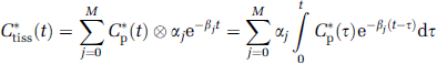
where α
j
and β
j
are assumed to be real-valued and nonnegative. Not all compartmental models satisfy these assumptions, but they are met by the kinetic models used with many PET tracers (Schmidt, 1999) including
From equation (1) one observes that ‘high-frequency’ components (β
j
very large) equilibrate rapidly with and become proportional to Cp
∗
(t), whereas ‘low-frequency’ components (β
j
≅0) are proportional to ∫Cp
∗
(t)dt and account for trapping of tracer. Components with intermediate values of β
j
reflect tissue compartments that exchange material directly or indirectly with plasma; these are referred to as equilibrating components. Noise in the data greatly influences the accuracy with which very low- and high-frequency components can be detected, and the problem is exacerbated when the method is applied where the signal-to-noise ratio is low. In these cases, application of numerical filters becomes essential. Spectral analysis iterative filter, previously developed for estimating rCPS from region-of-interest data (Veronese et al, 2010a), was investigated in the present study for use with voxelwise estimation. Spectral analysis with iterative filter uses a passband filter [βL,βU] to separate trapping and blood components from equilibrating components. The passband lower limit βL represents the smallest exponent β for a component that can be distinguished from trapping of tracer, and the upper limit βU is the largest exponent of a component that can be distinguished from blood in the brain. The passband limits are determined based on prior information on expected tracer kinetics, data sampling schedule, and noise in the data. As in the previous study, we utilized 100 logarithmically distributed values β
j
between 0.0038 and 1.3 min−1 in the estimations (Veronese et al, 2010a). Spectral analysis with iterative filter conserves the main characteristics of spectral analysis—it does not require any prior assumptions concerning number of compartments in the system, and it can be applied to heterogeneous as well as homogeneous tissues. The added benefit of SAIF is that it improves estimates of both α0 and
Leucine Kinetic Model
The model for
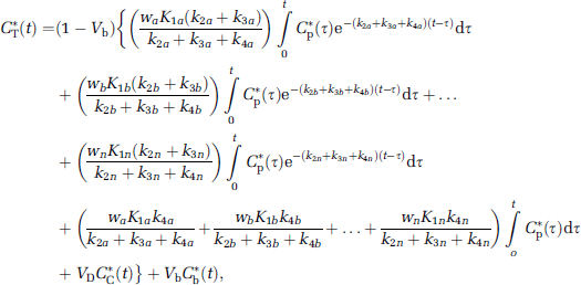
(

When total activity in a brain region or voxel following injection of
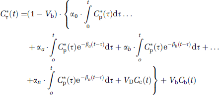
where
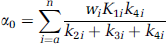
Spectral analysis with iterative filter is used to estimate n and the spectral analysis parameters α0, α
a
, α
b
, …, α
n
, β
a
, β
b
, …, β
n
, and V
b
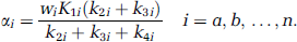
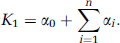
. From these parameters, the leucine parameters of interest can be determined. The latter include the weighted average influx rate constant for the mixed tissue,
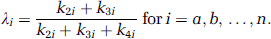
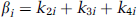
The fraction of unlabeled leucine in the precursor pool for protein synthesis in tissue subregion i that is derived from arterial plasma, λ i ≡(k 2i +k 3i )/(k 2i +k 3i +k 4i ) is identified for each subregion under the constraint that λ a =λ b =…=λ n =λ, as

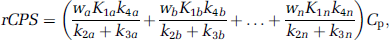
Finally, rCPS in the mixed tissue can be computed as
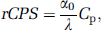
where Cp is the arterial plasma concentration of unlabeled leucine.
Simulation Studies
Simulation 1: Spectral analysis with iterative filter passband: Due to the large discrepancy in signal-to-noise ratio between voxel and ROI TACs, the equilibrating component passband optimized for ROI analysis may not be optimal for voxelwise quantification. To define the passband interval bounds [βL,βU], we followed a simulation strategy similar to that used for application of SAIF at the ROI level (Veronese et al, 2010a). The procedure consisted of simulating noisy voxel-TACs that were subsequently analyzed by SAIF with different passband intervals. The optimal passband was chosen as the one that provided the best trade-off between precision and accuracy of the estimates of rCPS and other parameters of interest.
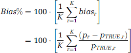
Noise-free voxel-TACs were simulated according to a heterogeneous kinetic model, with two equilibrating components and one trapping component. Model parameters were generated by the random sampling of normal distributions as follow: Vb=0.064±0.009 (unitless), α0=0.012±0.002 (mL g−1 min−1), α1=0.0096±0.0004 (mL g−1 min−1), α2=0.0197±0.0015 (mL g−1 min−1), β0=0 (min−1), β1=0.032±0.004 (min−1), and β2=0.15±0.03 (min−1). These values are the intersubject mean values±s.d. of spectra estimated with ROI-SAIF in whole brain (Veronese et al, 2010a). One thousand noisy TACs were simulated by adding to the noise-free simulated TACs Gaussian noise with zero-mean and variance consistent with the level of noise in voxel data, as estimated in Tomasi et al (2009). Different passband intervals (βL=0.005 to 0.06 min−1; βU=0.1 to 0.6 min−1) were tested. To select the best interval, performance indices percent bias (Bias%) and percent root mean square error (RMSE%) were computed as:
and
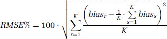
where p r represents the rth SAIF parameter estimate, p TRUE,r indicates the true parameter value for the rth simulated TAC, bias r indicates bias for the rth simulated TAC, and K indicates total number of simulated TACs. Any noise realization that resulted in a negative entry in the simulated TAC was discarded and replaced with a new realization.
Simulation 2: performance of voxelwise spectral analysis with iterative filter: Once the choice of passband was made, a new simulation was performed to quantify the effect of noise on estimated parameters of interest. In these simulations, a bootstrap approach was used as an alternative to random noise generation with a Gaussian model.
To simulate data as close as possible to that measured in a previously acquired PET study, we proceeded as follows:
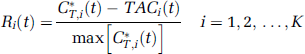
Using the optimal passband interval obtained in Simulation 1, data measured in a representative slice of an individual brain volume, masked to include brain voxels only, were analyzed voxel-by-voxel with SAIF. The set of parameters obtained became the reference, or ‘true,’ parameter values used in the simulations. Outliers and algorithm failures produced at this step were excluded from the simulation. Noise-free TACs were generated by convolving the original measured arterial input function of the subject with the sum of exponential terms defined by the reference parameters from step 1. In addition, for each voxel, normalized residuals R
i
(t) were computed as:
Voxel noise was simulated using a bootstrap approach (Efron, 1979) based on random resampling of normalized residuals. With this approach, noise for the i-th voxel (N
i
(t)) was simulated as
Noisy voxel-TACs were generated by adding the simulated noise to the noise-free TACs as
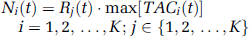

The procedure was repeated 50 times, generating 50 different bootstrap-simulated slices. Note that the bootstrap procedure used here differs from the usual approach of normalizing each residual vector by its standard deviation in order to assure that all resampled residuals have equal variance. In this approach, the required rescaling would be by the standard deviation in the target voxel residual. In the current study, however, we do not have good estimates of the variance in each individual voxel due to the inherent high noise levels of voxel data. Instead, we empirically chose normalization and rescaling to the maxima of the TACs, as these scale factors have the added advantage of preventing negative values in the simulated noisy TACs. The sample variances of the original and bootstrapped residuals were compared to check the effect of the chosen scale factors.
All 50 bootstrap-simulated slices were analyzed with the voxelwise SAIF approach. Spectral analysis with iterative filter applied at the voxel level with the passband interval optimized for voxel analyses will be referred to as voxel-SAIF. We looked at three regions: the whole slice and two ROIs placed on the slice (frontal cortex and corona radiata). As in Simulation 1, to assess the quality of voxel-SAIF results, for each region and each parameter of interest, Bias% and RMSE% were computed. The number of voxels with estimated parameter values considered to be outside the normal physiological range, that is, those with K1>1 mL g−1 min−1, Vb>1, or rCPS>10 nmol g−1 min−1, was recorded (all SAIF parameter estimates are already restricted to be nonnegative by algorithm design), and outlier voxels were excluded from bias and RMSE statistics. For comparison, we also averaged voxel-TACs in each bootstrap-simulated slice over the three regions to obtain ROI TACs, which were then analyzed with SAIF using the passband interval optimized for ROI data (ROI-SAIF) (Veronese et al, 2010a).
We also investigated the capacity of voxel-SAIF to correctly identify the number of kinetic components in each voxel by comparing the number of tissue equilibrating components in the reference data with the number detected in bootstrap-simulated slices.
Positron Emission Tomography Studies
Data from previously reported studies (Bishu et al, 2008, 2009) of six healthy awake male subjects were reanalyzed in the current study. Subject inclusion criteria and the PET study procedure are described in detail in Bishu et al (2008). Briefly, all subjects underwent 90-minute dynamic
The whole brain and 12 regions were evaluated in all subjects. Estimates of Vb, K1, λ, and rCPS were determined in each ROI and in each voxel by using ROI-SAIF and voxel-SAIF, respectively. Weights were inversely proportional to the variance of decay-corrected measured activity in the region, which was modeled assuming Poisson statistics as
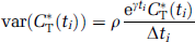
(Wu and Carson, 2002), where γ is the decay constant for 11C, Δt i is length of Frame i, and ρ is a proportionality coefficient reflecting the noise level in the data estimated a posteriori (Veronese et al, 2010a). For voxel-SAIF, weights were based on whole brain activity; in ROI-SAIF, weights were based on activity in the region itself. Tracer arrival delay was calculated as in Veronese et al (2010a).
For all subjects, ROI-SAIF estimates were compared with the mean of voxel-SAIF estimates in all voxels of the region. To assess agreement between methods, we calculated the slope and intercept of the fitted regression line with ROI-SAIF estimates and mean voxel-SAIF estimates in each region and each subject as independent and dependent variables, respectively. Pearson's R2 values were added as correlation measures.
We also visually examined the spatial distribution of voxels found to be kinetically heterogeneous. The ‘heterogeneity map’ was constructed by fusing the MR image with a map of the spatial distribution of voxels with two or more SAIF-estimated equilibrating components.
Results
Simulation 1: Spectral Analysis with Iterative Filter Passband
In simulations performed to find an appropriate filter passband, rCPS bias ranged from 3% to 25%, depending on the cutoff frequencies βL and βU. Root mean square error ranged from 15% to 35% for rCPS estimates, and from 8% to 38% for the other parameters of interest, that is, K1, λ, and Vb. Due to the high level of noise typical of voxel-TACs, these values were much higher than those obtained with ROI-SAIF (bias in rCPS: 0.03% to 7%; RMSE 2.4% to 21.5% (Veronese et al, 2010a)). For voxel-SAIF, we chose 0.02 min−1 and 0.2 min−1 for βL and βU, respectively, as a good compromise between precision and accuracy of rCPS (bias 3%; RMSE 18%) and λ (bias 2%; RMSE 8%). With this passband interval, K1 and Vb displayed, respectively, 8% and 6% bias, and 14% and 28% RMSE. This choice for the voxel-SAIF passband interval differs from that made for ROI-SAIF (βL=0.03 min−1; βU=0.3 min−1) (Veronese et al, 2010a); when the optimal ROI passband was applied to voxelwise analysis bias exceeded 5% for all parameters of interest.
In the following text, voxel-SAIF refers to SAIF applied at voxel level with its optimal passband of [0.02, 0.2] min−1, and ROI-SAIF refers to SAIF applied at the ROI level with its optimal passband interval of [0.03, 0.3] min−1.
Simulation 2: Performance of Voxel-Spectral Analysis with Iterative Filter
Less than 1% of brain voxels in the slice were excluded from the bootstrap simulations due to outlier parameter estimates or failure of the voxel-SAIF algorithm to converge. Table 1 provides results of the bootstrap simulations. Mean values and s.d. of voxel-SAIF bootstrap estimates were in good agreement with parameter mean values and s.d. of the simulated reference values. Bias% and RMSE% of voxel-SAIF estimates for Vb, K1, λ, and rCPS determined in 50 bootstrap simulations for three ROIs are also provided. Bias (<2%) and RMSE (<8%) were both low in estimates of λ. Estimates of rCPS had limited biases (3.9% to 6.0%) and variability consistent with the high level of noise typical of voxel-TACs (RMSE 17.3% to 19.7%). Blood volume, Vb, was also estimated with good accuracy (max Bias% 6.2%) but not high precision (max RMSE% 21.5%), particularly in corona radiata. Similar results were obtained for K1 (max Bias% 9.2%; max RMSE% 12.7%). Normalizing and rescaling led to a small reduction (mean: 5%; range: 0% to 13%) in the standard deviation of the resampled residual values compared to those of the reference data set (see Supplementary Figure).
Performance of SAIF algorithm in bootstrap simulationa
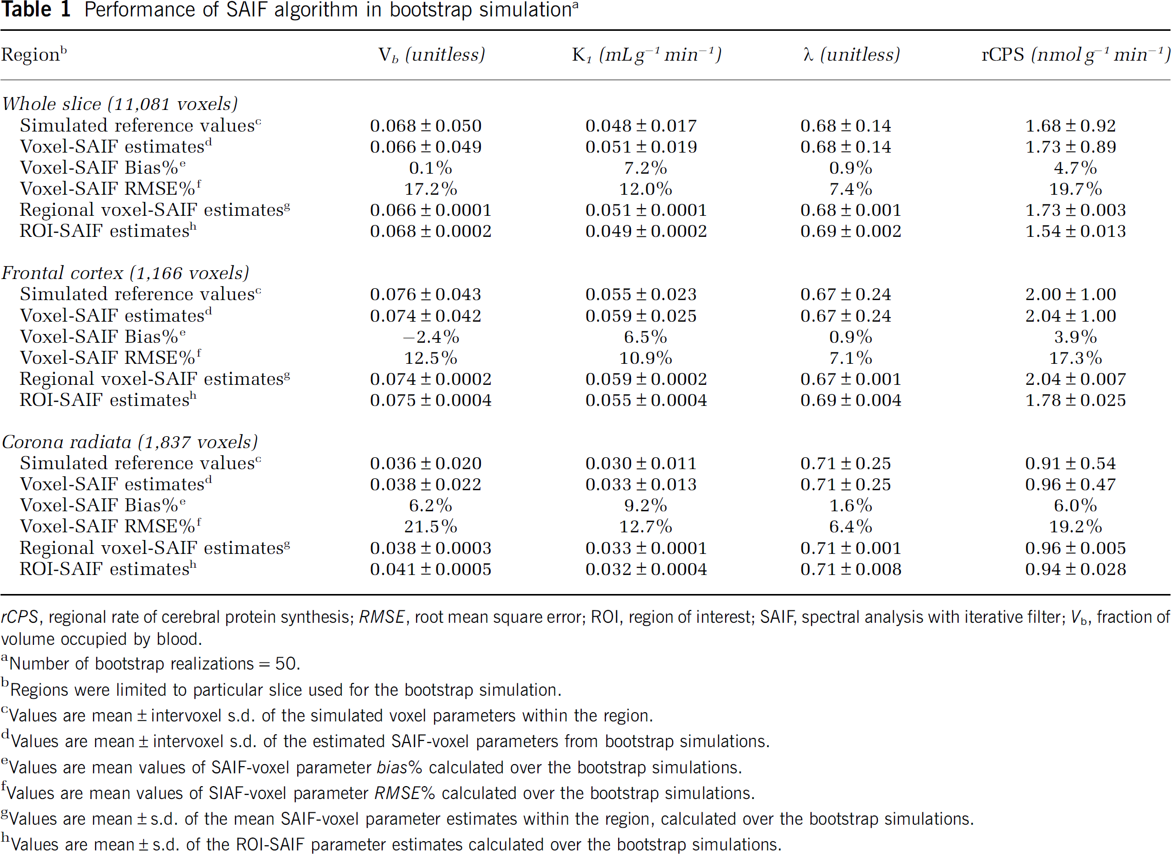
rCPS, regional rate of cerebral protein synthesis; RMSE, root mean square error; ROI, region of interest; SAIF, spectral analysis with iterative filter; Vb, fraction of volume occupied by blood.
Number of bootstrap realizations=50.
Regions were limited to particular slice used for the bootstrap simulation.
Values are mean±intervoxel s.d. of the simulated voxel parameters within the region.
Values are mean±intervoxel s.d. of the estimated SAIF-voxel parameters from bootstrap simulations.
Values are mean values of SAIF-voxel parameter bias% calculated over the bootstrap simulations.
Values are mean values of SIAF-voxel parameter RMSE% calculated over the bootstrap simulations.
Values are mean±s.d. of the mean SAIF-voxel parameter estimates within the region, calculated over the bootstrap simulations.
Values are mean±s.d. of the ROI-SAIF parameter estimates calculated over the bootstrap simulations.
Table 1 also shows comparisons between voxel-SAIF estimates for the parameters, averaged over each ROI, and the corresponding parameters estimated with ROI-SAIF. Estimates of λ, Vb, and K1 show good agreement between voxel and ROI methods. Regional rate of cerebral protein synthesis, which has a small positive bias (6%) when estimated on a voxel-by-voxel basis, is underestimated with ROI-SAIF in the whole slice and frontal cortex by 8% and 11%, respectively. Variability of estimates of λ and rCPS among the 50 bootstrap simulations is lower for the mean of the voxel-SAIF estimates than those determined with ROI-SAIF.
Spectral Analysis with Iterative Filter Application to Measured Positron Emission Tomography Data
In measured PET data, the percentage of voxels in a given ROI in which voxel-SAIF either failed to converge or produced nonphysiological estimates, averaged over all subjects, ranged from 0.7% (Putamen) to 2.9% (Amygdala), depending on the brain area. The mean fraction of outlier voxels over all brain regions was 1.3%, and ∼0.2% of voxels were excluded for failure to converge. The percentage of voxels included in the analysis was >95% for all subjects and regions. In whole brain 0.5% of voxels and in white matter 0.8% of voxels (mean over all subjects) had rates of protein synthesis not detectably different from zero. Figure 2 shows parametric maps for rCPS, λ, and K1 in a representative transaxial slice at level of frontal cortex in one subject. The subject's MRI is also shown. In this slice, rCPS was 1.73±0.96 nmolg−1 min−1 (mean±s.d. over all brain voxels), 5th to 95th percentile range 0.04 to 3.01 nmolg−1 min−1. Regional rate of cerebral protein synthesis shows the well-known pattern with areas of white matter tending to have lower rCPS than gray matter. Voxel-SAIF estimates of λ were 0.68±0.11 (mean±s.d.), corresponding to intraslice variability of ∼16%. Although noisy, the λ image shows a tendency of higher values in white than gray matter areas. The 5th to 95th percentile range of K1 estimates was 0.023 to 0.064 mLg−1 min−1; there is a clear spatial distribution of higher and lower values concentrated in gray and white matter, respectively.
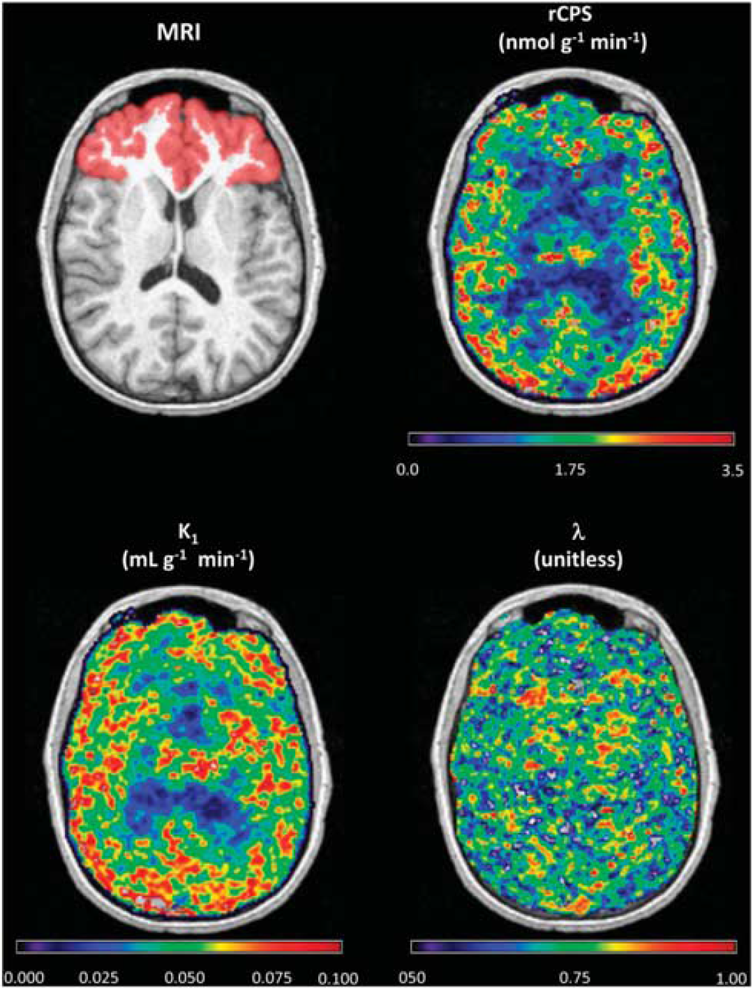
Magnetic resonance imaging (MRI) and parametric maps of regional rate of cerebral protein synthesis (rCPS), λ, and K1 obtained with voxel-spectral analysis with iterative filter (SAIF). Images are of a representative transaxial slice for one subject. Red area in the MRI image represents the frontal cortex region for the particular slice. A Gaussian filter (full width at half maximum (FWHM) 1.7 mm) was employed to smooth each of the parametric images in three dimensions before visualization.
Comparison of Voxel-Spectral Analysis with Iterative Filter and ROI-Spectral Analysis with Iterative Filter in Measured Positron Emission Tomography Data
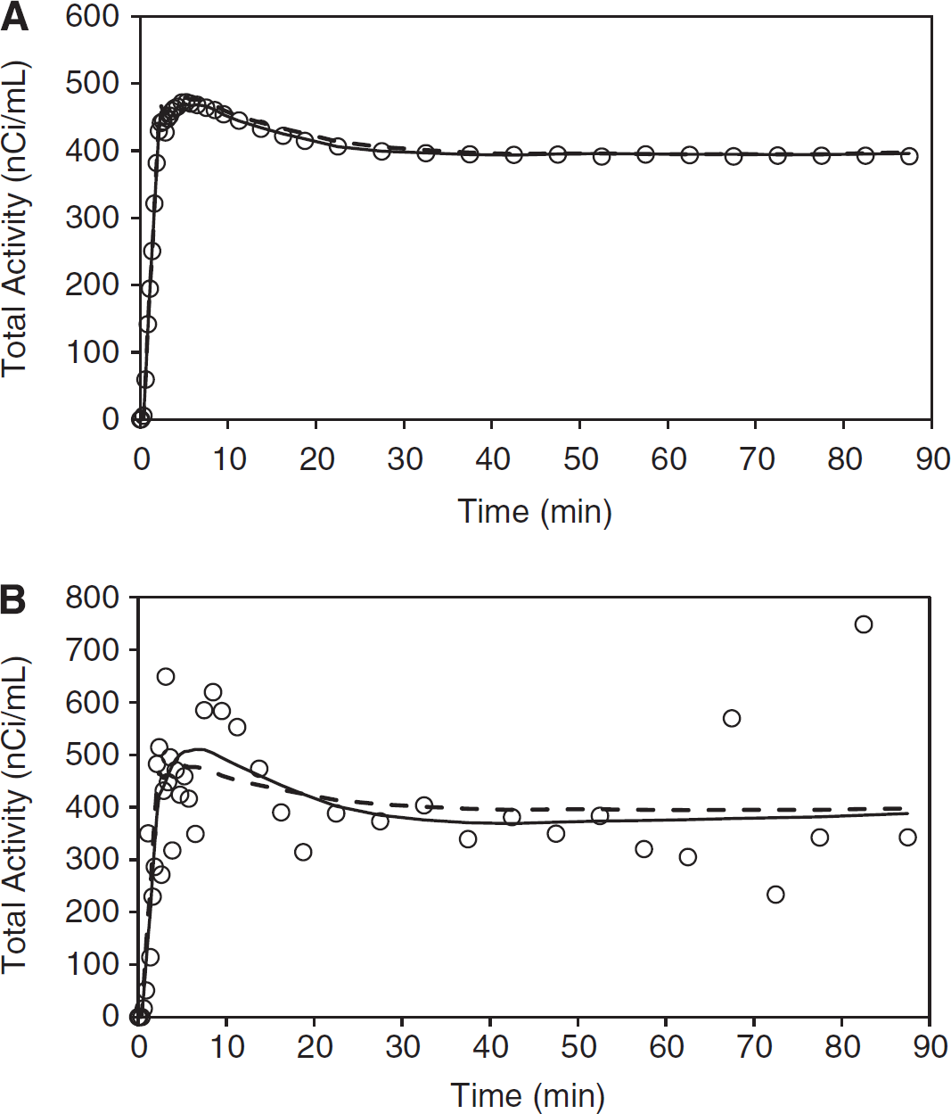
Spectral analysis with iterative filter fits of ROI and voxel-TACs are shown in Figure 3. Overall, good agreement is seen when the mean of voxel-SAIF fits is compared with the ROI-SAIF fit of ROI TAC (Figure 3A). There are, however, small discrepancies: the mean voxel-SAIF fit slightly overestimates the measured activity between ∼2 and 30 minutes, whereas the ROI-SAIF fit has a slight underestimation ∼2 to 8 minutes and a very slight overestimation from ∼15 to 25 minutes. After ∼30 minutes, fits of the two methods are indistinguishable. The measured single voxel-TAC shown in Figure 3B illustrates the very high noise level present in voxel data and the variability between individually fit voxel-TACs (solid line) and the mean of all voxel-TACs in the region (dashed line).
(
Table 2 compares regional mean voxel-SAIF estimates with estimates determined with ROI-SAIF in measured PET data. Mean values and standard deviations for six subjects are reported for 12 ROIs and whole brain. There was excellent agreement between methods in estimates of Vb, K1, and λ; mean relative differences were 1%±4%, −1%±4%, and −2%±2% (mean±s.d. among regions) for Vb, K1, and λ, respectively (Table 2). Except in corona radiata, estimates of rCPS were somewhat higher with voxel-SAIF compared with ROI-SAIF; the mean percent difference between methods ranged from 2% (putamen) to 16% (occipital cortex), with average over all regions ∼7.7%. Differences between voxel- and ROI-SAIF estimates of rCPS tended to be larger in cortical than in subcortical or white matter regions.
Regional estimates of Vb, K1, λ, and rCPSa
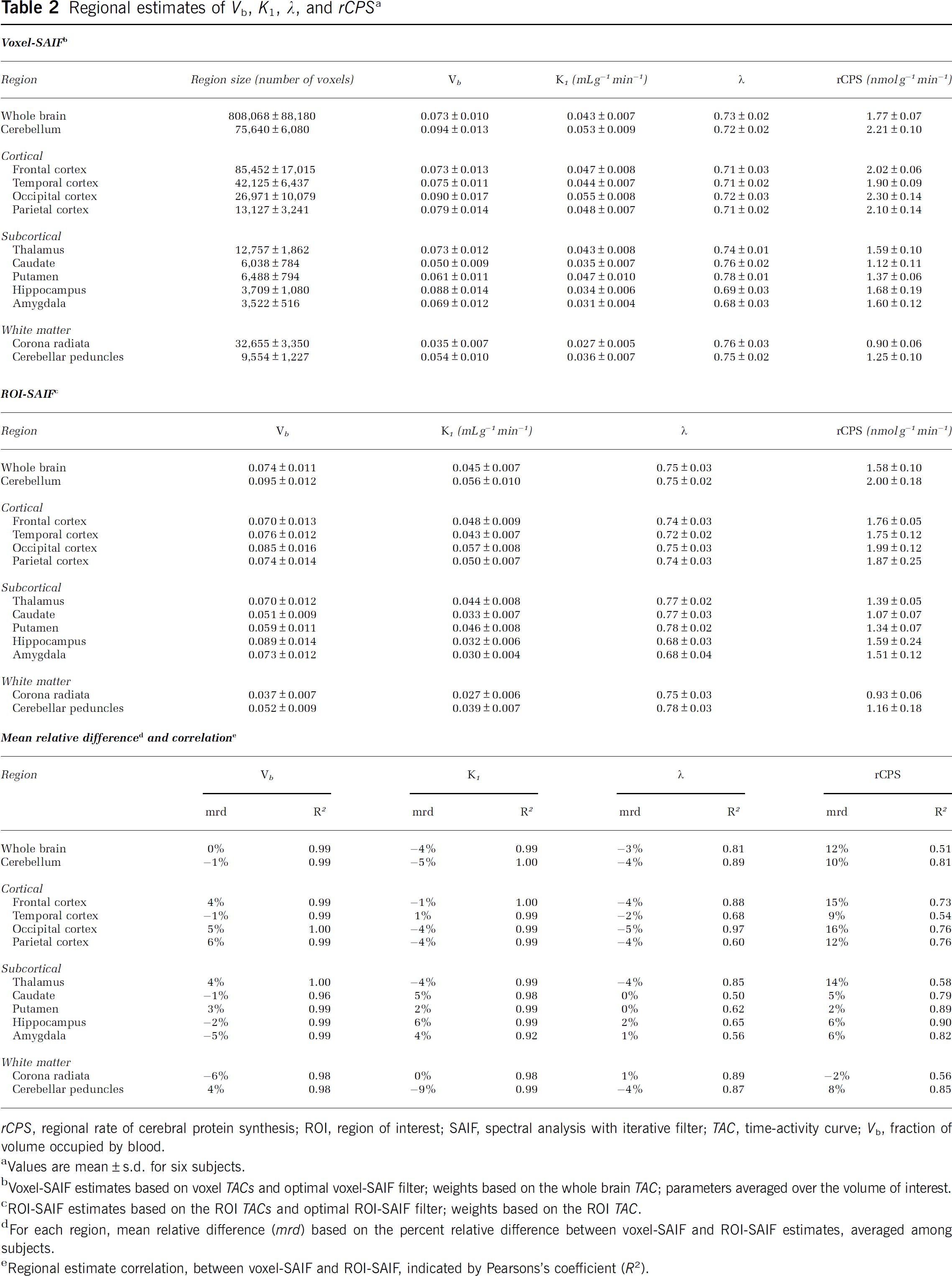
rCPS, regional rate of cerebral protein synthesis; ROI, region of interest; SAIF, spectral analysis with iterative filter; TAC, time-activity curve; Vb, fraction of volume occupied by blood.
Values are mean±s.d. for six subjects.
Voxel-SAIF estimates based on voxel TACs and optimal voxel-SAIF filter; weights based on the whole brain TAC; parameters averaged over the volume of interest.
ROI-SAIF estimates based on the ROI TACs and optimal ROI-SAIF filter; weights based on the ROI TAC.
For each region, mean relative difference (mrd) based on the percent relative difference between voxel-SAIF and ROI-SAIF estimates, averaged among subjects.
Regional estimate correlation, between voxel-SAIF and ROI-SAIF, indicated by Pearsons's coefficient (R2).
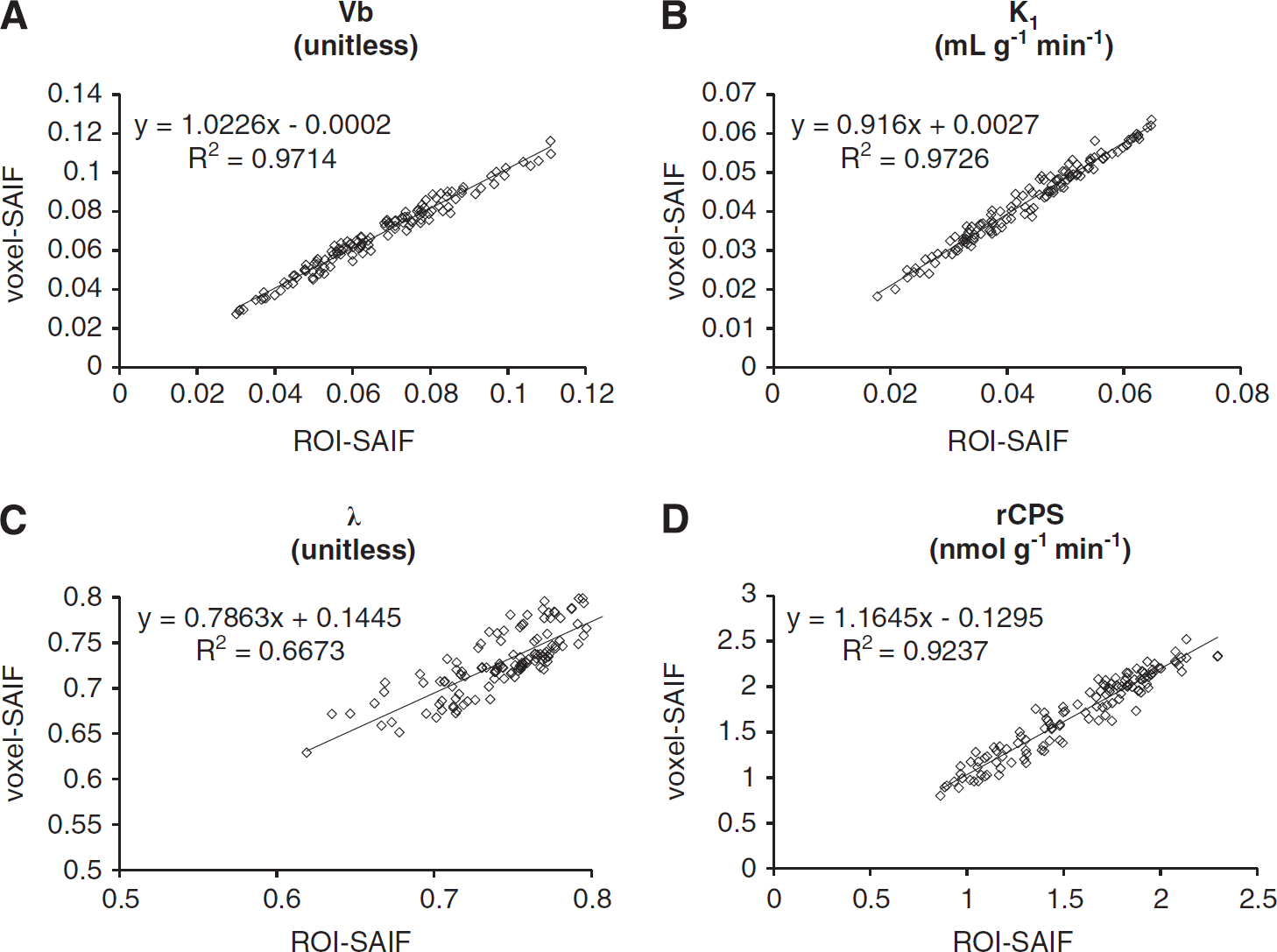
Figure 4 provides scatter plots that compare ROI-SAIF estimates of Vb, K1, λ, and rCPS with voxel-SAIF estimates averaged over the same ROI. All ROIs and all subjects are included. In each plot, the equation of the estimated regression line and Pearson's correlation coefficient are reported. Vb, K1, and rCPS show close correlation between voxel-SAIF and ROI-SAIF estimates (R2>0.92). Estimates of λ are less tightly correlated (R2=0.67).
Scatter plots of regional rate of cerebral protein synthesis (rCPS) (
Heterogeneity Analysis
From analysis of the simulated reference and bootstrap-estimated number of equilibrating components, we evaluated the capacity of voxel-SAIF to correctly determine the number of compartments in the tissue voxel. In 72.3% of voxels, the number of equilibrating components estimated with voxel-SAIF agreed with simulated reference values. In the remaining 27.7%, voxel-SAIF detected a lower (11.4%) or higher (16.3%) number of equilibrating components compared with the reference number. A trapping component was correctly detected in 100% of simulated voxel-TACs.
This behavior is similar to ROI-SAIF performance in simulation, where the accuracy rate for correct determination of number of equilibrating components was 73.1%. In the ROI data, however, ROI-SAIF detected a higher number of equilibrating components in 26% of cases and a lower number in only 1% of regions. As in the voxelwise analysis, a trapping component was correctly detected in all simulated ROIs.
In measured data, differences in the number of detected tissue components were found between the voxelwise and ROI-level analyses, as might be expected. In ROI-SAIF one trapping component, one blood component, and at least two equilibrating components were detected in all regions and subjects. With voxel-SAIF, one trapping and one blood component were found in 100% of successfully estimated voxels, but only 45% of them included two or more equilibrating components. The finding of more than one equilibrating component suggests kinetic heterogeneity of the tissue in these voxels. In the remaining voxels, only one equilibrating component was detected, indicating the homogenous tissue model was appropriate to describe 55% of brain voxel-TACs.
Figure 5 illustrates the spatial distribution of voxels in which two equilibrating components were detected in a representative transaxial slice at the cortical level. From the distribution it appears that the concentration of kinetically inhomogenous voxels is higher at the border between gray and white matter than within the gray or white matter itself. A similar pattern was found in all subjects and brain slices.
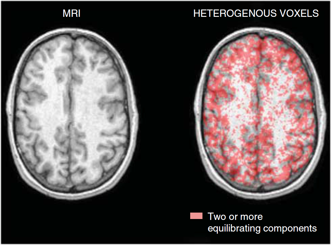
Magnetic resonance imaging (MRI) and spatial distribution of heterogeneous voxels. T1-weighted MR image (left) and the same image fused with the spatial distribution of voxels estimated to be heterogeneous (right). The red area corresponds to those voxels in which voxel-spectral analysis with iterative filter (SAIF) detects two or more equilibrating components.
Discussion
Before this study, voxelwise estimation of kinetic model parameters of
Setting the passband filter limits and assessing performance of SAIF at the voxel level was carried out in two simulations that used different noise generation methods. To be consistent with the strategy defined in Veronese et al (2010a) for selection of the passband, we used a Monte Carlo approach, a standard method for noise generation in simulation, widely used and easy to implement. Due to the high noise levels, however, the Monte Carlo approach led to simulated TACs in some voxels with negative activity values. To avoid negative activities in simulated TACs, we utilized bootstrapping of residuals for noise generation in the simulation to assess performance of voxel-SAIF. Negative entries in simulated TACs were avoided by normalizing reference residuals and rescaling the resampled residuals by the maxima of the associated TACs; this choice of scale factors had only a modest effect on noise variance. Results of the two types of simulation were consistent: performance indices for rCPS and other parameters were comparable. Of note, in addition to the assumption of equal residual variances discussed previously, the bootstrap approach assumes that residuals have zero-mean and are statistically independent. The zero-mean assumption was easy to verify (mean of voxel residuals: −0.002 nCi/mL). The statistical independence assumption is known to be incompletely met for voxel data: the process of PET data reconstruction leads to spatial correlation between nearby voxels, although correlation drops off rapidly as distance between voxels increases (Pajevic et al, 1998). Accounting for spatial correlation is a difficult statistical problem beyond the scope of the present study. Methods that perform kinetic modeling in a transformed space, for example, in the wavelet domain, can account for spatial correlation in the data, but apply only to models in which the estimation operator is linear in the data, such as a Patlak plot or Logan analysis (Turkheimer et al, 2000). Further investigation is needed to determine the performance of these methods with voxel-SAIF analysis. We utilized here the routinely used approach that treats each voxel-TAC as independent from the others.
One remarkable outcome of the analysis was the good performance of voxel-SAIF in estimation of leucine kinetic parameters and rCPS. When simulated reference values were compared with bootstrap-estimated parameters, voxel-SAIF demonstrated low bias and good precision. Moreover, voxel-SAIF produced a low number of outliers. Essential to the performance of voxel-SAIF was selection of an appropriate passband whose role is to reduce the influence of noise on parameter estimates. The optimal voxel-SAIF passband filter differed somewhat from that used for ROI-SAIF. In particular, high-frequency noise present in voxel data but attenuated in the ROI data reduces the accuracy with which high-frequency components can be estimated. The upper bound for the voxel-SAIF passband filter was more selective compared to the filter for ROI-SAIF (0.2 min−1 instead of 0.3 min−1); this reduces the impact of high-frequency noise. At the other end of the spectrum, the less restrictive lower bound of the voxel-SAIF passband (0.02 min−1 for voxel-SAIF; 0.03 min−1 for ROI-SAIF) has the effect of allowing greater kinetic variability in low-frequency components among individual brain voxels.
In measured data, when means of voxel-SAIF estimates within a region were compared with ROI-SAIF estimates, there was generally good agreement between analysis methods. Unlike fixed compartmental model analyses, spectral analysis allows the tissue ROI to be represented as a linear combination of any number of tissue compartments. Because the tissue ROI could be represented as a linear combination of the compartments of each voxel comprising the ROI, we could expect good agreement between the ROI-SAIF estimates and mean voxel-SAIF estimates of linear parameters of the model. Indeed, the linear parameter Vb and the parameter K1, which is the sum of the linear coefficients α i , exhibit the best agreement (1%±4% and 1%±4%, mean±s.d. of the difference between ROI-SAIF and mean voxel-SAIF estimates of Vb and K1, respectively) and highest correlation between methods (0.97 for both Vb and K1).
In contrast to linear parameters, λ and rCPS are nonlinear combinations of parameters, and therefore less agreement between ROI-SAIF and mean voxel-SAIF estimates is to be expected. Estimates of λ were 2%±2% higher with ROI-SAIF and correlation between estimates provided by the two methods was 0.67. Correlation between rCPS estimated with the two methods was very high (R2=0.92), but estimates were 8%±6% lower with ROI-SAIF. Determination of λ from the SAIF-estimated coefficients α i is based on the assumption that all λ in the subregions of a heterogeneous tissue are equal; this constraint is likely to have a greater impact when data are analyzed at the ROI level, where a uniform value of λ for the entire region is assumed, than when data are analyzed at the voxel level and λ can vary among voxels within the region. The constraint contributes to differences between ROI-SAIF and voxel-SAIF estimates of λ and, by extension (equation), estimates of rCPS.
Spectral analysis can also be used to provide information on number of compartments in the kinetic model of the tracer in tissue. For the tracer
Analysis of the spatial maps of heterogeneous voxels, in which voxel-SAIF selected the heterogeneous kinetic model to describe the voxel-TACs, suggests the presence of a distribution pattern: in our scans heterogeneous voxels appear to be concentrated at the borders between gray and white matter. This finding was somewhat surprising; we had expected more gray matter voxels to be considered heterogeneous due to inherent gray matter heterogeneity, for example, differences in rCPS among the cortical layers, and partial volume effects arising from the limited spatial resolution of the scanner. The partial volume effects would be greater, and therefore more voxels may be considered as heterogeneous, in lower-resolution scans. The present results do, however, confirm that use of a homogenous kinetic model to describe voxel-TACs is not appropriate for all voxels in brain, even on a high-resolution scanner.
Use of the iterative filter implemented in SAIF improved the robustness of the method to noise; voxel-SAIF provided good estimates of leucine kinetic parameters and rCPS, even at high noise levels. Region-of-interest-based- and mean voxel-based-rCPS estimates were highly correlated, but ROI-based estimates were higher. Simulations showed that mean voxel-level rCPS estimates had lower bias than ROI-based estimates in whole brain and cortex, had comparable bias in white matter, and had lower variability in all regions. We conclude that estimation of rCPS with SAIF is improved when the method is applied at the voxel level. Voxel-SAIF may also provide useful information about the spatial distribution of voxel heterogeneity.
Footnotes
References
Supplementary Material
Please find the following supplemental material available below.
For Open Access articles published under a Creative Commons License, all supplemental material carries the same license as the article it is associated with.
For non-Open Access articles published, all supplemental material carries a non-exclusive license, and permission requests for re-use of supplemental material or any part of supplemental material shall be sent directly to the copyright owner as specified in the copyright notice associated with the article.