Sage Journals: Discover world-class research

Abstract

At its most fundamental level, cerebral blood flow (CBF) may be modeled as fluid flow driven through a network of resistors by pressure gradients. The composition of the blood as well as the cross-sectional area and length of a vessel are the major determinants of its resistance to flow. Here, we introduce a vascular graph modeling framework based on these principles that can compute blood pressure, flow and scalar transport in realistic vascular networks. By embedding the network in a computational grid representative of brain tissue, the interaction between the two compartments can be captured in a truly three-dimensional manner and may be applied, among others, to simulate oxygen extraction from the vessels. Moreover, we have devised an upscaling algorithm that significantly reduces the computational expense and eliminates the need for detailed knowledge on the topology of the capillary bed. The vascular graph framework has been applied to investigate the effect of local vascular dilation and occlusion on the flow in the surrounding network.

Keywords

CBF ischemia modeling oxygen transport

Introduction

Cerebral blood flow (CBF) is dynamically regulated to ensure that supply and current metabolic demand are always in balance, as has been discovered more than hundred years ago (Mosso, 1881; Roy and Sherrington, 1890). More recently, imaging modalities have been developed that use CBF as a surrogate of neural activity for functional mapping (Ogawa et al, 1990; Kwong et al, 1992). However, several studies have shown that neurovascular coupling is a nonlinear phenomenon, and the spatial specificity of the hemodynamic response, as well as the complex interplay of the diverse CBF regulating mechanisms remain largely unknown (Turner, 2002). Furthermore, the current state of the art blood flow imaging modalities are either limited to a small field of view or have a low spatial and/or temporal resolution.

As computational modeling of CBF does not suffer from these limitations, it has become an important research supplement and provides a means to test hypotheses in ways that are not possible in experimental investigations.

A large fraction of the earlier proposed models is devoted to describing and predicting the outcomes of specific CBF measurement modalities, such as arterial spin labeling (Buxton et al, 1998; Parkes and Tofts, 2002; Zhou et al, 2001). The more general models that have been introduced, either make highly simplified approximations of the angioarchitecture or focus on a small fraction of the cerebral vasculature only, for example, the microvascular network (Tsoukias et al, 2007) or large vascular structures, such as the Circle of Willis (Castro et al, 2006).

Boas et al have recently presented a framework that is restricted neither to a specific imaging method nor to a particular fraction of the vasculature (Boas et al, 2008). Their aim, as stated in the paper, is to develop the simplest model possible that can accurately predict the dynamic behavior of the complex vascular system.

Our vascular graph (VG) model, developed in parallel, makes use of the same underlying principles and governing equations, but our focus lies on the framework's applicability to realistic vascular networks, for example, obtained by high-resolution angiography methods. We significantly extend the model's capabilities in this respect by introducing upscaling algorithms that allow working with integral quantities of the capillary bed, rather than with its discrete representation. This drastically reduces the computational cost and also becomes very beneficial when the discrete capillary topology is unknown.

Moreover, we have included the notion of a three-dimensional tissue representation that is coupled to the vascular network. The solution of the advection and diffusion equations in combination with an exchange term makes it possible to model the three-dimensional scalar transport in both vasculature and tissue and the transfer of the scalar between the compartments.

The model properties of individual blood vessels, such as their diameter, may be manipulated easily. This allows investigating how local dilations or constrictions influence the blood flow in the surrounding tissue. Among others, this is relevant for the earlier addressed issue of the hemodynamic response to neural activity, as well as for the study of cerebrovascular pathologies.

Materials and methods

Basic Model Concepts

The principal idea of our VG model is to represent the cerebral vasculature by a graph, i.e., a collection of vertices or ‘nodes’ and an ensemble of edges that connect pairs of nodes. In such a VG, nodes represent locations in which vessels bifurcate or end, and edges designate the vessels themselves. In graph-theory terminology, the cerebral vasculature can be called a multigraph because two vertices may be connected by more than one edge.

The graph data structure provides an easy handle to compute CBF. If two adjacent nodes (nodes that share a common edge) are at different blood pressure values, this will elicit a blood flow in the vessels that connect them. The magnitude of the flow will depend on the pressure difference and the conductance of the vessels. If we further require that mass is conserved at each node, we can solve the resulting system of equations to yield pressure and flow values for the entire graph (given appropriate boundary conditions). This procedure has been thoroughly described for the analogous problem in electrical circuits (Weinberg, 1962), in which it is referred to as node voltage analysis. Lipowsky and Zweifach have adapted the method to vascular networks (Lipowsky, 1974 and Zweifach, 1974). In the following, we will further extend the model along the lines of Boas et al (2008), but with special focus on three-dimensionality and application to complex realistic vascular networks.

Model Network Construction

Throughout this paper, we have used graph representations of the rat cerebral vasculature to illustrate the capabilities of the VG modeling framework. The following listing provides an overview of the steps involved to generate these VGs:

Perfuse deeply anesthetized rats with phosphate buffered saline, followed by barium sulfate.

Remove brains and punch out cortex samples.

Perform X-ray tomographic microscopy of the samples to yield stacks of transversal grayscale images (slices).

Use custom software to correct images for artifacts and incomplete filling of the vessels with X-ray absorber.

Use propriety software to extract vessel midlines from the image stacks, detect branch and end points and assign a radius value to each midline voxel.

Replace tortuous midlines between branchpoints by straight edges, each of which is associated with a representative mean diameter (i.e., cylinders).

Identify large arteries and veins and set appropriate pressure boundary conditions at the corresponding graph nodes.

Use VG model to solve for pressure, blood flow, and scalar transport (e.g., oxygen transport) in the entire sample domain.

Each point will be discussed in more detail in the subsequent paragraphs. Note that the VG model is a general framework that can be applied to many kinds of angiography data and is not limited to the procedures described here.

Synchrotron Radiation Based X-Ray Tomographic Microscopy (srXTM) of Brain Vasculature

Deeply anesthetized rats were transcardially perfused with heparinized phosphate buffered saline followed by 4% paraformaldehyde. Then, a dispersed suspension of BaSO₄ (Sachtleben GmbH, Duisburg, Germany, 500 mg mL⁻¹ containing 3% bovine gelatin) was injected. After removal of the brain, cylindrical samples of approximately 2.8 mm³ from the somatosensory cortex were punched out and embedded in EPON (Plouraboue et al, 2004). The samples were then scanned at the TOMCAT beamline at the Swiss Light Source. Absorption-based srXTM was performed using monochromatic X-rays with a beam energy set to 20 keV to maximize absorption contrast and to provide sufficient photon flux to penetrate the large sample. The optical magnification was 20 x, resulting in isotropic voxels of 700 nm for the reconstructed images.

Vascular Network Generation from srXTM Images

For each sample, the reconstructed srXTM grayscale images (typically 4000 2DTiff images, 2048 × 2048 pixels each) were cropped and segmented using custom Matlab routines (Matlab, Mathworks, Natick, MA, USA). From the resulting binary images, the three-dimensional VG was extracted using Amira (Visage Imaging GmbH, Berlin, Germany). This involves extracting the midlines of the blood vessels by a morphologic erosion procedure as well as detection of the branch and end points of the thinned vessels. Each midline voxel is associated with a vessel radius value, computed from the binarized images.

Conceptually, the midlines connecting branch points (or branch and end points) represent the edges of the VG. To reduce the computational cost of both VG model simulations and visualizations, the tortuous midlines are replaced by straight edges. Each edge is assigned a radius value, which is the mean of the radii associated with the corresponding midline voxels. Consequently, the graphical representation of an edge is a cylinder with a radius equal to the assigned mean radius. Figure 1 illustrates this transition of srXTM data to the VG representation.

Figure 1

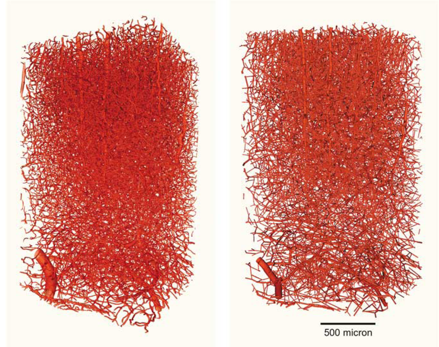
The left image depicts synchrotron radiation based X-ray tomographic microscopy data of rat somatosensory cortex. Details of the data acquisition methodology can be found in Plouraboue et al, Heinzer et al, Stampanoni et al. To the right, the representation of the microscopy data in the vascular graph model is shown. The tortuous vessel parts between bifurcation or end points are replaced by straight connections, i.e., cylinders with a radius corresponding to the mean radius of the vessel.

Finally, the radii of all edges were scaled such that a mean capillary size of 6 μm was reached yielding a vascular volume fraction of 2.52%. This step is necessary to account for shrinkage of the perfused brain tissue during the preparation process.

Classification of Large Vessels

Large vessels were classified as either arteries or veins, based on the results of a pairwise connectivity analysis. Vessels that connect strongly to each other were assigned the same category, based on the fact that there exist no arteriovenous shunts in healthy brain tissue (e.g., Duvernoy et al, 1981). The vessel groups were identified as arteries or veins based on various topological criteria. Generally, veins have a larger diameter than arteries and they have more numerous daughter vessels that branch off at comparably blunt angles. The ratio of arteries to veins was 1.55:1, closely matching our earlier findings in vascular corrosion casts of macaque visual cortex (Weber et al, 2008). Diameter-dependent pressure boundary conditions were set at the feeding vessel's entry/draining vessel's exit points. Pressure values were taken from literature (Zweifach, 1974).

Governing Equations

As described above, every edge in the VG designates a cerebral blood vessel. In general, these vessels are tortuous and their cross-sectional area varies along their length. For simplicity, our VG model approximates each vessel by a straight cylinder of the same length as its real, tortuous counterpart. The variations in cross-sectional area are approximated by a mean value. This model can be refined to arbitrary precision by introducing additional vertices and edges along each vessel, but the following consideration will show that this is not necessary.

The Reynolds number of fluid flow in a cylinder is defined as

R e = \frac{u D}{v},

(1)

where u is the velocity of the fluid, v its kinematic viscosity, and D the diameter of the cylinder. Schaffer and coworkers have measured blood flow velocities in cortical vessels that derive from the middle cerebral artery, as well as in penetrating arterioles, using two-photon imaging (Schaffer et al, 2006). Their results confirm that Re≤2 for all but the largest vessels in the brain. As a consequence, inertial effects play an insignificant role, and the cross-sectional velocity profile remains stable even for curved paths. Therefore, our straight cylinder-approximation exhibits the same flow properties as the real, tortuous network.

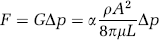
Every node is associated with a blood pressure value. Differences in pressure between adjacent nodes drive the flow of blood through the vessels connecting them. The conductance G of such a vessel (i.e., the inverse of its resistance R to flow) is modeled as

G = α \frac{ρ A^{2}}{8 π μ L}

(2)

Here, A, L, μ, and ρ are the cross-sectional area and length of the vessel, the dynamic viscosity and blood density, respectively. The blood viscosity is known to vary with vessel diameter and hematocrit and thus has to be determined for each vessel individually. Lipowsky and collaborators have derived an empirical equation for the relative apparent viscosity as a function of hematocrit, based on an impressive collection of experimental data by multiple research groups (Lipowsky et al, 1980). To evaluate this expression for each vessel, we require the local hematocrit. Values were taken from the work of Pries and collaborators, who have measured microvessel hematocrit for a wide range of vessel diameters (Pries et al, 1992).

For α = 1, Equation (2) represents the conductance consistent with Hagen-Poiseuille flow through a perfect cylindrical vessel. Deviations of α from one (i.e., α < 1) account for departures from that geometrical idealization. In the current studies, α was set equal to one everywhere.

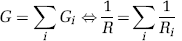
If two adjacent vertices are connected by more than one edge, the effective conductance between the nodes is the sum of the individual vessel conductances (analogous to parallel resistors in an electrical circuit):

G = \sum_{i} G_{i} \Leftrightarrow \frac{1}{R} = \sum_{i} \frac{1}{R_{i}}

(3)

The mass flow rate

F = G Δ p = α \frac{ρ A^{2}}{8 π μ L} Δ p

(4)

through a vessel is the product of its conductance and the pressure difference Δp across its length. This linear relationship between pressure drop and mass flow rate holds even for tortuous vessels with noncircular cross-sections, as long as the local velocity profiles remain self-similar for varying flow rates, and deviations from Hagen-Poiseuille flow can be characterized by the scaling factor α. Because of the existence of blood cells, bifurcations cause an additional resistance to flow, but currently this rheological effect is not modeled; our angiography data, however, provides the necessary information for future improvements.

The continuity equation states that the net mass flow through every node i must match the local accumulation rate, unless the node is a sink or a source, in which case

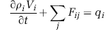
\frac{\partial ρ_{i} V_{i}}{\partial t} + \sum_{j} F_{i j} = q_{i}

(5)

where V_i is the volume associated to node i, and F_ij are the flows to the neighboring nodes j. Cross-sectional area and length of the vessel i—j are denoted as A_ij and L_ij, respectively. Moreover, q_i and ρ_i are the source term and blood density at node i. In our simulations, we assume that blood density is constant throughout.

The node volume in Equation (5) is computed from the node's adjoining vessels as

V i = \frac{1}{2} \sum_{j} A_{i j} L_{i j}

(6)

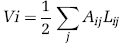
The factor 1/2 is due to the fact that we assign half the volume of an edge to each of its two vertices.

Computation of Pressure and Mass Flow

By substituting Equation (4) into Equation (5) one obtains

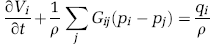
\frac{\partial V_{i}}{\partial t} + \frac{1}{ρ} \sum_{j} G_{i j} (p_{i} - p_{j}) = \frac{q_{i}}{ρ}

(7)

for each node i, where G_ij = G_ji is the conductance of the edge connecting nodes i and j. Note that the first term of Equation (7) vanishes for rigid vascular networks (i.e., inelastic vessels).

To calculate the pressure values p = (p₁,…,p_n)^T at all bifurcation points, the sparse linear system

M \cdot p = q

(8)

has to be solved, where each line represents an equation of the form (7), and the boundary conditions have to be set appropriately.

The continuity equation has a nonzero right-hand side at those nodes where arteries enter or veins leave the computational domain. At these locations one can set rate boundary conditions by supplying a value for q. However, often pressure values are more readily available than flow rates in which case it is more desirable to set pressure boundary conditions instead. Note that the contribution from the nodes with fixed pressure values appear on the right hand side of Equation (8).

Currently, we use the Gauss—Seidel algorithm to solve the linear system (8), but more advanced sparse linear system solvers, such as algebraic multigrid methods, can be implemented in the future.

Once the pressures have been computed using the above protocol, the local mass flow can be calculated according to Equation (4).

Elasticity

The diameter of venules and capillaries may vary dynamically with the transmural pressure. Our VG model captures this effect by making the cross-sectional area, and consequently the vessel volume, pressure dependent. Equation (7) is discretized by approximating the partial derivative ∂V_i/∂t with

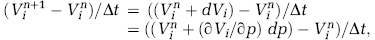
\begin{aligned} (V_{i}^{n + 1} - V_{i}^{n}) / Δ t & = ((V_{i}^{n} + d V_{i}) - V_{i}^{n}) / Δ t \\ = ((V_{i}^{n} + (\partial V_{i} / \partial p) d p) - V_{i}^{n}) / Δ t, \end{aligned}

where the superscript n denotes the time step. As the change in cross-sectional area of a vessel ij depends on the pressure of both nodes i and j, the corresponding change in vascular volume associated with node i may be described by

d V_{i} = 1 / 2 \sum_{j} L_{i j} / 2 ((\partial A_{i j} / \partial p_{i}) d p_{i} + (\partial A_{i j} / \partial p_{j}) d p_{j}) .

Thus, we finally arrive at

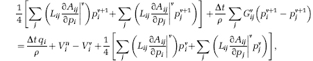
\begin{aligned} \frac{1}{4} [\sum_{j} (L_{i j} {\frac{\partial A_{i j}}{\partial p_{i}} ǀ}^{v}) p_{i}^{v + 1} + \sum_{j} (L_{i j} {\frac{\partial A_{i j}}{\partial p_{j}} ǀ}^{v} p_{j}^{v + 1})] + \frac{Δ t}{ρ} \sum_{j} G_{i j}^{v} (p_{i}^{v + 1} - p_{j}^{v + 1}) \\ = \frac{Δ t q_{i}}{ρ} + V_{i}^{n} - V_{i}^{v} + \frac{1}{4} [\sum_{j} (L_{i j} {\frac{\partial A_{i j}}{\partial p_{i}} ǀ}^{v}) p_{i}^{v} + \sum_{j} (L_{i j} {\frac{\partial A_{i j}}{\partial p_{j}} ǀ}^{v} p_{j}^{v})], \end{aligned}

(9)

where the superscripts v and v + 1 denote quantities at the old and new iteration levels, respectively.

Note that $\partial A_{i j} / \partial_{p_{i}} ǀ^{v}, \partial A_{i j} / \partial_{p_{j}} ǀ^{v}, V_{i}^{v}$ , and $G_{i j}^{v}$ are updated iteratively, such that on convergence $V_{i j}^{v + 1} = V_{i}^{v}$ and $G_{i j}^{v + 1} = G_{i j}^{v}$ are the values $V_{i}^{n + 1}$ and $G_{i j}^{n + 1}$ at the new time level.

In our simulations, we have used the pressure-volume relation proposed by Mandeville et al (1999) to obtain values for ∂A/∂p, but any desired vessel compliance may be implemented.

Upscaling of the Fine-Scale Vascular Structures

Because of rising computational complexity, it may not be feasible to fully resolve large vascular systems. Therefore, while it is important (and inexpensive) to preserve the discrete topology of the large vessels, it may be preferable to model the small vascular structures with an upscaling approach.

Here, we propose a procedure in which the domain is divided into a number of sub-volumes (cells). For each of these cells, integral quantities such as effective conductance, vascular volume, and surface area are determined and a single upscaled vertex replaces all capillary vertices that the cell comprises.

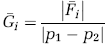
To compute the conductance of a cell i between two of its faces, the vasculature of that cell is studied in isolation. The end nodes of all capillaries crossing the first face are set to an arbitrary fixed pressure p₁, and the end nodes of all capillaries crossing the second face are set to a pressure p₂ ≠ p₁. All capillaries crossing the other boundaries are assumed to be impermeable. The integral mass flow Ϝ̄_i is computed for this configuration and the effective conductance of that cell in the corresponding direction becomes

{\bar{G}}_{i} = \frac{ǀ {\bar{F}}_{i} ǀ}{ǀ p_{1} - p_{2} ǀ}

(10)

For our simulations we have chosen cubic cells, each of which is connected to its six nearest neighbors. The conductance calculation therefore needs to be executed three times per cell, once for every spatial direction. The concept is illustrated in Figure 2. The conductance of the connection between two upscaled vertices can be calculated by computing the harmonic average of the conductances of the two individual cells in the direction of their connection (Figure 2, right).

Figure 2

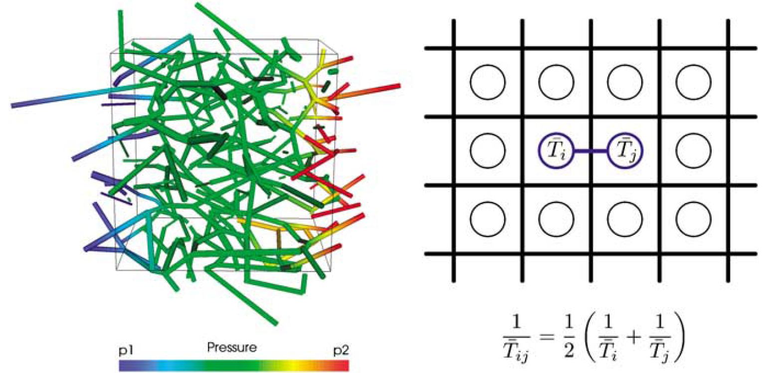
Left: The conductance of a cell in a specific direction can be computed by setting the capillaries crossing the corresponding faces to arbitrary, unequal, fixed pressure levels. The linear system is solved and the mass flow computed. The quotient of mass flow and pressure difference equates to the conductance of the cell in the given direction. Right: The effective conductance of a connection between two cell nodes is given by the harmonic average of the two corresponding conductances, analogous to the sum of resistances of serial resistors. The division by two is due to the fact that only half the cell side-length of each cell needs to be considered.

In order for this upscaling algorithm to succeed, the cell size needs to be chosen sufficiently big (e.g., cell side length bigger than twice the maximum capillary length). Algorithmically, flow computations using the upscaled network are equivalent to the fully resolved case. The only difference is the discretization of the accumulation term, where only the local cell pressure value is involved. The resulting discretization for the balance in cell i reads

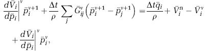
\begin{aligned} {\frac{d {\bar{V}}_{i}}{d {\bar{p}}_{i}} ǀ}^{v} {\bar{p}}_{i}^{v + 1} + \frac{Δ t}{ρ} \sum_{j} {\bar{G}}_{i j}^{v} ({\bar{p}}_{i}^{v + 1} - {\bar{p}}_{j}^{v + 1}) = \frac{Δ t {\bar{q}}_{i}}{ρ} + {\bar{V}}_{i}^{n} - {\bar{V}}_{i}^{v} \\ + {\frac{d {\bar{V}}_{i}}{d {\bar{p}}_{i}} ǀ}^{v} {\bar{p}}_{i}^{v}, \end{aligned}

(11)

where ̄p_i, ̄p_j, ̄q_i, ̄V_i, and d̄VB_i/d̄p_i are effective pressure, source term, integral capillary volume, and its sensitivity to ̄p_i, respectively. Otherwise, the same solution algorithm can be applied.

The connection between the fully resolved and the upscaled system is established by connecting each precapillary or postcapillary end node of the resolved structure with the respective cell-node of the upscaled capillary network.

Scalar Transport

In passive scalar transport, a given concentration distribution (determined by the initial boundary condition) changes over time, as the scalar is advected with the flow (examples being drug or heat transport within the vasculature). To capture the advection process, the discretized scalar transport equation

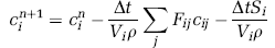
c_{i}^{n + 1} = c_{i}^{n} - \frac{Δ t}{V_{i} ρ} \sum_{j} F_{i j} c_{i j} - \frac{Δ t S_{i}}{V_{i} ρ}

(12)

needs to be solved, where S denotes the rate of scalar diffusion into the surrounding tissue. The superscripts denote the individual time steps, whereas the subscripts designate the node index. This expression may be used for both resolved and upscaled networks. In the upscaled case, however, analogous to Equation (11), F_ij, V_i, S_i, and c_i have to be replaced by ̄F_ij, ̄V_i, ̄S_i, and ̄c_i, respectively. Note that ̄S_i is the integral transfer rate through the vessel walls in cell i, and ̄c_i is the mean concentration. For the evaluation of C_ij a simple upwind scheme based on the mass flow F_ij is used.

Within the tissue, the evolution of the scalar concentration C is described by the conservation law

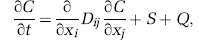
\frac{\partial C}{\partial t} = \frac{\partial}{\partial x_{i}} D_{i j} \frac{\partial C}{\partial x_{j}} + S + Q,

(13)

where D_ij is a diffusion tensor, S the source describing the exchange with the vascular network, and Q a source term representing additional interactions, for example, oxidative metabolism.

The tissue continuum can be approximated by a graph that is analogous to the upscaled graph discussed above. It consists of interconnected nodes, each of which represents a (tissue-) volume and stores numerical quantities, such as the scalar concentration in that volume. For simplicity, we have chosen an isotropic cubic lattice, but any desired topology may be implemented. Whenever a vessel passes through a tissue cell, the associated tissue node appears in the sink term of the corresponding vascular nodes', transport Equation (12), and the vascular nodes act as sources for the tissue node in Equation (13).

The form of coupling between tissue and vasculature is dictated by the physiology. To current knowledge, it can be assumed that S depends on the vascular surface area and the concentration difference c_i-C_i. Thus, S_i in Equation (12) can be expressed as

S_{i} = [\frac{ρ}{2} \sum_{j} A_{i j} Γ_{i j}] (c_{i} - C_{i}),

(14)

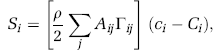
where Γ_ij is the transfer coefficient for the vessel i-j. Similarly, the integral transfer rate for an upscaled cell i reads

{\bar{S}}_{i} = ρ {\bar{A}}_{i} {\bar{Γ}}_{i} ({\bar{c}}_{i} - C_{i}),

(15)

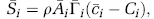
where ̄A_i is the total capillary surface area, Γ̄_i the effective transfer coefficient and ̄c_i the average concentration in the cell volume. Note that the algorithm is not limited to this format, but more elaborate relations can be considered as more detailed physiological knowledge becomes available.

In the overall VG framework, transport in vasculature and tissue are solved sequentially. To ensure numerical stability, the time step size is chosen according to a CFL criterion.

It should be noted that the algorithm as a whole is conservative, i.e., there is no mass loss within the system due to numerical approximations.

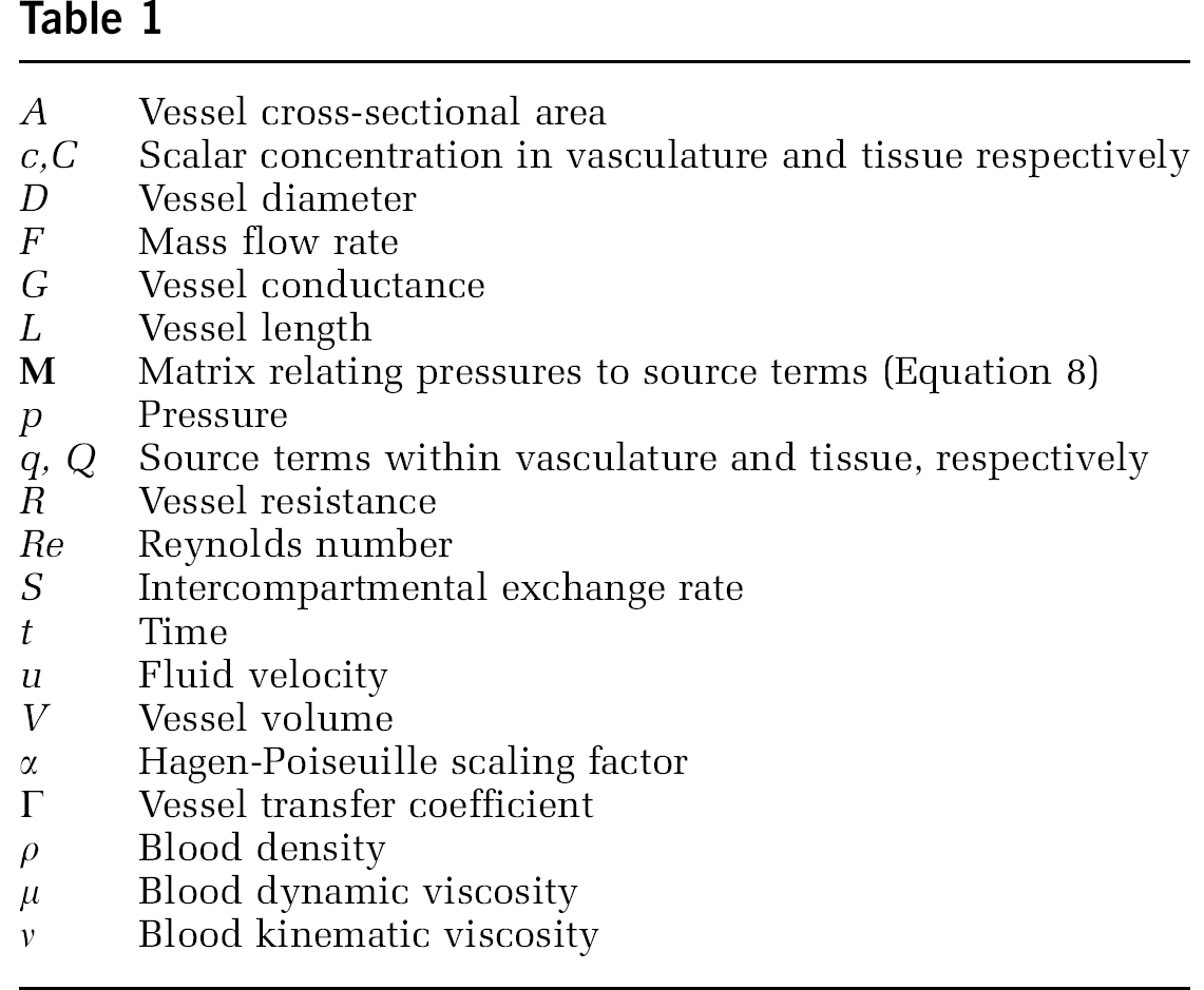
Table of Variables

The following table gives an overview of all variables that are used throughout the paper. Within the text or formulae, individual parameters may have additional superscripts or subscripts as well as overbars. Single subscripts denote node indices of node-based quantities. Double subscripts signify edge-centered parameters (e.g., L_ij is the length of the edge connecting nodes i and j). Superscripts and overbars denote iteration levels and upscaled quantities, respectively.

Table 1

A	Vessel cross-sectional area
c, C	Scalar concentration in vasculature and tissue respectively
D	Vessel diameter
F	Mass flow rate
G	Vessel conductance
L	Vessel length
M	Matrix relating pressures to source terms (Equation 8)
P	Pressure
q, Q	Source terms within vasculature and tissue, respectively
R	Vessel resistance
Re	Reynolds number
S	Intercompartmental exchange rate
t	Time
u	Fluid velocity
V	Vessel volume
a	Hagen-Poiseuille scaling factor
T	Vessel transfer coefficient
P	Blood density
μ	Blood dynamic viscosity
V	Blood kinematic viscosity

Implementation of the Vascular Graph Framework

We have implemented the VG modeling framework described above with a custom C ++ code. It comprises an input routine that can read Amira file-formats (see subsection ‘Vascular network generation from srXTM images’) to produce its own representation of the VG. The code further offers the possibility to set pressure boundary conditions at specific nodes, as well as to manually change properties of individual vessels, such as their diameter before solving for pressure and blood flow.

Results

Blood Pressure and Cerebral Blood Flow

Following the procedure outlined in the methods section, the pressure and flow fields were computed for the test domain (see Supplementary Figure for an example).

We find that pressure drops are comparatively small in the large feeding and draining vessels and most pronounced in the precapillary arterioles. In our simulations, the mean arterial blood flow velocity exceeds that of the veins by a factor of 1.99. This is a direct result of the fact that the total cross-sectional area of the arteries is lower than that of the veins, despite their higher abundance.

The total flow entering the gray matter region of the sample amounts to 1.80e-11 m³ s⁻¹. With a domain volume of 2.8 mm³, of which the gray matter occupies around 65%, this scales to a CBF of 59.3 mL min⁻¹ 100 mL⁻¹, which compares well with the in vivo values measured by Weber et al (2003).

Effect of Local Vascular Change

Arteriolar vessels were dilated by 10% to mimic local vascular changes that occur during functional hyperemia. Three different scenarios were considered: a feeding artery that spans the gray matter region in its entirety was dilated once just upstream of the capillary bed, and once a short distance downstream of the pial vessels. The third case is the dilation of an artery that supplies only the superior cortical layers.

As expected, the results show that arteriolar dilation leads to an increase in flow in the feeding vessel, as well as the connected capillary network and draining veins downstream of the dilation site. The core of the response is a blood flow increase of 10.3%, 2.8%, and 1.5%, respectively (cases 1 to 3 in Figure 3). The simulation further suggests that the flow increase in the capillary bed is predominantly restricted to a maximal cortical depth that coincides with the depth at which the feeding arteriole has its most inferior collaterals.

Figure 3

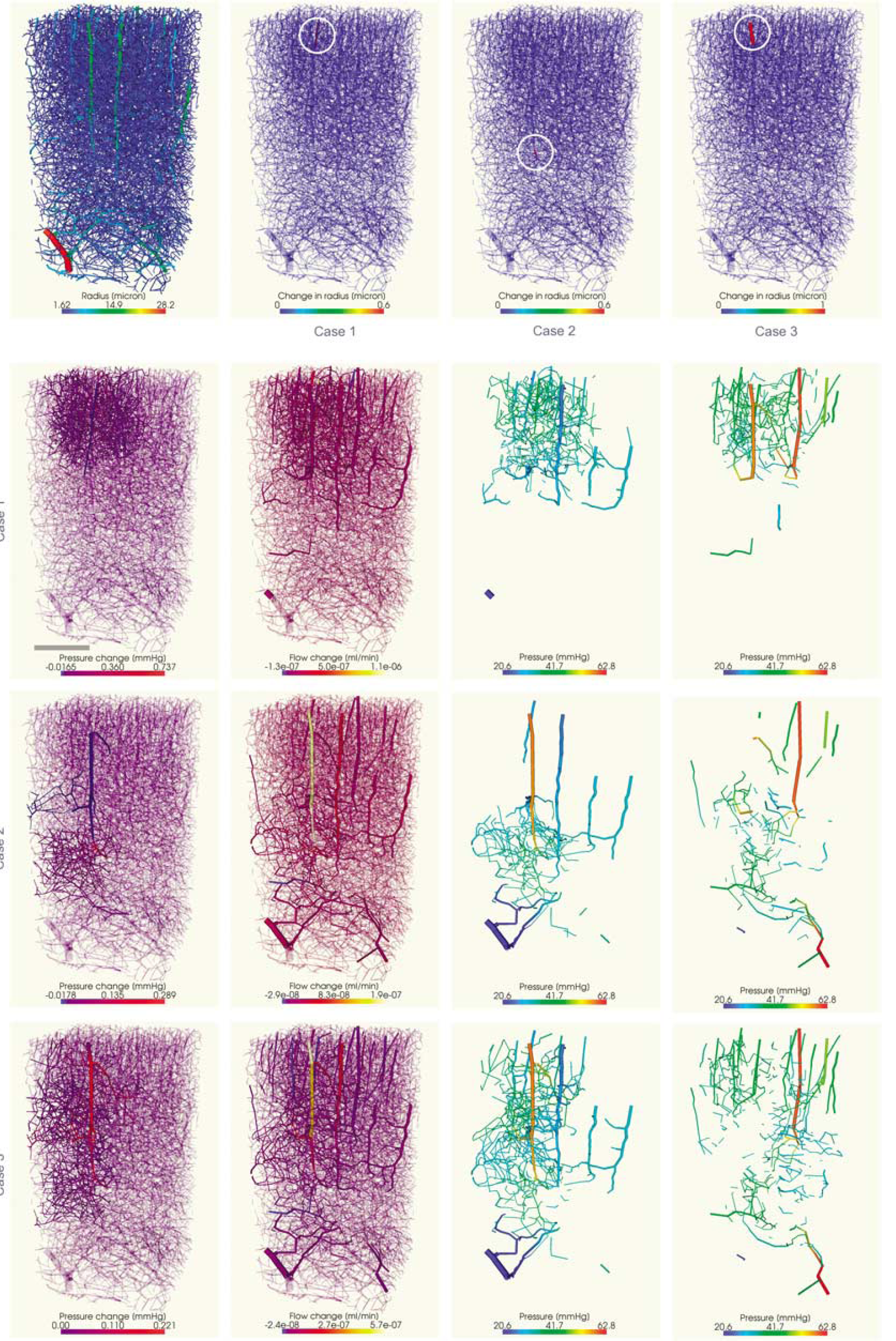
Dilation of different feeding arteries and/or at different cortical depths. Scale bar, 500 μm. The top row shows the vascular network color coded by radius (leftmost) as well as the individual sites of dilation highlighted by white circles: short feeding artery dilated near the cortical surface, long artery dilated just upstream of the capillary bed, long artery dilated near the cortical surface (row 1, columns 2 to 4, respectively). Rows 2 to 4 depict the respective change in pressure (first column) and flow (second column) resulting from the dilations. Major changes have been highlighted. Columns 3 to 4 show vessels where flow increases/decreases respectively, colored with pressure values to facilitate artery/vein distinction.

Other feeders in the vicinity and their respective connecting capillaries experience a decrease in flow. This decrease, however, is less pronounced than the corresponding flow increase.

Rows 3 to 4 in Figure 3 show that the spatial specificity of flow alterations depends strongly on the position of the local diameter change in the vascular hierarchy. The closer to the cortical surface the dilation occurs, the larger is its region of influence. However, a diameter increase just before the capillary bed may locally lead to stronger flow increase than one further upstream.

An occlusion scenario was created by constricting the diameter of a feeding artery to 1/1000 of its original size (Figure 4).

Figure 4

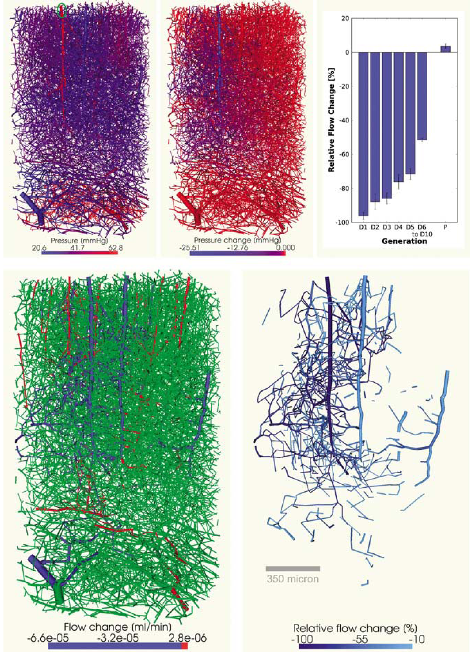
Occlusion of a penetrating cortical arteriole. Top row, left: initial vascular network color-coded by pressure. A green ellipse indicates the site of the occlusion. Top row, middle: change in pressure due to the occlusion. Top row, right: blood flow change categorized by topology. D1 denotes the first generation of vessels that branch off the penetrating arteriole, D2 denotes vessels that branch off the D1 generation and so on. Penetrating arterioles parallel to the occluded arteriole fall under category R The error bars indicate the standard error of the mean. Bottom row: Absolute change in flow, relative change in flow within the interval [-10%, −100%].

The simulation indicates that the occlusion of an arteriole has a marked effect on the blood flow in the capillary bed it irrigates, as well as the veins that it is most strongly linked to. By performing a breadth first search of the VG, starting at nodes that belong to the occluded arteriole, we have acquired a quantitative measure of flow change based on vessel topology. We find that blood flow slowly recovers towards baseline with increasing numbers of bifurcations away from the occluded penetrating arteriole as the influence of adjacent feeding arterioles increases. However, at 6 to 10 bifurcations away from the occluded vessel, flow values are still lower than half baseline. Moreover, a flow increase in the surrounding arterioles of around 3.6% can be observed. This change, however, cannot compensate the severe drop in CBF in those regions that were irrigated by the occluded arteriole.

It should be noted that both Figure 3 and Figure 4 show the VG representation of the vasculature. Vertices are not represented graphically, while edges are depicted by straight cylinders, whose diameter equals the mean diameter of the original tortuous vessels. The connectivity of the VG can be expected to be lower than true connectivity, due to small imperfections that may arise in sample preparation, data acquisition, and postprocessing.

Upscaling of the Capillary Bed

An artificial (unphysiological) two-dimensional network was constructed. It consists of capillaries with a diameter of 1 [arbitrary units] and noncapillaries whose diameter is up to 10 times larger, arranged in a quarter five-spot configuration (Figure 5, top left). High-pressure/low-pressure boundary conditions were set at the noncapillary corner nodes/central node, respectively. Within two circular regions, the capillary diameter was increased by 10%. The fluid flow was computed both before and after this network modification. The resulting change in flow is shown qualitatively in the top right of Figure 5. The flow increases in three of the four noncapillary vessels, in those areas in which the capillaries have been dilated, and in the directions that connect them to the nearest noncapillary vessels. Perpendicular to the direction of flow increase, the flow decreases.

Figure 5

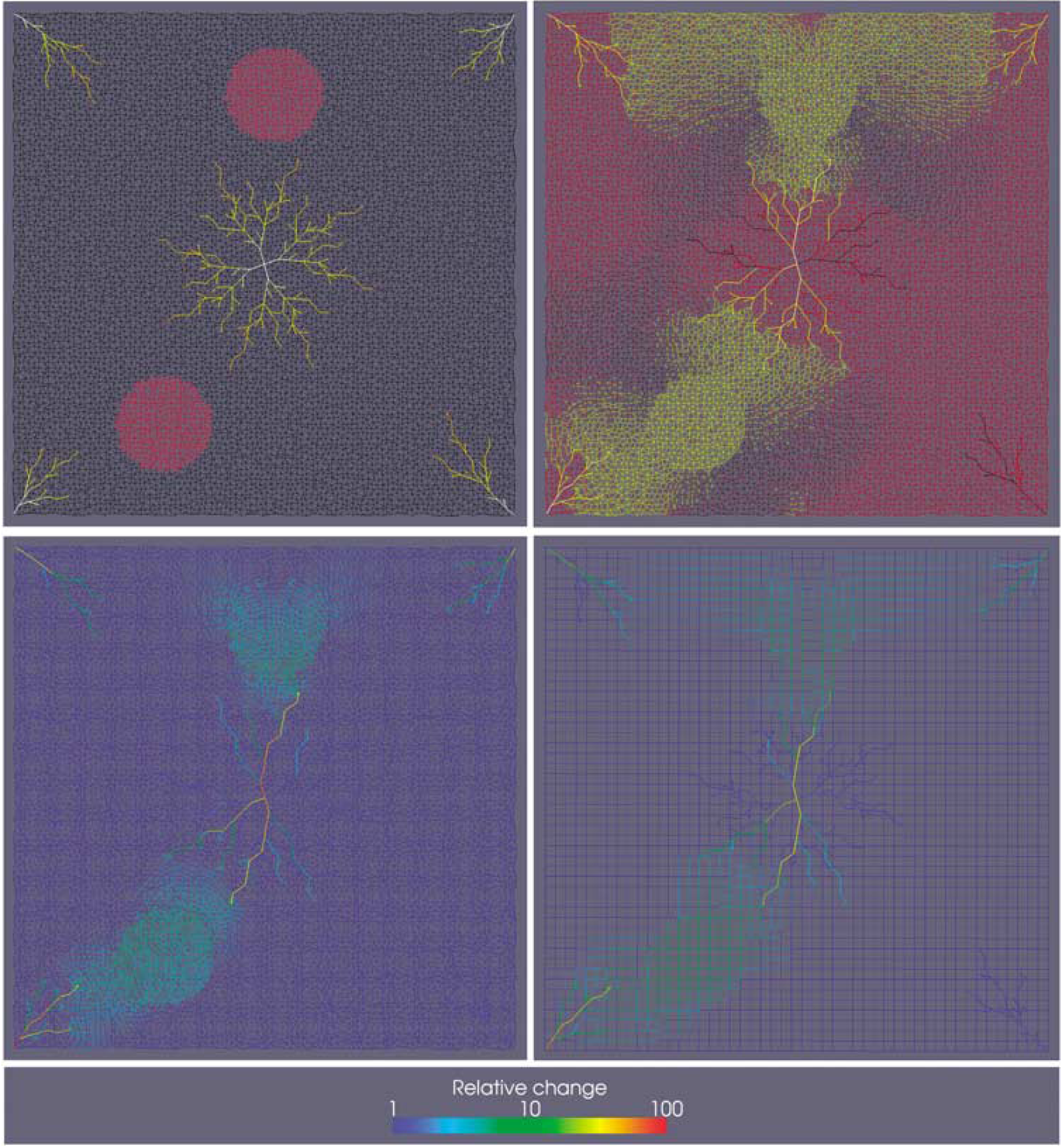
Artificial two-dimensional vascular network consisting of two vessel types (capillaries and noncapillaries). The noncapillaries are arranged in a quarter five-spot configuration, i.e., one complete vascular tree in the center of the domain, and a quarter tree at each of the four corners. Top left: The noncapillary vessels at the center and the corners have a maximum diameter of 10 [arbitrary units]. The diameter decreases linearly with distance from the center/corner, respectively. Low/high-pressure boundary conditions are set at the center-node/corner-nodes, respectively. The black mesh depicts the capillary network with vessel diameters of 1. At two circular regions, the capillary diameter has been increased by 10% (shown in red). Top right: Thresholded image of the changes in flow that result from the capillary dilation. Vessels colored in yellow experience an increase in flow, whereas black vessels denote a flow decrease. Vessels colored in red are not subject to flow change. Bottom row: Change in fluid flow due to the dilations in the capillary network. Values are scaled relative to the maximum change in the domain. Left: flow in the fully resolved vascular network with > 10 000 nodes. Right: flow in the upscaled network, consisting of <3000 nodes.

In total, the network consists of > 10,000 vertices. Using the methodology described above, the discrete capillary network was upscaled, reducing the number of nodes to < 3000, and the flow simulations were repeated. The bottom row of Figure 5 depicts how the upscaled representation compares with the discrete case.

There is good qualitative and quantitative agreement between the two cases as both the flow topology and values are captured well by the upscaled network. The absolute flow values through the four corner nodes and the central node of the noncapillary vessels differ by <10%. In this simple two-dimensional setup, the number of nodes has been reduced by a factor of approximately two in each coordinate direction. This coarsening factor might be much larger in other situations and particularly in three-dimensional the number of degrees of freedom can be dramatically reduced.

Scalar Transport and Diffusion

The two-dimensional testcase above was extended to include a simple tissue representation in the form of a homogeneous structured network. As initial and boundary condition, the concentration of the scalar in the tissue graph was set to one at those locations that coincide with the dilated capillary regions (see Figure 5, top left). In the VG, the scalar concentration was initially set to zero. Exchange of scalar between tissue and vasculature was enabled for the capillary network. Figure 6 shows the evolution of the scalar distribution at several time points.

Figure 6

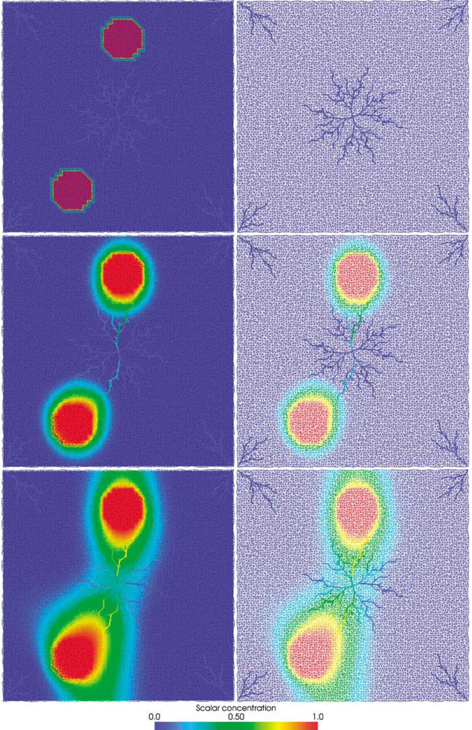
Diffusion and transport of an arbitrary scalar. The plots in the left column show an overlay of the tissue and vascular graph. The discrete vascular graph has been interpolated to emphasize that it is an approximation of a continuum. The right column depicts the vascular graph on its own (vessel thickness has been increased for better visibility). Top row: Initially, the scalar concentration is set to one in two circular regions of the tissue and to zero everywhere else, including the entire vasculature. The tissue nodes within these circular regions are set as sources that produce a constant scalar inflow throughout the simulation. Middle row: Distribution of the scalar after 100 time steps. The scalar has diffused within the tissue and some exchange with the vasculature has occurred. Within the vasculature, the scalar is transported towards the central low-pressure node. Bottom row: Steady state scalar concentration. Compared with a scenario with homogenous diffusion in tissue, the scalar distribution is elongated in the direction of the vascular flow.

The scalar propagates throughout the tissue by means of diffusion. Owing to the concentration gradient, a fraction of it is taken up by the vascular compartment. Here, the scalar is advected towards the low-pressure node in the center of the domain. Because of the constant inflow and outflow, after a transitional phase, eventually a steady state is reached. The exchange between tissue and vasculature results in a distribution that is elongated along the direction of the vascular flow. The local scalar concentrations in both compartments match due to the concentration gradient based exchange, except for the circular regions in which the tissue concentration is fixed.

Discussion

In this paper, we present a modeling framework for CBF in realistic vascular networks. It operates on vascular anatomical data of any kind, as long as the vessel conductance can be extracted.

We have proposed an upscaling algorithm that facilitates the application of the VG model to large vascular networks by a combination of complexity reduction and flow-characteristics preservation. Furthermore, it extends the model's applicability to scenarios in which the discrete topology of the capillary bed is unknown, but coarse-scale conductance information is available.

The transport of arbitrary scalar quantities within the vascular network can be simulated, with an exchange term describing the transfer between vasculature and tissue. Finally, the VG model also incorporates the diffusion of the scalar within the tissue.

A major strength of the VG model is the fact that vascular properties such as vessel length, diameter, and elasticity can be manipulated easily.

The effect of local arteriolar dilation on CBF can be simulated by manually increasing the diameter of a specific vessel, recomputing the CBF and comparing the results with the basal state. Similarly, cerebrovascular pathologies can be studied by reducing diameters (occlusion scenarios), decreasing elasticity values or alike. Naturally, vascular changes may not occur as isolated as described here. Arteriolar dilation, for example, might be accompanied by simultaneous constriction of the feeding vessels in the vicinity. The model currently does not include this active surround regulation automatically, because our understanding of these effects is still limited. However, the VG framework certainly supports this kind of behavior, it merely needs to be prescribed manually. Therefore, a close interplay between simulation and experiment is the key to further our understanding of the CBF and its regulation.

Simulation Results

The pressure distributions computed in our simulations are in good agreement with literature as they show the steepest pressure drop at the arteriolar level. Thus, the arterioles present the highest resistance to flow and consequently are ideal locations for flow regulation by way of smooth muscle relaxation/constriction.

The blood flow computations yield gray matter CBF of about 60 mL min⁻¹100 mL⁻¹, which compares well with our in vivo measurements (Weber et al, 2003). Nevertheless, flow values published elsewhere (Nakao et al, 2001; Wegener et al, 2007), suggest that our simulation slightly underestimates CBF. Partly, this may stem from the imperfect connectivity of the vasculature in our samples. Incomplete filling with BaSO₄ during the perfusion process as well as image processing algorithms may lead to interrupts in the reconstructed sample that increase the net resistance to blood flow. Moreover, the part of the sample's vasculature that is connected to feeding arterioles outside the domain lacks irrigation, further adding to a possible underestimation of CBF.

Our simulations reproduce the well-known fact that arteriolar dilation leads to a flow increase in the feeding vessel, as well as the connected capillary network and draining veins further downstream. The computations suggest that there exists a spatial specificity that is prescribed by the topology, i.e., the type of feeding artery (Duvernoy et al, 1981). That is, the cortical depth at which the artery has its most inferior collaterals often determines the maximal depth of the major flow increase in the capillary bed. This confirms our finding that the structure of the capillary bed is not isotropic, but rather is optimized for mass transport predominantly parallel to the cortical surface (manuscript in preparation). The spatial specificity of dilation-induced CBF changes further depends on the dilated vessel's position in vascular hierarchy. The closer the alteration is to the cortical surface, the larger its region of influence. However, the local magnitude of the resulting flow-change also depends on the distance to the dilation site.

As an artery or arteriole dilates, its resistance to flow decreases, leading to flow redistributions in the system of parallel arterioles which it is a part of. Feeding arteries in the vicinity of the dilation site experience a decrease in flow, an effect that has been described earlier (Boas et al, 2008 and citations therein). Our simulations capture this phenomenon and the absolute flow values show that the decrease is small compared with the flow increase in the dilated arteriole.

Individual vessel-diameters of feeding arteries were reduced to create occlusion scenarios. Our simulations indicate that the CBF decrease is most strongly expressed in the capillary bed formerly irrigated by the occluded arteriole and the adjoining draining veins. The relative flow decrease just downstream of a total occlusion is 100%, but flow values recover with increasing number of bifurcations until eventually the influence of the occlusion is negligible.

Nishimura and coworkers have used focal photo-thrombosis to occlude single penetrating arteries in vivo (Nishimura et al, 2007). Their results indicate that these vessels are the bottleneck in neocortex-perfusion and show that the region of influence of an occluded penetrating arteriole is 350 μm, consistent with that vessel type's spatial distribution. Our occlusion simulations yield regions of influence that are in accordance with the experimental findings. Moreover, also the topological characteristics of experiment data and simulations compare favorably. Within the first five generations of vessels that branch off the occluded penetrating arteriole, the fractional change in blood flow recovers from −1.0 to −0.7 approximately. In addition, our simulations show that occlusions may also lead to an increase in flow in unblocked arterioles located in the vicinity of the occlusion. (The data of Nishimura and coworkers also suggest this, but due to a comparably high standard error of the mean, this finding is not statistically significant.) Blood pressure drops in the capillaries downstream of an occlusion, thus increasing the pressure difference between other (nonoccluded) feeding arterioles and this region of the capillary bed. However, as the largest pressure drop occurs at arteriolar level, the increase in pressure difference, and consequently in blood flow, is not as pronounced. We find that the largest decrease in flow is > 20 times stronger than the largest increase (absolute flow values). That is, the increase in flow in the neighboring arterioles cannot compensate the severe drop in CBF due to the occlusion.

Comparison With Earlier Work

The underlying principles of the proposed modeling framework are in many respects similar to those introduced by Boas and coworkers in their compelling vascular anatomic network model: the cerebral vasculature is represented by a network of cylinders/vessels, each of which has a resistance to flow according to the Hagen-Poiseuille law. The flow of blood is driven by pressure differences across the vessels. Pressure boundary conditions are set at the feeding arteries and draining veins, for which literature values exist (Zweifach 1974). Boas' vascular anatomic network model and our VG model both are an extension to the serial pipe model in that branching nodes are introduced at which flow is conserved.

Buxton and coworkers introduced the idea of a compliant venous compartment in their balloon model (Buxton et al, 1998). It relates the temporal changes in CBV to the blood oxygenation level dependent effect and offers an explanation for the mismatch between the time courses of blood flow and blood volume. Mandeville et al have extended this idea with the Windkessel model (Mandeville et al, 1999), which specifies the physiological parameters of the flow-volume relationship. Specifically, the model links changes in pressure to diameter changes. This relation is used both in Boas' and our simulations.

While the focus of Boas and coworkers lies on the reduction of complexity to create a simple, yet representative vascular network, we show that the modeling framework is applicable to realistic angioarchitecture. A major extension to the vascular anatomic network model in this respect is the transition to fully three-dimensional tissue-vasculature interactions. We have introduced a three-dimensional tissue representation that designates the tissue continuum in which the vasculature is embedded. This allows modeling the transport of scalar quantities within the tissue by way of diffusion as well as a more realistic exchange between vasculature and tissue as one tissue volume can be linked to multiple blood vessels and vice versa. The tissue source term can be specified locally (e.g., local CMRO2 can be prescribed when modeling oxygen transport) and influences the exchange between vasculature and tissue according to their relative positions in three-dimensional space. Recently, Fang and coworkers have proposed a similar approach (Fang et al, 2008), in which a tetrahedral mesh discretizes the vascular compartment.

Finally, we have introduced an upscaling approach to replace the discrete representation of the capillary bed. While retaining a high degree of accuracy, the computational cost is dramatically reduced, which is important when studying dynamic effects (or other scenarios that require frequent recomputation) in large vascular networks. The upscaling algorithm further allows treating scenarios for which no detailed topological information of the vasculature is available as long as coarser-scale statistical information on the system is accessible.

Outlook

A major challenge when working with angiography data is setting appropriate boundary conditions. Currently, we are relying on literature (Zweifach, 1974) to determine pressure boundary conditions for large feeding arteries and draining veins. As systemic blood pressure does not vary much in between species, we expect only minor errors when applying Zweifach's data of cat models to our rat srXTM samples. Nevertheless, we are currently working on obtaining accurate in vivo pressure values for the rat vasculature.

Vessels at the border of the srXTM samples often have unphysiological dead ends as they connect to vasculature beyond the domain of the sample. Consequently, we have set no-flow boundary conditions at these end points, as accurate pressure values are not available. This implies that all blood that enters through the sample's feeding arteries must exit through its draining veins. In reality, however, the drainage would also involve veins outside of the sample. Therefore, the changes in blood flow due to dilations or constrictions are artificially confined to the size of the domain.

Another issue concerns the approach used to differentiate arteries from veins in the srXTM data. We are currently refining our imaging and vessel identification methods, to further reduce the uncertainties in this respect.

Upcoming projects aim to harness the srXTM sample-database to produce lookup tables of vessel diameter, length, and angular distribution. These tables in turn will be used to generate realistic artificial vascular networks. The artificial networks have the dual advantage of perfect connectivity and no size limitations. This helps to circumvent the problem regarding boundary conditions discussed above. The effect under investigation can be placed as far away from the sample's boundaries as needed to nullify the influence of the (possibly incorrect) boundary conditions.

Several studies have shown that erythrocyte transport at bifurcations depends on the diameters of the daughter vessels (Fenton et al, 1985; Pries et al, 1989; Yan et al, 1991). Future versions of the VG model will aim to incorporate this knowledge to compute accurate hematocrit and relative apparent viscosity values for any given topology.

As Boas et al have pointed out, the framework may be extended to include arterial compliance, which has been reported recently (Behzadi and Liu, 2005).

Finally, work is in preparation to generate srXTM data from the macaque monkey cortex and compare simulation results with those performed using rat vasculature.

In conclusion, we have proposed a framework that models the flow of blood through the cerebral vasculature, based on simple fluid dynamics principles. It includes fully three-dimensional advective transport, vasculature-tissue exchange and diffusion within the tissue, allowing to simulate oxygen transport, drug delivery and alike. Upscaling algorithms facilitate its application to large-scale networks and dynamic systems. The VG framework provides a means to investigate the flow properties of case (patient) specific vascular networks. Moreover, it can be used as a powerful tool to research the effects of vascular changes on the CBF.

Footnotes

Acknowledgements

We thank Dr Federica Marone, Swiss Light Source, Paul Scherrer Institut, Villigen, Switzerland, for her kind assistance at the synchrotron beamline and Dr Bernhard Stalder, Bühler AG, Uzwil, Switzerland, for his invaluable help with the barium sulfate dispersion.

The authors declare no conflict of interest.

Notes

Supplementary Information accompanies the paper on the Journal of Cerebral Blood Flow & Metabolism website ()

References

Behzadi

Liu

(2005) An arteriolar compliance model of the cerebral blood flow response to neural stimulus. Neuroimage 25:1100–11

Boas

Jones

Devor

Huppert

Dale

(2008) A vascular anatomical network model of the spatio-temporal response to brain activation. Neuroimage 40:1116–29

Buxton

Wong

Frank

(1998) Dynamics of blood flow and oxygenation changes during brain activation: the balloon model. Magn Reson Med 39:855–64

Castro

Putman

Cebral

(2006) Patient-specific computational modeling of cerebral aneurysms with multiple avenues of flow from 3d rotational angiography images. Academic Radiol 13:811–21

Duvernoy

Delon

Vannson

(1981) Cortical blood vessels of the human brain. Brain Res Bull 7:519–79

Fang

Sakadzic

Ruvinskaya

Devor

Dale

Boas

(2008) Oxygen advection and diffusion in a three-dimensional vascular anatomical network. Optics Express 16:17530–41

Fenton

Carr

Cokelet

(1985) Nonuniform red cell distribution in 20 to 100 micrometers bifurcations. Microvasc Res 29:103–26

Kwong

Belliveau

Chesler

Goldberg

Weisskoff

Poncelet

Kennedy

Hoppel

Cohen

Turner

(1992) Dynamic magnetic resonance imaging of human brain activity during primary sensory stimulation. Proc Natl Acad Sci USA 89:5675–9

Lipowsky

Zweifach

(1974) Network analysis of microcirculation of cat mesentery. Microvasc Res 7:73–83

10.

Lipowsky

Usami

Chien

Pittman

(1980) Hematocrit determination in small bowel bore tubes from optical density measurements under white light illumination. Microvasc Res 20:51–70

11.

Mandeville

Marota

Ayata

Zaharchuk

Moskowitz

Rosen

Weisskoff

(1999) Evidence of a cerebrovascular postarteriole Windkessel with delayed compliance. J Cereb Blood Flow Metab 19:679–89

12.

Mosso

(1881) Ueber den Kreislauf des Blutes im Menschlichen Gehirn. Leipzig: Von Veit

13.

Nakao

Itoh

Kuang

Cook

Jehle

Sokoloff

(2001) Effects of anesthesia on functional activation of cerebral blood flow and metabolism. Proc Natl Acad Sci USA 98:7593–8

14.

Nishimura

Schaffer

Friedman

Lyden

Kleinfeld

(2007) Penetrating arterioles are a bottleneck in the perfusion of neocortex. Proc Natl Acad Sci USA 104:365–70

15.

Ogawa

Lee

Kay

Tank

(1990) Brain magnetic resonance imaging with contrast dependent on blood oxygenation. Proc Natl Acad Sci USA 87:9868–72

16.

Parkes

Tofts

(2002) Improved accuracy of human cerebral blood perfusion measurements using arterial spin labeling: accounting for capillary water permeability. Magn Reson Med 48:27–41

17.

Plouraboue

Cloetens

Fonta

Steyer

Lauwers

Marc-Vergnes

(2004) X-ray high-resolution vascular network imaging. J Microsc 215:139–48

18.

Pries

Ley

Claassen

Gaehtgens

(1989) Red cell distribution at microvascular bifurcations. Microvasc Res 38:81–101

19.

Pries

Neuhaus

Gaehtgens

(1992) Blood viscosity in tube flow: dependence on diameter and hematocrit. Am J Physiol 263:H1770–8

20.

Roy

Sherrington

(1890) On the regulation of the blood supply of the brain. J Physiol 11:85–108

21.

Schaffer

Friedman

Nishimura

Schroeder

Tsai

Ebner

Lyden

Kleinfeld

(2006) Two-photon imaging of cortical surface microvessels reveals a robust redistribution in blood flow after vascular occlusion. PLoS Biol 4:e22

22.

Tsoukias

Goldman

Vadapalli

Pittman

Popel (2007) A computational model of oxygen delivery by hemoglobin-based oxygen carriers in three-dimensional microvascular networks. J Theor Biol 248:657–74

23.

Turner

(2002) How much cortex can a vein drain? Downstream dilution of activation-related cerebral blood oxygenation changes. Neuroimage 16:1062–7

24.

Weber

Späth

Wyss

Wild

Burger

Stanley

Buck

(2003) Quantitative cerebral blood flow measurements in the rat using a beta-probe and H2 150. J Cereb Blood Flow Metab 23:1455–60

25.

Weber

Keller

Reichold

Logothetis

(2008) The microvascular system of the striate and extrastriate visual cortex of the macaque. Cerebral Cortex 18:2318–30

26.

Wegener

Perthen

Wong

(2007) Quantification of rodent cerebral blood flow (CBF) in normaland high flow states using pulsed arterial spin labeling magnetic resonance imaging. J Magn Reson Imaging 26:855–62

27.

Weinberg

(1962) Network Analysis and Synthesis. New York: McGraw-Hill

28.

Yan

Acrivos

Weinbaum

(1991) A three-dimensional analysis of plasma skimming at microvascular bifurcations. Microvasc Res 42:17–38

29.

Zhou

Wilson

Ulatowski

Traystman

van Zijl

(2001) Two-compartment exchange model for perfusion quantification using arterial spin tagging. J Cereb Blood Flow Metab 21:440–55

30.

Zweifach

(1974) Quantitative studies of microcirculatory structure and function. I. Analysis of pressure distribution in the terminal vascular bed in cat mesentery. Circ Res 34:843–57

Supplementary Material

Please find the following supplemental material available below.

For Open Access articles published under a Creative Commons License, all supplemental material carries the same license as the article it is associated with.

For non-Open Access articles published, all supplemental material carries a non-exclusive license, and permission requests for re-use of supplemental material or any part of supplemental material shall be sent directly to the copyright owner as specified in the copyright notice associated with the article.

0.00 MB

0.19 MB

Vascular Graph Model to Simulate the Cerebral Blood Flow in Realistic Vascular Networks

Abstract

Keywords

Introduction

Materials and methods

Basic Model Concepts

Model Network Construction

Synchrotron Radiation Based X-Ray Tomographic Microscopy (srXTM) of Brain Vasculature

Vascular Network Generation from srXTM Images

Classification of Large Vessels

Governing Equations

Computation of Pressure and Mass Flow

Elasticity

Upscaling of the Fine-Scale Vascular Structures

Scalar Transport

Table of Variables

Implementation of the Vascular Graph Framework

Results

Blood Pressure and Cerebral Blood Flow

Effect of Local Vascular Change

Upscaling of the Capillary Bed

Scalar Transport and Diffusion

Discussion

Simulation Results

Comparison With Earlier Work

Outlook

Footnotes

Acknowledgements

Notes

References

Supplementary Material