Sage Journals: Discover world-class research

Abstract

We have designed and fabricated a polydimethylsiloxane (PDMS) microfluidic device for coupling capillary electrophoresis (CE) and matrix-assisted laser desorption ionization-mass spectrometry (MALDI-MS). The coupling is advantageous in biological research because CE has the power of separating analytes in a sample based on mobility difference and MALDI-MS provides accurate and sensitive mass analysis of the analytes. The goal is realized by fractionating the separated analytes inside the microfluidic device and pushing the analyte fractions into open reservoirs. Each analyte fraction is then mixed with a matrix solution and deposited on a MALDI target for MALDI-MS. Therefore, a two-step analysis of analytes in the form of CE-MALDI-MS is achieved by using the microfluidic device.

Keywords

capillary electrophoresis MALDI–MS microfluidic device

Introduction

Recent developments of mass spectrometry (MS) have substantially expanded its application to the biological research fields.^{1

–5} In particular, the soft ionization methods, including electrospray ionization (ESI) and matrix-assisted laser desorption ionization (MALDI), have made MS a powerful analytical tool for biological samples. To exploit the larger power, ESI-MS and MALDI-MS are often coupled with chromatography, such as high-performance liquid chromatography (HPLC) and capillary electrophoresis (CE), resulting in a two-step analysis of analytes in a sample. The chromatography provides the power of separating analytes, which significantly broadens the application of ESI-MS and MALDI-MS to samples with complicated composition.^{6

–10} A number of techniques have been reported for coupling these powerful technologies, such as coupling HPLC and ESI-MS,^11,12 CE and ESI-MS,^13,14 HPLC and MALDI-MS,^{15

–19} and CE and MALDI-MS.^{20

–24} In addition to these examples, a particular case is coupling gel isoelectric focusing (IEF) and MALDI-MS, which is a modification of the widely used two-dimensional (2D) electrophoresis and often named as virtual 2D electrophoresis.²⁵ To achieve the two-step analysis of samples at a small volume, microfluidic devices are often used as the platforms for coupling chromatography and MS.^{26
–28}

Compared with other methods, coupling CE and MALDI-MS is not reported as often. A reason for this is the difficulty in establishing the interface between CE and MALDI-MS. Usually for the purpose of connecting chromatography to MALDI-MS, the eluted analytes are fractionated and deposited on a MALDI target to prepare MALDI sample spots. However, in CE the motion of analytes is driven by an electric field applied in the capillary, which makes it difficult to directly deposit eluted analytes to a MALDI target.^20,21 Murray and coworkers proposed a strategy of using a rotating ball interface in a silicon microfluidic device.²² The specially constructed rotating ball serves as both the electrode for CE and the inlet carrying the eluted analytes to MALDI-MS. However, this strategy requires substantial efforts to fabricate and precisely manipulate the microfluidic device. An alternative strategy was reported to carry out CE separation in an open channel, where the separated analytes were directly ionized from the open channel to a mass spectrometer.^23,24 However, gel was filled into the open channel to suppress electroosmotic flow (EOF) and reduce analyte dispersion after the CE separation. This strategy is applicable to capillary gel electrophoresis but not to regular free-solution CE modes.

A straightforward strategy for coupling CE and MALDI-MS is using pressure-driven flow to elute analytes to a MALDI target after the CE separation is finished. However, due to analyte dispersion, re-mixing of separated analytes may happen during the elution. To prevent re-mixing of the separated analytes, fractionation of separated analytes is needed between the CE separation and the elution. For the purpose of fractionating analytes immediately after the CE separation, we have designed and fabricated a polydimethylsiloxane (PDMS) microfluidic device. It realizes CE separation of analytes in a sample followed by in-place fractionation of the separated analytes. The microfluidic device also facilitates easy transfer of the analyte fractions to a MALDI target. The manipulation in the microfluidic device is carried out in three steps: (1) the analytes are loaded and separated in a CE channel; (2) the separated analytes are fractionated in the CE channel; and (3) the analyte fractions are transported into the fraction reservoirs by pressure-driven flow. Then some external tool is used to transfer the analytes out of the microfluidic device for MALDI-MS. The manipulation in the microfluidic device is facilitated by built-in actuators, such as valves and pumps. The elasticity of PDMS simplifies the construction of these actuators in the microfluidic device, in contrast to those made of rigid materials. The microfluidic device performs as a platform for coupling CE and MALDI-MS, resulting in a two-step analysis of a sample.

Experimental

Chemicals and Reagents

Neurotensin (NRT), [Glu1]-Fibrinopeptide B (FPB) and Lys-[Des-Arg9]-Bradykinin (BRK) were purchased from American Peptide Company (Sunnyvale, CA). Platelet-Derived Growth Factor Receptor Substrate 1 (PS1) was purchased from Anaspec (San Jose, CA). Peptide NYISKGSTFL, the dephosphorylated form of PS1 (DP-PS1) was synthesized by Elim Biopharmaceuticals (Hayward, CA). MALDI matrices α-cyano-hydroxycinnamic acid (CHCA) and 2,5-dihydroxybenzoic acid (DHB), methyltrichlorosilane (MTS) and 10% sodium dodecylsulfate (SDS) solution were purchased from Sigma–Aldrich (St Louis, MO). Dodecyl-β-d-maltoside (DDM) was obtained from Anatrace (Maumee, OH). Fluorescent reagents Cy5 NHS ester (Cy5) and Alexa Fluor 647 carboxylic acid succinimidyl ester (AR647) were purchased from Invitrogen (Carlsbad, CA) and GE (Fairfield, CT), respectively. PDMS prepolymer RTV 615A and 615B were obtained from GE (Fairfield, CT). Photolithography reagents were provided by Stanford Nanofabrication Facility (Stanford, CA).

Design and Fabrication of the Microfluidic Device

Figure 1A shows the layout of the microfluidic device, which is composed of two layers. The lower layer, called the flow layer, is used for manipulation of analytes, including CE separation, fractionation, and fraction transport. It contains a sample loading channel, a CE channel and a set of branch channels (orange), and each channel has a width of 150 μm and a height of ∼15 μm. All channels are connected to reservoirs for introducing reagents into the channels. The leftmost and rightmost reservoirs are electrolyte reservoirs, where electrodes are placed to apply a voltage during CE separation. The sample-loading channel is perpendicular to the CE channel, and the intersection is where analytes are loaded in the CE channel. For each branch channel, one end is connected to a small fraction reservoir and the other end is connected to a large shared reservoir that stores a channel-filling fluid. The shared reservoir is a rectangular channel loop with two circular reservoirs in the rectangular region, and the channel loop connects the channel-filling fluid from the circular reservoirs to all the fraction reservoirs. The fraction reservoirs have a diameter of ∼500 μm, whereas the other reservoirs and valve-openings have a diameter of ∼1.5 mm. The sample-loading channel is used to transport a sample into the CE channel. The set of branch channels form flow pathways for moving the analyte fractions into the fraction reservoirs. The upper layer, called the control layer, is used for control of the flow of analytes in the channels beneath, which is realized by actuators constructed in this layer. Three horizontal sets of valves (light green) form a monolithic peristaltic pump that actuates pressure-driven flow for fraction transport.²⁹ A row of vertical valves (dark green), called fractionation valves, are used to form compartments in the CE channel so that separated analytes can be fractionated in them. A horizontal valve (dark green), close to the fraction reservoirs is designed to prevent backflow from the fraction reservoirs when they are filled with the analyte fractions. A pair of horizontal valves (blue) on the left is used for making a sample plug in the CE channel and another pair of horizontal valves (blue) on the right for blocking the branch channels while CE is running. The valves and pumps are actuated by pressure conveyed through tubes connected to the valve-openings. The valves have a width of 200 μm or 300 μm (those in the pump) and a height of 55 μm. Figure 1B shows a picture of a fabricated microfluidic device.

Figure 1.

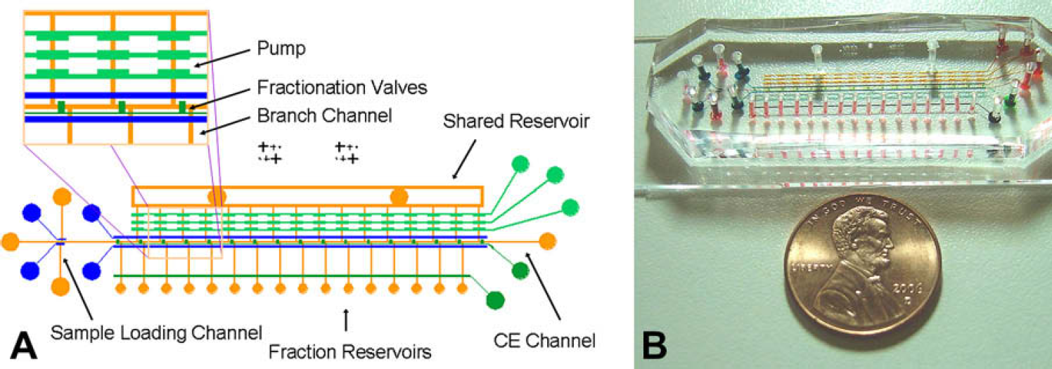
Microfluidic device designed for coupling CE and MALDI-MS. (A) Layout of the microfluidic device, in which a pump (light green) and valves (dark green and blue) in the control layer are aligned to the flow channels (orange) in the flow layer. The inset shows the enlarged structure around the CE channel. (B) Picture of a fabricated microfluidic device. For visualization, the pump, valves, channels, and reservoirs are filled with food coloring solution. A penny is used as a size marker.

The microfluidic device is fabricated by multilayer soft lithography. For fabricating PDMS layers, photoresist masters are formed on silicon wafers by photolithography to produce molds. The patterns of the photoresist masters are designed and printed on transparency films with high-resolution (40,640 dpi) to produce a mask. To make a mold for the flow layer, positive photoresist SPR 220–7 is spin-coated on a silicon wafer with a thickness of 10 μm and baked on a hotplate (95 °C for 200 s). The photoresist is exposed through the transparency mask and developed. The wafer is then baked in an oven (110 °C for at least 30 min) to reflow the photoresist so that round cross-sections are formed. To make a mold for the control layer, negative photoresist SU-8 is spin-coated on a silicon wafer with a thickness of 55 μm and baked twice (75 °C for 180 s and 105 °C for 360 s). The photoresist is exposed through the transparency mask, post-baked twice (75 °C for 60 s and 105 °C for 300 s) and developed. To prevent adhesion between PDMS and the molds, the molds are exposed to MTS vapor in a desiccator before use.

The control layer is made by pouring PDMS prepolymer (mixture of RTV A and B with a mass ratio of 10:1) on the mold to a thickness of ∼1 cm and curing PDMS in an oven (80 °C for 2 h). The control layer is peeled off the mold and holes are punched as openings. The flow layer is made by spin-coating (2.0 krpm for 60 s) PDMS prepolymer on the mold and curing the PDMS prepolymer in an oven (80 °C for 1 h). The control layer is aligned and attached to the flow layer. The attachment is carried out by a dipping–attaching method reported elsewhere.^30,31 Briefly, a solution of 1/10 (w/w) PDMS prepolymer in cyclohexane is spin-coated on a glass slide at 3.3 krpm to form a thin film. A PDMS layer is dipped into the thin film of PDMS prepolymer and attached to another PDMS layer. Thus between the two PDMS layers a portion of the thin film of PDMS prepolymer is present, which is then cured in an oven at 80 °C for 2 h to become an adhesive PDMS layer. To complete the microfluidic device, the two-layer PDMS block is attached to a PDMS-coated glass slide by the dipping–attaching method. Because of its low cost with batch fabrication, the microfluidic device is disposable after one-time use, thus saving the effort of device maintenance.

Running the Microfluidic Device

Figure 2 illustrates the steps of running the microfluidic device. For visualization, red food coloring solution is used instead of a real sample. In practice, all channels and reservoirs are first filled with the channel-filling fluid 0.05% DDM in water to wet the PDMS surfaces in the channels and reservoirs. The non-ionic surfactant DDM forms a dynamic coating on the PDMS surfaces to increase the hydrophilicity.³² Then the channel-filling fluid in the electrolyte reservoirs is replaced with the CE running buffer 20 mM ammonium bicarbonate at pH 8.5 with 0.05% DDM, 0.005% SDS, and 50 μg/mL BRK (average mass, 1032.2). By applying voltage in the electrolyte reservoirs, EOF is generated to fill the CE running buffer into the CE channel. The pH is adjusted with diluted ammonium hydroxide. The BRK in the CE running buffer serves as an internal standard for quantitation of analytes in MALDI-MS. To start the CE separation of analytes in a sample, the sample is added in one reservoir of the sample-loading channel and loaded in it by applying negative pressure in the other reservoir. By closing the valves on the sample-loading channel, a sample plug is formed in the CE channel. The CE separation is immediately started by applying a voltage along the CE channel. The CE separation is finished while the analytes are separated in the region between the outermost branch channels. At the same time, the fractionation valves are closed to form compartments in the CE channel, so that the separated analytes are fractionated into the compartments. Thus the volume of analyte fractions is at nanoliter-scale. The analyte fractions are transported into the fraction reservoirs by actuating the pump. The channel-filling fluid from the shared reservoir is used to push the analyte fractions into the fraction reservoirs as well as rinse the compartments and branch channels. The total volume of analyte solution accumulated in a fraction reservoir is controlled by the pumping rate and time. The total volume may be as low as the volume of a compartment plus a branch channel ∼18 nL. However, the analyte solution is usually ∼1 μL because an adequate amount is needed for transferring it out of the microfluidic device.

Figure 2.

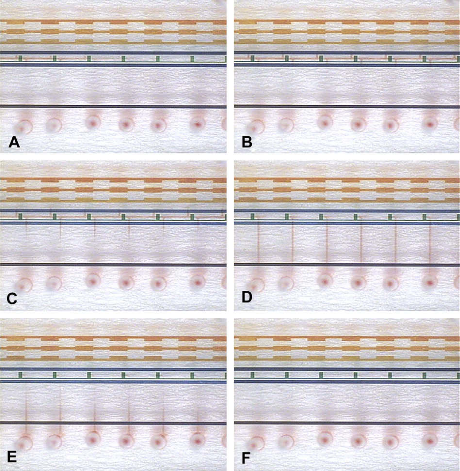
Steps of running the microfluidic device. For visualization, red food coloring solution is used instead of a real sample. (A) The sample is loaded and separated in the CE channel. (B) The fractionation valves are closed to form compartments in the CE channel so that the separated analytes are fractionated in the compartments. (C)–(F) The analyte fractions are transported into the fraction reservoirs by actuating the pump.

The analyte solution in each fraction reservoir is taken out by a home-made disposable dispensing tool and mixed with a MALDI matrix solution. The mixture is deposited on a MALDI target by a micropipette and dried in air. Thus, the analyte fractions are co-crystallized with the matrix on the MALDI target, ready for MALDI-MS. Two commercialized mass spectrometers are used for the study: Proteomics Analyzer 4700 produced by ABI (Foster City, CA) and PCS 4000 manufactured by Bio-Rad Laboratories (Hercules, CA). The correspondent MALDI targets were purchased from the same vendors.

Figure 3 shows the structure of the home-made disposable dispensing tool, which is composed of a tip made of fused-silica capillary, a fluid-storing chamber made of polyethylene tube, a connector, and a syringe. Pulling the syringe sucks the analyte solution from a fraction reservoir into the chamber. The analyte solution can be squeezed out by pushing the syringe. Compared with the micropipettes, this disposable dispensing tool is more effective because (1) the tip is easy to be inserted into the bottom of a fraction reservoir, and (2) the syringe is able to provide a strong sucking force. Although the syringe is over-pulled for obtaining a strong sucking force, a portion of analyte solution always wets the tip with airproof. This is due to the surface tension effects of an aqueous solution in the fused-silica capillary. Therefore, the analyte solution is not sucked into the syringe. This type of dispensing tool has the potential of serving as an interface between a microfluidic device and macroscale manipulation.

Figure 3.

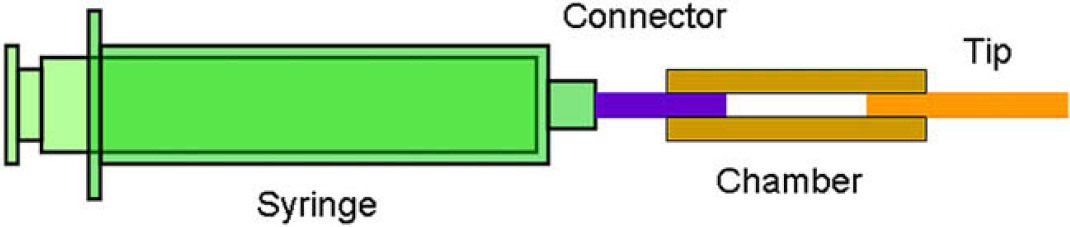
Structure of the home-made disposable dispensing tool.

Results and Discussion

Performance of the Microfluidic Device

Three factors influencing the performance of the microfluidic device were evaluated, including CE sample loading, CE separation efficiency, and MALDI sample preparation. The CE sample loading approach in the microfluidic device is a modification of the typical “double-T intersection” sample loading.³³ Pressure-driven flow is used to load the sample in the CE channel and a pair of valves is used to capture a sample plug. This type of sample loading is an alternative of the typical sample loading using EOF.³⁴ It is useful for the CE separation of biological samples that usually have high ionic strength. Figure 4A shows the layout of the modified “double-T” microfluidic device in which the stability of the sampling loading is tested, and Figure 4B shows the electropherogram obtained in it. The detection point is set at a distance to the intersection of sample-loading channel and CE channel, and the distance is defined as the effective length of CE. The reproducibility of the sample-loading process was observed at the detection point. The result gave a peak area variation of less than 5% in six consecutive sample-loading processes, showing excellent stability of this pressure-driven sample-loading method.

Figure 4.

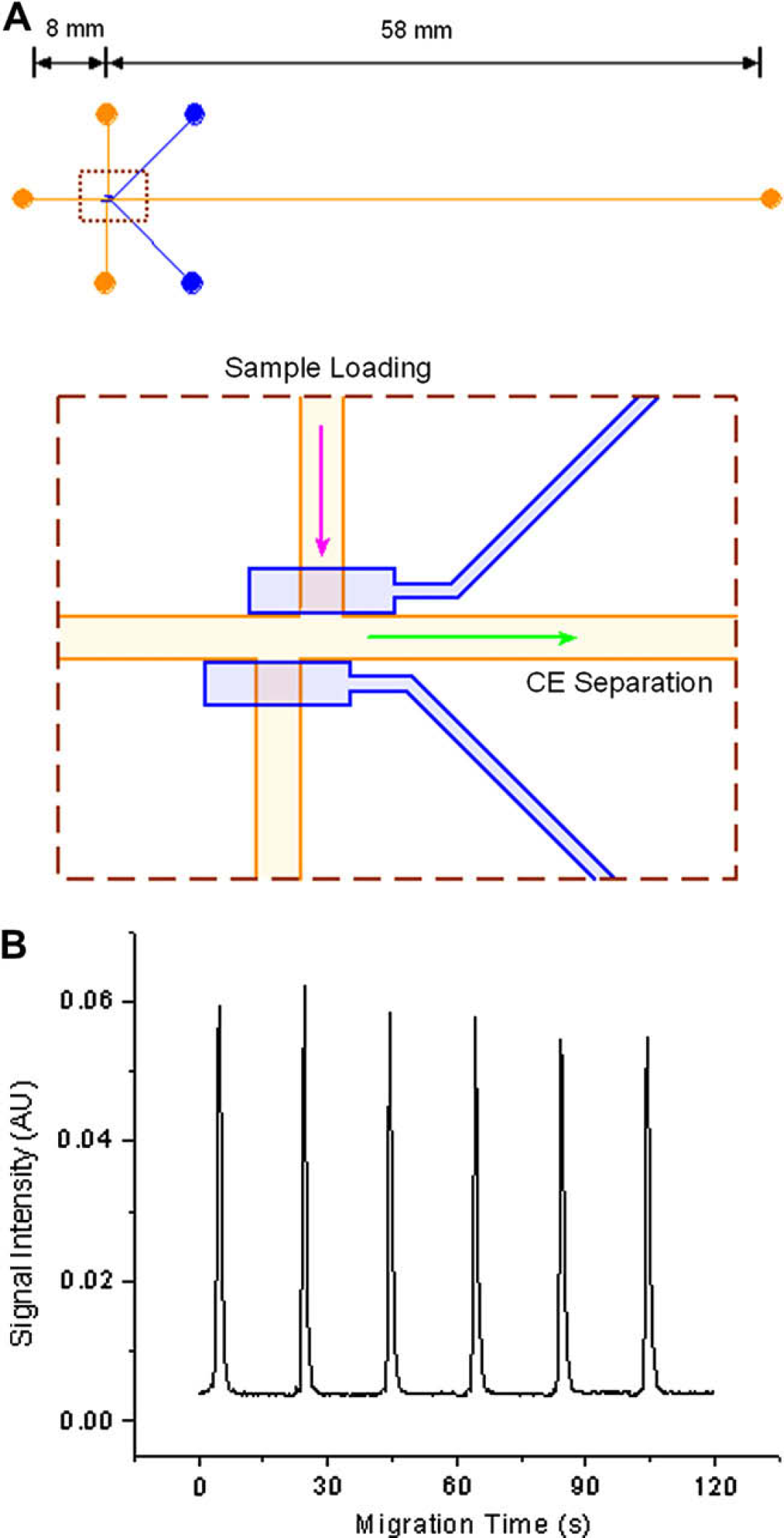
(A) Layout of the modified “double-T” microfluidic device. (B) Electropherogram obtained in the modified “double-T” microfluidic device. The effective length of CE is 3 mm. The electric field strength is ∼450 V/cm. The time of sample loading is 10 s. The laser-induced fluorescence (LIF) detection is carried out using a 633 nm He–Ne laser and a photomultiplier tube (PMT). The CE running buffer is 20 mM ammonium bicarbonate at pH 8.5 with 0.05% DDM and 0.005% SDS, and the sample is ∼0.1 μM AF647 dissolved in the CE running buffer.

The CE separation efficiency in the microfluidic device was compared with that in the modified “double-T” microfluidic device. According to the layout of the microfluidic device shown in Figure 1A, the connection of branch channels results in offsets along the CE channel when the horizontal valves are closed. The offsets change the flow profile of EOF to result in peak broadening and tailing effect, which lower the separation efficiency. Figure 5 shows the comparison of the CE separation of a standard sample in the two microfluidic devices. Using the first peak as an example, the theoretical plate number in Figure 5A is ∼15 times higher than that in Figure 5B. However, considering the peak capacity of ∼5 estimated from the third peak in Figure 5B, the separation efficiency in the microfluidic device is sufficient for the samples having a small number of analytes.

Figure 5.

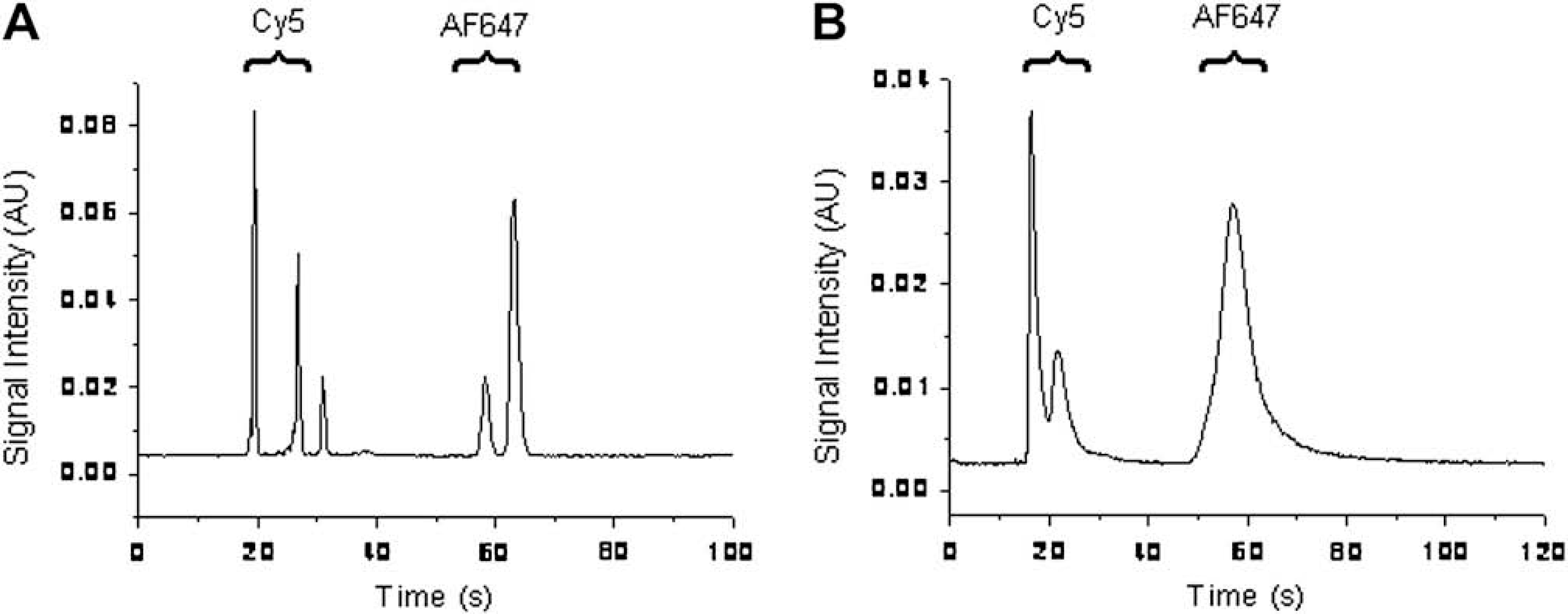
(A) Electropherogram obtained in the modified “double-T” microfluidic device. (B) Electropherogram obtained in the microfluidic device for coupling CE and MALDI-MS. In both microfluidic devices, the effective length of CE is 35 mm. The electric field strength is ∼450 V/cm. The time of sample loading is 10 s. The LIF detection is carried out using a 633 nm helium–neon laser and a PMT. The CE running buffer is 20 mM ammonium bicarbonate at pH 8.5 with 0.05% DDM and 0.005% SDS, and the sample is ∼0.1 μM Cy5 and ∼0.3 μM AF647 dissolved in the CE running buffer. Multiple peaks of Cy5 and AF647 are shown probably because hydrolysis of each fluorescent reagent in the CE running buffer produced a variety of products.

Two-Step Analysis of Samples

An experiment was implemented to verify the capability of the microfluidic device. In this experiment, a mixture composed of standard peptides NRT (average mass, 1673.0) and FPB (average mass, 1570.6) was used as the sample. These peptides are easily ionized in MALDI-MS so that high sensitivity is usually achievable. The peptides were dissolved in the CE running buffer with each peptide at a concentration of 1 mg/mL. After loading the sample in the CE channel, the CE separation of the two analytes was carried out. In regular free-solution CE each analyte migrates at a specific mobility, and the mobility difference results in the separation of analytes. Usually the electroosmotic mobility of CE running buffer is more significant than the electrophoretic mobility of analytes, so that all analytes are carried in EOF from anode to cathode. Therefore, the overall mobility of an analyte is close to the electroosmotic mobility, especially for that having a low charge number. The electroosmotic mobility is used to estimate the needed time of CE separation. In practice, the current-monitoring method was used to measure the EOF velocity before the CE separation,³⁵ and the time of CE separation was set to be short enough so that EOF should not exceed the rightmost branch channel. The exact time of CE separation was adjusted by trial-and-error to realize the goal of having most of the separated analytes within the two outermost branch channels for an efficient fractionation. Then the analyte fractions were transported into the fraction reservoirs together with the channel-filling fluid to reach a total volume of ∼1 μL. The analyte solution was taken out of each fraction reservoir and mixed with 0.8 μL 2.5 mg/mL CHCA in 1/1 acetonitrile–water containing 0.1% trifluoroacetic acid. The mixture was deposited on a stainless steel MALDI target. The analyte fractions were dried on the MALDI target to become solid crystallized MALDI sample spots, which were analyzed by the Proteomics Analyzer 4700 mass spectrometer. The MALDI target was then cleaned and polished for reuse.

In this article, signal intensity of an analyte is measured as the peak area of that analyte in a mass spectrum. In MALDI sample preparation, the heterogeneity of crystallization results in spot-to-spot variation of ionization rate of the same analyte. Thus the absolute signal intensity of analyte in a MALDI mass spectrum is not necessarily related to its quantity in the MALDI sample spot.^{36
–38} To overcome this disadvantage, BRK was used as an internal standard to calibrate the signal intensity of analytes. The internal standard was added to the CE running buffer and distributed evenly in the CE channel. The quantity of BRK should remain the same in all analyte fractions. However, the signal intensity of BRK changed significantly among the MALDI sample spots because of (1) possible fluid loss in transferring the analyte solution and (2) the spot-to-spot variation of ionization rate. Assuming these two effects impact the signal intensity of all analytes in the same way, the signal intensity of BRK can be used to compensate the variation resulted from these two effects. Therefore, the quantity of analytes in each analyte fraction is represented by the signal intensity ratio of the analytes to the internal standard. This calibration produces relative signal intensity which represents absolute quantity of analytes. By applying the quantitation method in all MALDI sample spots, the quantity change of the analytes among all analyte fractions is obtained. Thus an electropherogram is established by plotting the relative signal intensity of analytes to the position of analyte fractions. The position of analyte fractions is represented by the fraction reservoir number. The signal intensity was measured in Proteomics Analyzer 4700 Software and the quantitation was realized in Origin produced by OriginLab (Northampton, MA). To determine the precision of the quantitation method, the sample was first diluted in the CE running buffer and then in the channel-filling fluid to create a reference solution with a similar composition to the analyte fractions. The reference solution was deposited on a series of MALDI sample spots, which were analyzed by the same mass spectrometer. The relative signal intensity of analytes was obtained using the quantitation method. Theoretically the relative signal intensity of each analyte should be the same among all MALDI sample spots. But in fact the variation still exists at a low level. It is probably because each analyte has a slightly different profile for the spot-to-spot variation of ionization rate. Therefore, relative standard deviation of the relative signal intensity is measured for each analyte as the degree of uncertainty, which is applied to the relative signal intensity of that analyte in the electropherogram obtained from the two-step analysis.

Dilution of analytes is a result of transporting the analyte fractions into the fraction reservoirs together with the channel-filling fluid. However, after the fraction solution is deposited on the MALDI target, the dilution is counteracted by the concentration resulted from the evaporation of solvents. For a particular MALDI sample spot, the signal intensity of an analyte is dependent on its quantity rather than its concentration in the analyte solution. Therefore, the dilution does not significantly influence the signal intensity of analytes.

Figure 6 shows the experimental result of the mixture of NRT and FPB: Figure 6A shows three examples of the signals obtained from the MALDI sample spots, and Figure 6B shows the electropherogram obtained from the two-step analysis. The CE separation of NRT and FPB is observed in the electropherogram. The analyte peaks are not perfectly symmetric, due to the peak tailing effect caused by the offsets along the CE channel. The CE separation of analytes is explained by the mobility difference: (1) the two analytes have similar masses so that the sizes are close; and (2) at pH 8.5, NRT (calculated isoelectric point, ∼9.5) is slightly positively charged, whereas FPB (calculated isoelectric point, ∼3.9) is strongly negatively charged. The charge number difference results in the mobility difference. Because the analytes are carried in EOF from anode to cathode, the positively charged NRT migrates faster than the negatively charged FPB, as shown in Figure 6B.

Figure 6.

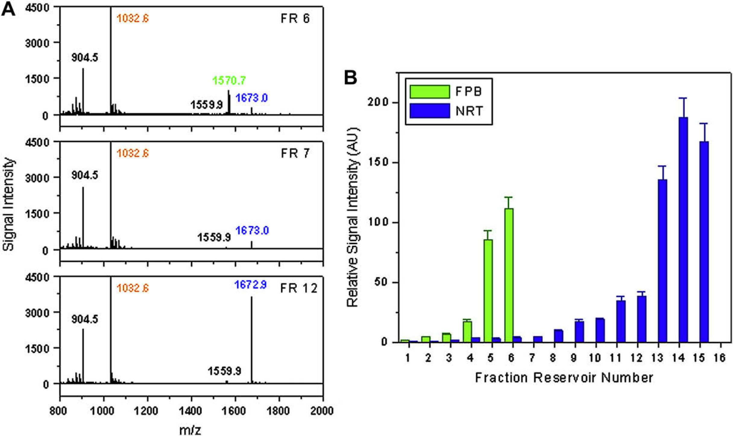
Two-step analysis of the mixture of NRT and FPB. (A) The signals obtained from the MALDI sample spots for the analyte solution in fraction reservoirs 6, 7, and 12. The fraction reservoirs are numbered from left to right, referring to the layout shown in Figure 1A. The fraction reservoir number represents the position of the analyte fractions. The laser energy in the Proteomics Analyzer 4700 was set at 2600 V. The peaks of NRT, FPB, and BRK are labeled in blue, green, and orange, respectively. The diagrams show the quantity change of NRT and FPB in the analyte solution from different fraction reservoirs. (B) Electropherogram of the CE separation established by plotting the relative signal intensity of analytes to the position of analyte fractions. Because the absolute signal intensity of FPB is much smaller than that of NRT, the relative signal intensity of FPB in all MALDI sample spots is multiplied by 10 to display the two analyte peaks with comparable heights.

Because CE separation is based on the mobility difference of analytes, it is useful for separating structural analogs with charge number difference, such as phosphopeptide isomers.^39,40 Another experiment was implemented to extend the application of the microfluidic device. In this experiment, a mixture composed of PS1 (average mass 1209.3) and DP-PS1 (average mass, 1129.3) was used as the sample. PS1 is a natural phosphopeptide and DP-PS1 is the dephosphorylated form of PS1. The peptides were dissolved in the CE running with each peptide at a concentration of 1 mg/mL. The manipulation protocol of CE separation, fractionation, and fraction transport remained the same as that in the previous experiment. After the fraction transport, the analyte solution was taken out of each fraction reservoir and mixed with 1 μL 20 mg/mL DHB in 1/1 acetonitrile–water containing 1.5% phosphoric acid. The mixture was deposited on an NP20 MALDI target manufactured by Bio-Rad Laboratories. The analyte fractions were dried on the MALDI targets to become solid crystallized MALDI sample spots, which were analyzed by the PCS 4000 mass spectrometer. Each mass spectrum was exported and the signal intensity of analytes was measured in Origin. The quantitation method used in the previous experiment was also used in this experiment and an electropherogram is established by plotting the relative signal intensity of analytes to the position of analyte fractions.

Figure 7 shows the experimental result of the mixture of PS1 and DP-PS1: Figure 7A shows three examples of the signals obtained from the MALDI sample spots, and Figure 7B shows the electropherogram obtained from the two-step analysis. In the electropherogram, it is observed that the CE separation of PS1 and DP-PS1 is effective. The CE separation of analytes is explained by the mobility difference resulted from the charge number difference: at pH 8.5, PS1 (calculated isoelectric point ∼4.6) is strongly negatively charged, whereas DP-PS1 (calculated isoelectric point ∼8.4) is almost neutral. Because the analytes are carried in EOF from anode to cathode, the almost neutral DP-PS1 migrates faster than the negatively charged PS1, as shown in Figure 7B.

Figure 7.

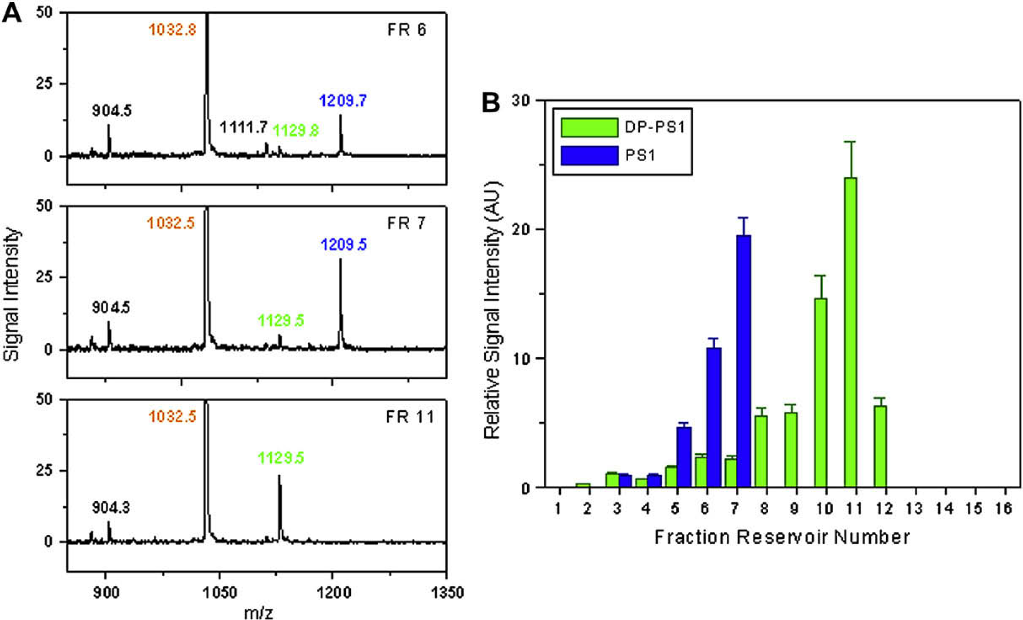
Two-step analysis of the mixture of PS1 and DP-PS1. (A) The signals obtained from the MALDI sample spots for the analyte solution in fraction reservoirs 6, 7, and 11. The laser energy in the PCS 4000 was set at 3000 nJ. The peaks of PS1, DP-PS1, and BRK are labeled in blue, green, and orange, respectively. The diagrams show the quantity change of PS1 and DP-PS1 in the analyte solution from different fraction reservoirs. (B) Electropherogram of the CE separation established by plotting the relative signal intensity of analytes to the position of analyte fractions.

Conclusion

The two-step analysis achieved in both experiments shows that the microfluidic device is as an excellent platform for coupling CE and MALDI-MS. The miniaturized functionality is essential for the performance of the microfluidic device. It facilitates the formation of nanoliter-scale analyte fractions, which enable convenient analyte transport for MALDI sample preparation. In a larger scope, the microfluidic device is the first to use built-in actuators for coupling CE and MALDI-MS. It broadens the application of a microfluidic device with actuators in the field of coupling chromatography and MS.

There are potential improvements for increasing the performance of the microfluidic device. According to the mechanism of fractionation, the number of analyte fractions decides the x-axial resolution of the electropherogram obtained from two-step analysis. It is because the analytes in each analyte fraction are mixed in the corresponding analyte solution after the fraction transport. Because of the mixing, averaged quantity of analytes is measured in each analyte fraction, so that the result of CE separation within each compartment is eliminated. Thus the electropherogram is fragmented along the x-axis by the number of analyte fractions. For the CE channel with a fixed length, the x-axial resolution of the electropherogram is dependent on the length of each compartment. Although the length may be decreased, it is restricted by two factors. First, the compartments must have enough volume so that the analyte fractions captured therein provide adequate analytes for MALDI-MS. This factor is related to the sensitivity of MALDI-MS, and it is not significant if the mass spectrometer has very low limit of detection. Second, the fraction reservoirs must keep a certain distance in between for device fabrication. It restrains the distance between the branch channels as well as the length of the compartments. This aspect can be slightly improved by staggered positioning of the fraction reservoirs. Alternatively, the number of compartments can be increased by elongating the CE channel while the length of each compartment is maintained. This approach may also enhance the peak capacity as well as the CE separation efficiency. However, it increases the size of the microfluidic device and the amount of manual work involved in transferring the analyte solution at the same time.

The total time needed for the two-step analysis is relatively long due to the ∼1 h pumping time for transporting ∼1 μL analyte solution into the fraction reservoirs. The volume of analyte solution is mainly contributed by the channel-filling fluid. If the analyte fractions are directly transported from the microfluidic device to the MALDI target, the volume may be substantially reduced because the relatively large volume is not needed for transferring the analyte solution out of the microfluidic device. To realize this goal, the MALDI target should be customized so that it can be assembled with the microfluidic device. The design of the microfluidic device may be modified at the same time to facilitate an efficient integration with the MALDI target. For example, small pores can be fabricated to directly connect the branch channels to the sample-deposition areas on the MALDI target. This approach not only accelerates the two-step analysis but reduces the size of MALDI sample spots. By decreasing the size of MALDI sample spots, the ionization rate of analytes should be enhanced because the analytes have higher surface density and are more accessible by the laser beam in a mass spectrometer. Therefore, the signal intensity of analytes may increase if the integration of microfluidic device and MALDI target is achieved.

References

Greis

K. D.

Mass spectrometry for enzyme assays and inhibitor screening: An emerging application in pharmaceutical research. Mass Spectrom. Rev. 2007, 26, 324–339.

Yates

J. R.

Mass spectrometry and the age of the proteome. J. Mass Spectrom. 1998, 33, 1–19.

Mann

Hendrickson

R. C.

Pandey

Analysis of proteins and proteomes by mass spectrometry. Annu. Rev. Biochem. 2001, 70, 437–473.

Griffiths

W. J.

Jonsson

A. P.

Liu

Rai

D. K.

Wang

Electro-spray and tandem mass spectrometry in biochemistry. Biochem. J. 2001, 355, 545–561.

Mirsaleh-Kohan

Robertson

W. D.

Compton

R. N.

Electron ionization time-of-flight mass spectrometry: Historical review and current applications C. Mass Spectrom. Rev. 2008, 27, 237–285.

C. C.

Yates

J. R.

The application of mass spectrometry to membrane proteomics. Nature Biotech. 2003, 21, 262–267.

Murray

K. K.

Coupling matrix-assisted laser desorption/ionization to liquid separations. Mass Spectrom. Rev. 1997, 16, 283–299.

Cai

Henion

Capillary electrophoresis-mass spectrometry. J. Chromatogr. A 1995, 703, 667–692.

Novotny

M. V.

Mechref

New hyphenated methodologies in high-sensitivity glycoprotein analysis. J. Sep. Sci. 2005, 28, 1956–1968.

10.

Lee

M. S.

Kerns

E. H.

LC/MS applications in drug development. Mass Spectrom. Rev. 1999, 18, 187–279.

11.

Xie

Miao

Shih

Tai

Lee

T. D.

Microfluidic platform for liquid chromatography—tandem mass spectrometry analyses of complex peptide mixtures. Anal. Chem. 2005, 77, 6947–6953.

12.

Yin

Killeen

Brennen

Sobek

Werlich

van de Goor

Microfluidic chip for peptide analysis with an integrated HPLC column, sample enrichment column, and nanoelectrospray tip. Anal. Chem. 2005, 77, 527–533.

13.

Wen

Lin

Xiang

Matson

D. W.

Udseth

H. R.

Smith

R. D.

Microfabricated isoelectric focusing device for direct electrospray ionization-mass spectrometry. Electrophoresis 2000, 21, 191–197.

14.

Zhang

Foret

Karger

B. L.

High-throughput microfabricated CE/ESI-MS: Automated sampling from a microwell plate. Anal. Chem. 2001, 73, 2675–2681.

15.

Wall

D. B.

Berger

S. J.

Finch

J. W.

Cohen

S. A.

Richardson

Chapman

Drabble

Brown

Gostick

Continuous sample deposition from reversed-phase liquid chromatography to tracks on a matrix-assisted laser desorption/ionization precoated target for the analysis of protein digests. Electrophoresis 2002, 23, 3193–3204.

16.

Ericson

Phung

Q. T.

Horn

D. M.

Peters

E. C.

Fitchett

J. R.

Ficarro

S. B.

Salomon

A. R.

Brill

L. M.

Brock

An automated noncontact deposition interface for liquid chromatography matrix-assisted laser desorption/ionization mass spectrometry. Anal. Chem. 2003, 75, 2309–2315.

17.

K. W.

Liu

Knapp

D. R.

Plastic microchip liquid chromatography-matrix-assisted laser desorption/ionization mass spectrometry using monolithic columns. J. Chromatogr. A 2006, 1111, 40–47.

18.

Zhan

Gusev

Hercules

D. M.

A novel interface for on-line coupling of liquid capillary chromatography with matrix-assisted laser desorption/ionization detection. Rapid Commun. Mass Spectrom. 1999, 13, 2278–2283.

19.

Wei

Nolkrantz

Parkin

M. C.

Chisolm

C. N.

O'Callaghan

J. P.

Kennedy

R. T.

Identification and quantification of neuropeptides in brain tissue by capillary liquid chromatography coupled off-line to MALDI-TOF and MALDI-TOF/TOF-MS. Anal. Chem. 2006, 78, 4342–4351.

20.

Johnson

Bergquist

Ekman

Nordhoff

Schurenberg

Kloppel

Muller

Lehrach

Gobom

A CE-MALDI interface based on the use of prestructured sample supports. Anal. Chem. 2001, 73, 1670–1675.

21.

Page

J. S.

Rubakhin

S. S.

Sweedler

J. V.

Direct cellular assays using off-line capillary electrophoresis with matrix-assisted laser desorption/ionization time-of-flight mass spectrometry. Analyst 2000, 125, 555–562.

22.

Musyimi

H. K.

Guy

Narcisse

D. A.

Soper

S. A.

Murray

K. K.

Direct coupling of polymer-based microchip electrophoresis to online MALDI-MS using a rotating ball inlet. Electrophoresis 2005, 26, 4703–4710.

23.

Liu

Tseng

Garcia

Lebrilla

C. B.

Mukerjee

Collins

Smith

Electrophoresis separation in open microchannels. A method for coupling electrophoresis with MALDI-MS. Anal. Chem. 2001, 73, 2147–2151.

24.

Little

M. W.

Murray

K. K.

Interfacing capillary gel microfluidic chips with infrared laser desorption mass spectrometry. J. Am. Soc. Mass Spectrom. 2006, 17, 469–474.

25.

Loo

Ogorzalek R. R.

Cavalcoli

J. D.

Van Bogelen

R. A.

Mitchell

Loo

J. A.

Moldover

Andrews

P. C.

Virtual 2-D gel electrophoresis: Visualization and analysis of the e. coli proteome by mass spectrometry. Anal. Chem. 2001, 73, 4063–4070.

26.

DeVoe

D. L.

Lee

C. S.

Microfluidic technologies for MALDI-MS in proteomics. Electrophoresis 2006, 27, 3559–3568.

27.

Foret

Kusy

Microfluidics for multiplexed MS analysis. Electrophoresis 2006, 27, 4877–4887.

28.

Koster

Verpoorte

A decade of microfluidic analysis coupled with electrospray mass spectrometry: An overview. Lab Chip 2007, 7, 1394–1412.

29.

Unger

M. A.

Chou

H. P.

Thorsen

Scherer

Quake

S. R.

Monolithic microfabricated valves and pumps by multilayer soft lithography. Science 2000, 288, 113–116.

30.

Huang

Zare

R. N.

Construction of microfluidic chips using polydimethylsiloxane for adhesive bonding. Lab Chip 2005, 5, 1393–1398.

31.

Luo

Zare

R. N.

Microfluidic device for immunoassays based on surface plasmon resonance imaging. Lab Chip 2008, 8, 694–700.

32.

Huang

Kim

Zare

R. N.

Coating of poly(dimethylsiloxane) with n-Dodecyl-β-D-Maltoside to minimize nonspecific protein absorption. Lab Chip 2005, 5, 1005–1007.

33.

Blas

Delaunay

Rocca

Electrokinetic-based injection modes for separative microsystems. Electrophoresis 2008, 29, 20–32.

34.

Jensen

Gamby

Bai

Girault

H. H.

A flexible sample introduction method for polymer microfluidic chips using a push/pull pressure pump. Lab Chip 2004, 4, 512–515.

35.

Huang

Gordon

M. J.

Zare

R. N.

Current-monitoring method for measuring the electroosmotic flow rate in capillary zone electrophoresis. Anal. Chem. 1988, 60, 1837–1838.

36.

Nelson

R. W.

McLean

M. A.

Hutchens

T. W.

Quantitative determination of proteins by matrix-assisted laser desorption/ionization time-of-flight mass spectrometry. Anal. Chem. 1994, 66, 1408–1415.

37.

Muddiman

D. C.

Gusev

A. I.

Langner

K. S.

Proctor

Hercules

D. M.

Tata

Venkataramanan

Diven

Simultaneous quantification of cyclosporin A and its major metabolites by time-of-flight secondary-ion mass spectrometry and matrix-assisted laser desorption/ionization mass spectrometry utilizing data analysis techniques: Comparison with high-performance liquid chromatography. J. Mass Spectrom. 1995, 30, 1469–1479.

38.

Chatman

Harris

Siuzdak

An automated MALDI mass spectrometry approach for optimizing cyclosporin extraction and quantitation. Anal. Chem. 1997, 69, 3767–3771.

39.

Ballard

J. N. M.

Lajoie

G. A.

Yeung

K. K.

Selective sampling of multiply phosphorylated peptides by capillary electrophoresis for electrospray ionization mass spectrometry analysis. J. Chromatogr. A 2007, 1156, 101–110.

40.

Tadey

Purdy

W. C.

Capillary electrophoretic resolution of phosphorylated peptide isomers using micellar solutions and coated capillaries. Electrophoresis 1995, 16, 574–579.

Microfluidic Device for Coupling Capillary Electrophoresis and Matrix-Assisted Laser Desorption Ionization-Mass Spectrometry

Abstract

Keywords

Introduction

Experimental

Chemicals and Reagents

Design and Fabrication of the Microfluidic Device

Running the Microfluidic Device

Results and Discussion

Performance of the Microfluidic Device

Two-Step Analysis of Samples

Conclusion

References