
Abstract
This article briefly describes the system for optical coherence tomography (OCT), an interferometric imaging technique and focuses on software controlling of this complex apparatus and data acquisition (DAQ) by means of LabVIEW. It states advanced LabVIEW techniques for parallel DAQ, multi-instrument communication, and postprocessing needed to assure OCT measurements being carried out at the University of Oulu.
Introduction
The aim of this project was to develop a software for an experimental system for ultra-high-resolution optical coherence tomography (OCT) at the University of Oulu (Finland). The laboratory research was focused on the use of the mentioned technique for measuring inner and surface structure of paper. 1 –5
Paper industry is highly developed in the Northern Europe and asks for advanced evaluation methods of manufactured products. The reason may especially be to reach the end-users' specifications at the lowest cost. Next is the optimal structure and surface quality of produced paper. Parameters such as roughness influence properties of paper such as gloss or ink absorption. Ecological aspect also plays an important role.
Most of the commercial instruments are focused on only one property of the paper, for example, with common optical glossmeters one is able to measure an average gloss. It is possible to estimate roughness parameters by means of technology where the amount of air passed between the sample and the measuring head is measured (the so-called air-leak methods). Nevertheless, this technology is prone to failure because the paper usually contains apertures which inevitably influence the measurement. Moreover, to cover all grades of paper from rough base paper to highly coated photo paper one instrument is generally not enough. OCT offers complex information, namely, topographic, tomographic, roughness, and so on. All these are from one measurement and based only on proper processing of acquired data. In addition, OCT is a noninvasive and noncontact technique.
Optical Coherence Tomography
OCT is rather a young technique of imaging subsurface structure of subjects, nowadays, with a resolution <1 μm. Originally, it was used only to study human tissues (widely used in modern ophthalmology), but it also finds its place in industrial sector at present.
OCT is based on low coherence interferometry (LCI). In conventional interferometry with long coherence length, interference of light occurs over a distance of meters. In OCT, this interference is shortened to a distance of micrometers, thanks to the use of wide bandwidth light sources that can emit the light over a broad range of wavelengths. Round-trip coherence length of sources which have Gaussian-shaped spectrum or resembles it (typically superluminescent diodes [SLDs]) and thereby the axial resolution of the system is given by the formula:
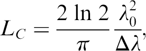
where Δλ is the full width at half maximum (FWHM) wavelength range of the light source and λ 0 is the central wavelength. In case of light sources with complex-shaped spectrum, the coherence length has to be measured. Transversal resolution of the system is given by the focusing optics:
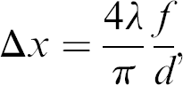
where f is the focal length of focusing lens and d is the light diameter on the lens.
Commonly used broadband light sources used in OCT are SLDs. Generally, they obtain a spectrum width of a few tens of micrometers and an axial resolution around 10 μm. Also lasers with extremely short pulses (femtosecond lasers) can be used to generate partially coherent light.
The aim of this work is not to explain the theory of LCI or OCT in detail, wherefore, only simplified schema (Fig. 1) is stated and basic principles are outlined. For a closer look, see the literature (Refs. 6–8).
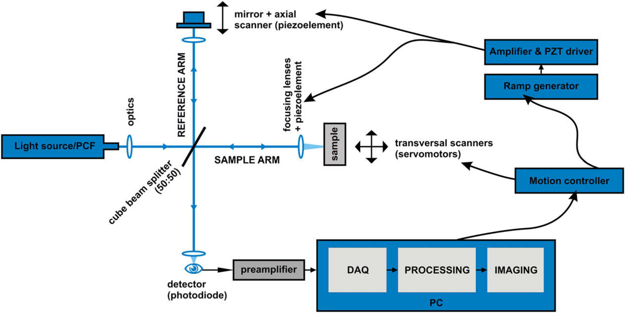
Schema of the apparatus for OCT.
Schema
The experimental system consists of Ti:sapphire femtosecond laser and nonlinear fiber, Photonic Crystal Fiber (PCF), as a light source. The Ti:sapphire laser has central wavelength of 800 nm, FWHM 10–30 nm, pulse duration of 50–80 fs and repetition rate of 80 MHz. Output of the laser is focused in the PCF and due to nonlinear optical phenomena such as self-phase modulation, Raman scattering, and four-wave mixing, widening of the spectra occurs with small energy while high spatial coherence is preserved. 9 This widening of spectrum is called supercontinuum generation. The output of the PCF where wavelengths from 450 to 1700 nm are present is collimated and can be further modified by optical filters to adjust the most suitable spectra. 10,11 The resulting beam is focused on Michelson type interferometer. It consists of beam splitter (50:50) where the beam is split into two arms—a reference arm and an arm with a sample. A mirror is located at the end of the reference arm attached to a scanner which ensures its axial motion.
The property of LCI is that the interference occurs only if the path difference is less than the coherent length of the light source. This interference is called cross-correlation (if the arms are identical, then autocorrelation). The envelope of this modulation changes as the path difference of the split beams differs and its peak presents the point where both beams traveled the same distance. In most cases of OCT, the autocorrelation function has the Gaussian shape (it is given by the spectra of the light source).
The motion of the mirror serves for the depth regulation, at the same time shifts the useful signal to Doppler frequency which is dependent on the velocity of the scanner. Doppler frequency is expressed as follows:
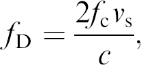
where f c is the central optical frequency of the source, v s is the speed of the scanner and c is the speed of light.
Piezonanopositioners P-783 by Physik Instrument are used as scanners along with E-665 controller. Nevertheless, for the creation of the voltage ramp for piezoelectric (PZT) elements, external signal generator was constructed. Its output is further amplified by the E-665 controller which drives the motion of the PZT elements by means of a feedback loop. An external generator of voltage ramp was developed because E-665 did not ensure enough stable and linear output with higher repetition rates.
The arm with the sample is also equipped with piezonano-positioner which holds a focusing lens and copies the motion of the first PZT element so that the narrowest part of the beam is always focused on the just-measured part of the sample. The sample itself is placed on xy linear stage (Newport UMR8.25) with two actuators (Newport CMA-25) controlled by Newport ESP 300 (universal motion controller) to provide scanning in transversal directions to obtain two-dimensional and three-dimensional images.
Reference beam and the beam from the sample reflect back, pass again through the beam splitter, and merge in the silicon diode (sensing wavelengths from 400 to 1100 nm). Analog signal from the photodiode is then passed through a transimpedance amplifier, specially designed for OCT, providing strong signal at the output and high signal-to-noise ratio. This output is then directed to an adapter (NI BNC-2110) of DAQ card and next to a PC where the signal is digitalized.
Architectures Used for the Software Creation
Data Acquisition
Demands for the data acquisition (DAQ) were as follows; to acquire the photodiode signal for 80 ms with a sampling frequency of F s = 100 kHz each time the trigger impulse appears, which is approximately every 100–150 ms (according to the settings). Eighty milliseconds covers the time when the nanopositioners set the beam into the start position and with constant velocity make the scan. The first 20 ms of the signal has to be cut off because this represents the nonlinear part of the driving voltage ramp—velocity is not constant, nanopositioners are being aligned to the start position. The linear part converted from voltage to position is shown in Figure 2.
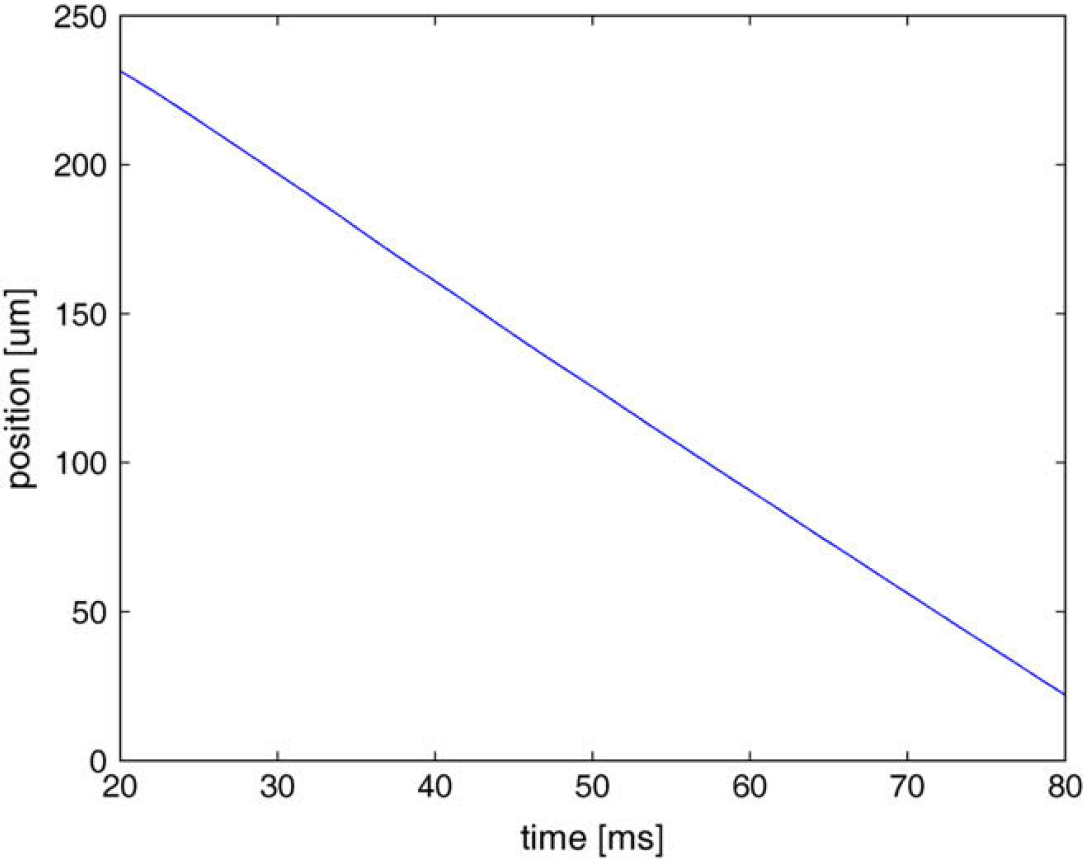
Course of PZT position in dependence of time.
For calculating the depth of the measurement, it is necessary to know the velocity of the scanners. It can be determined by converting the voltage ramp to the position coordinates, followed by a numeric derivative in the linear part. During our measurements, this value was 3.51 mm/s. The resulting depth is given by the formula:
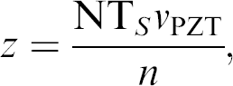
where N is the number of samples over scanned area, T s is the sampling period (T s = 1/F s), V PZT is the velocity of nanopositioners, and n is the refraction index of the material under examination.
A 12-bit DAQ card NI-6110 and BNC adapter BNC-2110 are used for DAQ, where the output from the photodiode is connected to one channel and the trigger signal to PFI0.
There are two ways to perform retriggerable DAQ with cards of this family by National Instruments. The first way is outlined in Figure 3 which represents a part of the code in LabVIEW.
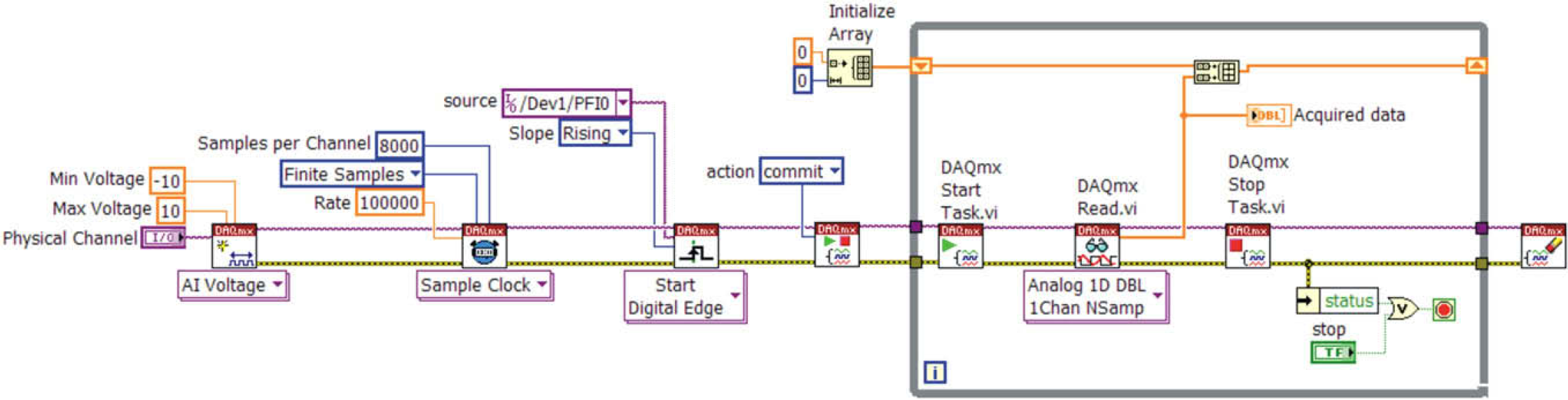
Software-driven retriggerable DAQ.
First, a new channel is created and configured for voltage measurement. Next, sampling frequency, amount of samples, and sampling mode (finite number of samples) are set. In the next step, the connector for trigger signal is specified plus whether the measurement should begin with rising or falling edge. The items are then passed to the DAQ card which sets its hardware according to the specified actions. When the trigger appears, the measurement starts, data are acquired, and the reading is terminated. On the next trigger, the situation repeats—the measurement is started again, the data are acquired, and so on. This means that after each trigger, the card is software-reconfigured and the task restarted. This solution is suitable for slow processes. The time taken is longer and non-constant and depends on the performance of the computer and its present workload. We used this approach in our application in the beginning. Nevertheless, it turned out that after some time, when the application is tasked along with the processing of the measured data or in case any other Windows process takes up significant CPU time, there are delays in the card circuit reconfiguration during restarting of the DAQ, and as a consequence, some trigger signals are omitted. Thus, corresponding data are not acquired. This was unacceptable.
Therefore, a second method was applied. The card counter is used to generate pulse train which acts as an external sample clock. It is possible to retrigger counters and thereby the necessity to start and stop them drops out and hence the delays. This solution is shown in Figure 4.
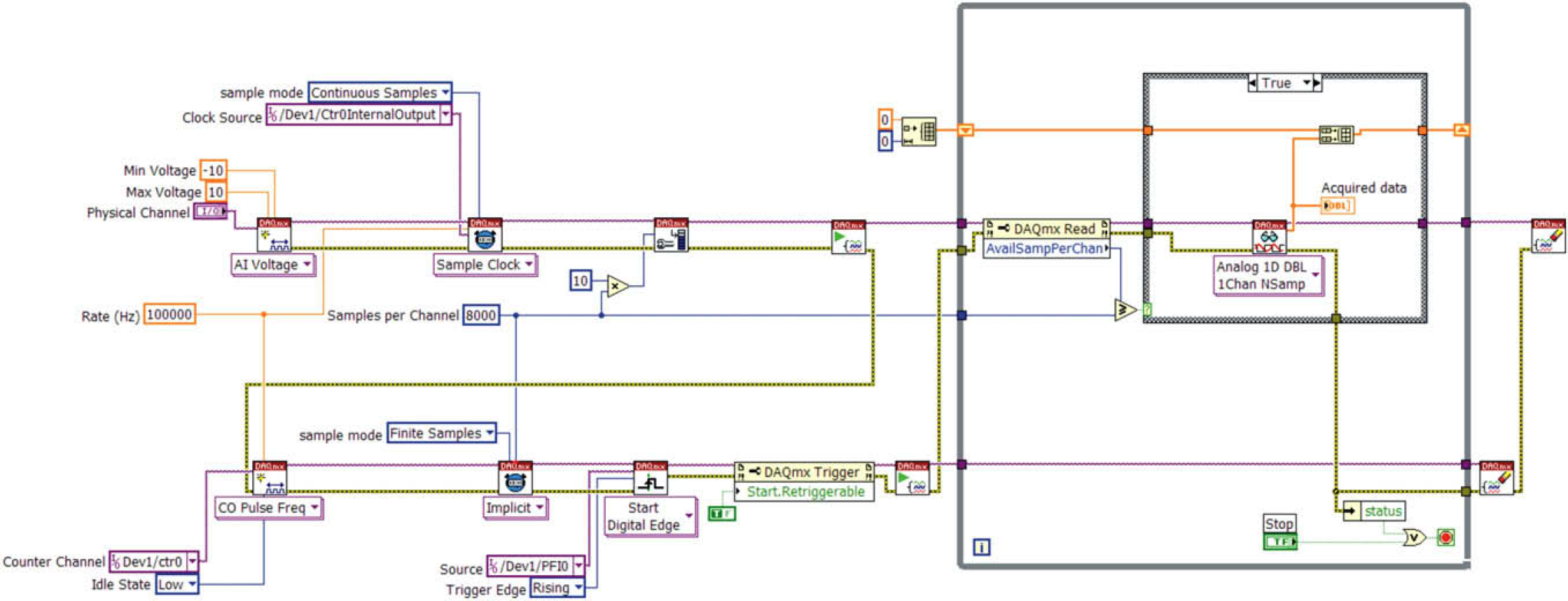
Retriggerable DAQ using counter.
Everything starts again with configuration of the measurement channel and this time with setting “external” sampling source from the inner output of the counter. Next, the buffer size is set, which is better to create larger, in case the application would not finish data reading from the card memory and meanwhile new trigger impulse appeared, which would fill up the buffer with newly acquired data. Along with the above-mentioned factors, the counter channel is created to produce a series of pulses of given frequency (i.e., frequency to sample acquired signal). Subsequently, the pulse count which should be produced with rising edge of each trigger is set. This operation is set as retriggerable.
State Machine
Each technical application can be described with more or less complicated state diagram. The architecture of State Machine (SM) can be used to implement complex decision-making algorithms represented by state diagrams or flow-charts. 12 Each state performs something different and specific, and after applying the decision-making logic, it unambiguously leads to one or more states. The output function is thus determined by the current state alone. This matches the Moore machine.
The state approach is one of the advanced and often-used programming techniques in LabVIEW. Besides its ability to implement decision-making algorithms, SMs offer efficient planning. They are relatively easy to create and rather easy to modify just by adding or removing particular states or by changing their functionality. On the other hand, the creator of each application should not, especially in case of complicated SM, underestimate the necessity of designing the state diagram. This can be achieved while using pen and paper or, in case of LabVIEW, with the use of utilities such as State Chart Module, based on Unified Modeling Language.
To represent the state diagram in LabVIEW, we need at least the following programming structures:
While loop—ensures the transition to other state.
Case structure—each case contains a code which is executed for a given state.
Shift register—transfers information about next/current state.
Decision-making logic—determines the next state.
LabVIEW programming is specific compared with text-based programming languages. We decided to use easy-to-understand examples to describe architectures that we have used, but we also presume that there is a basic knowledge of LabVIEW programming.
The simplest example of SM is presented in Figure 5; 1 labels While loop, 2 points at Shift register, which transfers the information about the next state. It is preset at the beginning so that after the start of the program, it proceeds into the “Initialize” state (3). In this state, the number 4 marks the determination of the next state by inserting a state. In this case, it is state “A,” but it could also be any of the other available states (5).
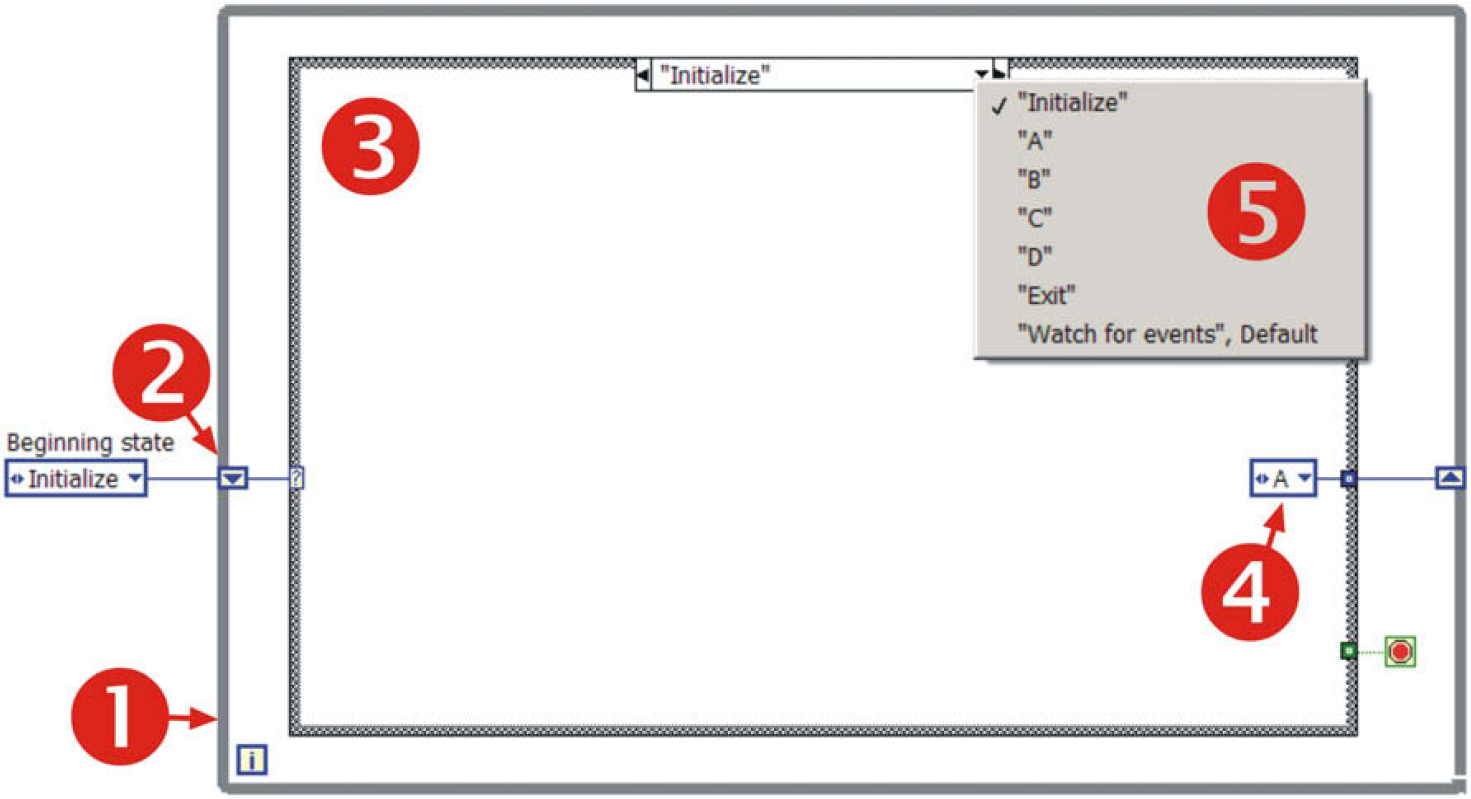
Example of SM.
State named “Watch for events” (Fig. 6) contains the so-called Event structure (6) to handle the events caused by the user, which may request execution of appropriate states—in this simple example, it is only the termination of the application (state “Exit”).
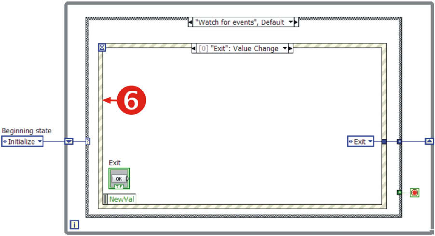
SM, event structure for handling events caused by a user.
For more detail on SM see Ref. 13.
Queued State Machine
SM architecture is universal; nevertheless, it has its limits. If the volume of a project expands, it is not easy to force the SM to perform all the requisite operations. In such a situation, it is efficient to resort to the so-called Queued State Machine (QSM).
Notation for describing the characteristics of a queuing model was first suggested by David G. Kendall in 1953. Kendall's notation introduced an A/B/C queuing notation that can be found in all modern standard works on queuing theory, for example, Tijms'. 14
QSM is a LabVIEW programming method 15 that sends commands and other data from multiple source points (i.e., producer points), such as from user events and from one or more parallel processes, and gets these handled in one SM process (i.e., destination consumer point) in the order in which they were added to the queue. 16
An example of application can be multiple parallel programming such as parallel DAQ, communication with several instruments, monitoring, postprocessing where this method empowers any parallel VI to send and receive commands and data across other parallel VIs with no data loss. To understand the QSM structure, it is necessary to be familiar with functions for handling queues, which LabVIEW offers. LabVIEW's queue palette is depicted in Figure 7 with a brief note on each function.
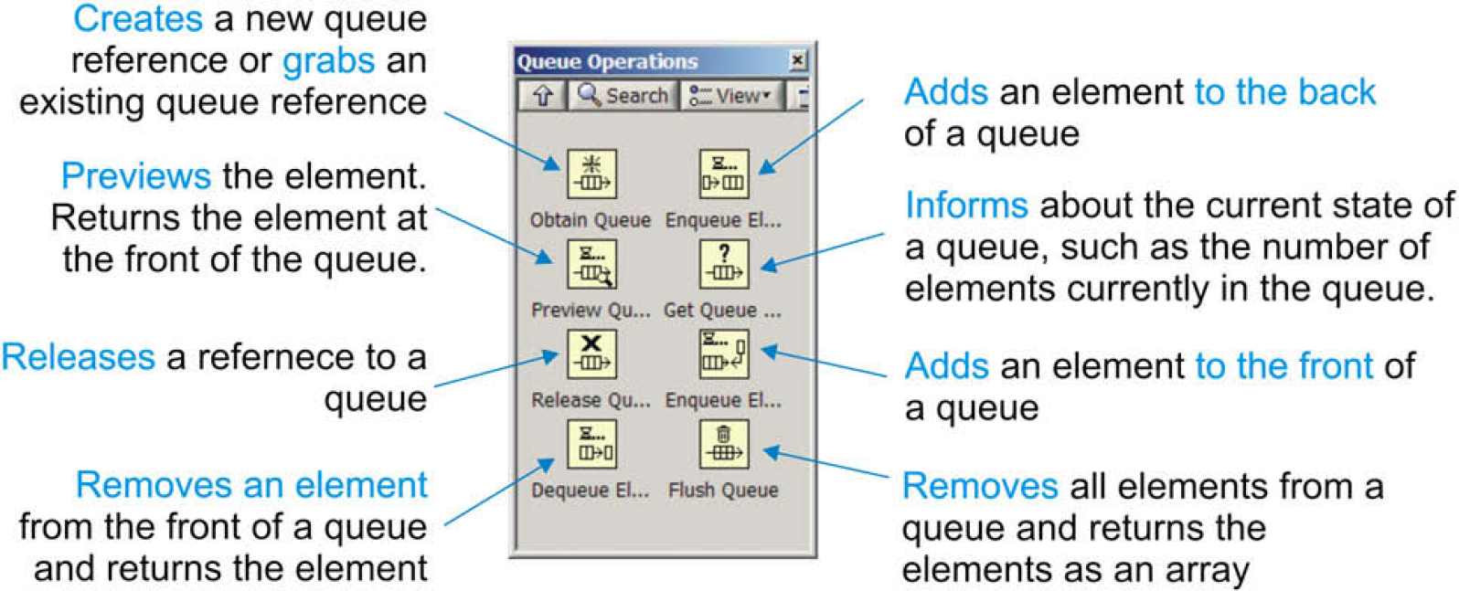
Queue palette of LabVIEW. 16
An example of simple QSM template is outlined in Figure 8. The principle of SM is preserved but other components have been added. The main advantage is the possibility to create more QSM working in parallel, independent of each other, but at the same time capable of sharing data, and if required, even controlling each other. It is even possible to dedicate each activity (particular QSM) to selected CPU core since LabVIEW 8.5, thereby improve the efficiency of the code execution (in case of multicore or multi-CPU systems).
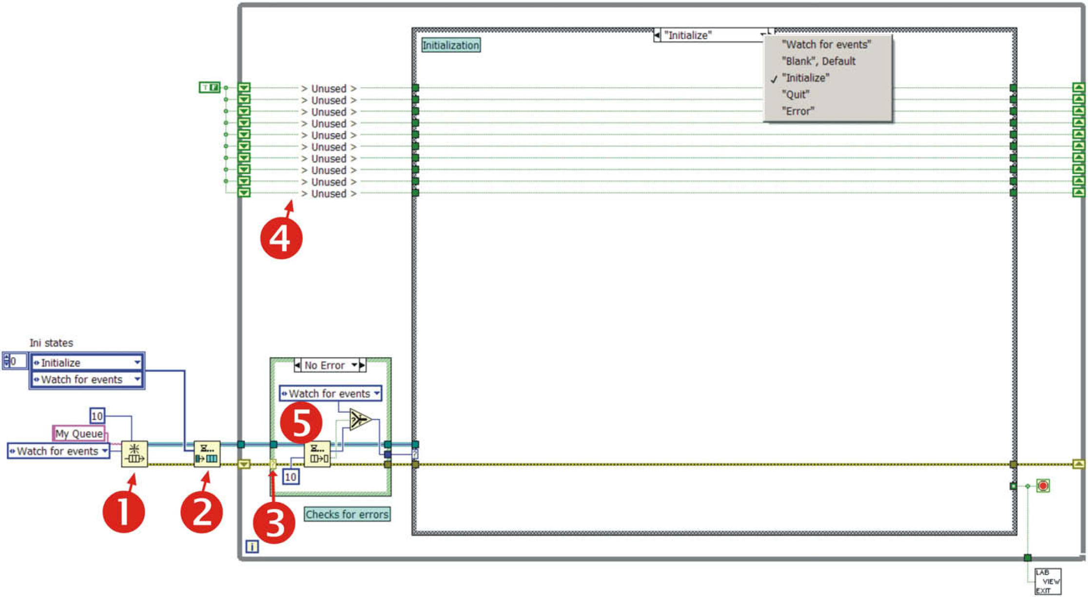
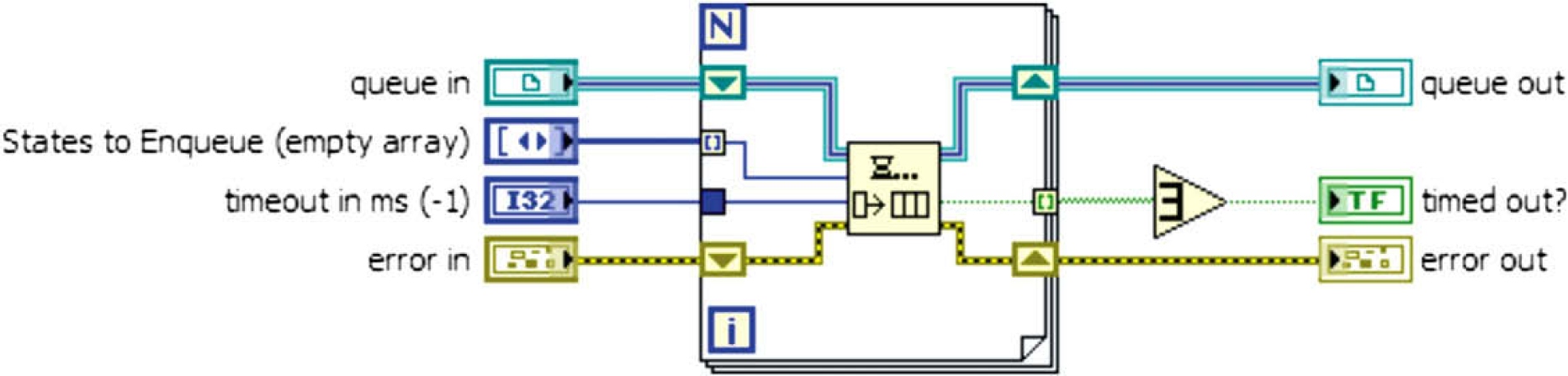
Simple QSM template.
Number 1 marks the function which creates new queue named “My Queue,” in case the queue already exists, it just grabs its reference; Number 2 ensures that all the selected states are written into the queue (for loop + enqueue element—see Fig. 9); Number 3 takes care of error checking. If an error is not detected (5), the element is removed from the queue and executed. If an error is detected, it proceeds (Fig. 10) to the “Error” state, where error handling can be performed. The application then continues; and 4 are ready-made shift registers which can store crucial variables.
Multiple state registration.
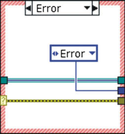
Error detection and transition to a state to handle it.
Producer—Consumer Design
During the measurement process where many time-critical operations (e.g., instruments communication) are performed, the data are acquired, and analyzed at the same time, problems with data-processing rate may appear. We measured an array of 8000 elements of double precision type (DBL) in our application which was further cut, filtered, the envelope of measured signal was computed, spectral analyses was performed, data were written into the hard-drive and after decimation, displayed in an intensity chart. They are, in general, time-consuming operations, which are repetitively manageable within 100 ms (given by the trigger interval) only with a lot of effort. So, it is necessary to find such an approach where the data output from the measurement and its repeatability is not dependent on its processing. These demands lead to the so-called Producer—Consumer design. It is based on Master—Slave pattern and is geared toward enhanced data sharing between multiple loops running at different rates. In our case, the loop that acquires data (Producer) runs faster and independent of the loop that processes the data (Consumer), which can run as fast as the remaining CPU performance allows.
OCT Application
As it was suggested in the beginning of this article, the OCT device is very complex and also the software covering it must be versatile and capable of performing tasks in parallel. It is widely recognized that multithreaded architecture poses significant programming challenges. LabVIEW offers an ideal programming environment for such a task because LabVIEW applications are inherently multithreaded.
We decided to use the techniques mentioned in previous sections to perform OCT measurements. QMSs with Producer—Consumer architecture are capable of sharing data and states between loops running in parallel. They enable parallelism of the code and the queue itself can handle simultaneous reads and writes. In addition, queues are memory efficient—they do not create any copies of the data on their own.
The three crucial operations were to assure the motion of the PZT elements, at the same time to perform DAQ and in another loop to perform data processing plus depicting of the data. In addition, transition from each scan point to another has to be done in the shortest possible time (the higher the resolution, the higher the number of points to scan and thus more time is needed). This means that processing of the data set from one scan point has to be done while the stage moves to another scan point. The benefit of the queue is obvious here. In a situation when processing of the data takes longer time than the transition to the new scan point, the device does not have to wait until the processing is done but performs the scan in parallel with data processing. New acquired data are added to the end of the data queue and are processed as soon as the loop finishes processing the previous data set. This approach saves time and, more importantly, triggers cannot be omitted. It also prevents data loss.
The application top-level flow diagram is shown in Figure 11. Solid lines represent queues where the elements are states (they are used to drive the loops) and the dashed line represents data queue. The general tasks that were mastered:
controlling of two servomotors by means of motion controller Newport ESP 300 to set the accurate position to perform each scan;
generation of a trigger signal (again using ESP 300) as a source for driving PZT elements and as a trigger signal for DAQ;
explicitly defined DAQ after trigger recognition;
data processing, depicting, and storing; and
user interface management.
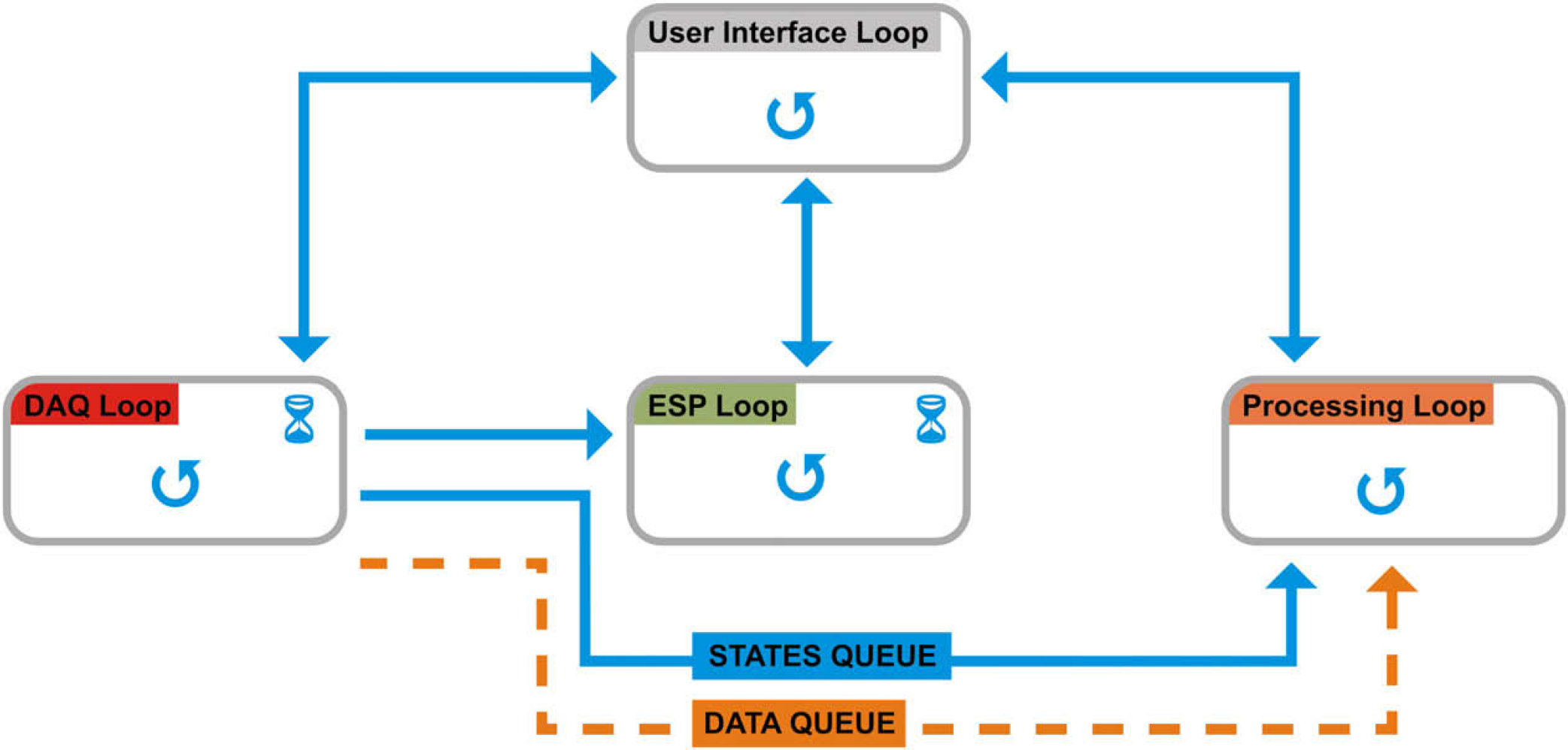
OCT application top-level flow diagram.
Description of the exact purpose of each of the loops is outlined in the following sections.
Created concept as it is described has other advantages also. Important is its modularity. It is expected that in future, some parts of the apparatus can be replaced. The program is designed so that any part of it can be altered, replaced, or upgraded without affecting the other parts and with minimum effort. This can be achieved by adding or changing states, in particular, QSM or by replacing/adding the whole QSM.
Also, if there is a need in future to deploy parts of the code to real-time hardware targets such as PXI and Compact FieldPoint, the code change will be minimal. It is even possible to run only the critical parts of the code (DAQ loop, ESP Loop) on the real-time system and the Processing Loop can be run on another PC receiving the data through the DATA QUEUE (or FIFO register). 17
User Interface Loop
The central QSM (User Interface Loop) takes care of communication with the user and on account of his demands, establishes communication with three other loops. Tasks performed by this QSM:
handles user interactions;
initializes controls and does all the maintain work before program run;
prepares datafile for writing measured data;
scales OCT image according to the dimensions of the area under examination;
establishes communication with other QSMs;
commands the DAQ loop to prepare the card circuits for the measurement; and
in case of errors, it sends commands to the other queues to safely stop them. If any error occurs in any of the loops, they immediately inform the User Interface Loop. It stops the other loops and thus the whole measurement.
DAQ Loop
The DAQ Loop takes care of the communication with the DAQ card and ensures retriggerable DAQ according to the technique described in the section DAQ. Simultaneously, it adds measured data into the data queue. Summary of tasks performed:
configuration of the DAQ card
commands the ESP Loop to prepare the ESP controller for the measurement as soon as the DAQ card configuration is ready;
communication with the DAQ card;
retriggerable DAQ;
Adds data for processing to the end of DATA QUEUE; and
checks for errors—if some errors appear, reports them to the User Interface Loop.
ESP Loop
The ESP Loop is focused on communication with the motion controller. It sets a communication port (RS232), defines velocity and acceleration of the servomotors and other essential parameters. It adjusts the start position for the stage carrying sample and after the start of the measurement, it drives the servomotors and thereby sets the exact position of the sample. It also cares about generation of the impulses for PZT-driving ramp generator and for DAQ initiation:
sets all parameters of the motion controller;
assures motion of the stage carrying the sample;
triggers DAQ and motion of the PZT elements; and
checks for errors—if some errors appear, reports them to the User Interface Loop.
Processing Loop
The Processing Loop processes the data in the DATA QUEUE. It always takes the data set from the top of the queue. The signal is filtered, the envelope of it is obtained, fast fourier transform (FFT) is calculated, and eventually, the data are decimated before picturing.
It is important to emphasize that the speed of processing is dependent only on the actual available free CPU power, so it can run as fast as possible at the moment without influencing the rates of the other loops of the application.
Processing of data from the DATA QUEUE
Checks for errors—if some errors appear, reports them to the User Interface Loop
Envelope Detection
Because the useful value of captured signal lies in its envelope, two detection algorithms were implemented. The first method consists in rectifying the signal (x 2). Squaring the signal effectively demodulates the input by using itself as the carrier wave. This means that half the energy of the signal is pushed up to higher frequencies and half is shifted toward DC. The envelope can then be extracted by keeping all the low frequencies and eliminating the high frequencies. That is reached by using lowpass (Chebyshev, third order).
The second method works by creating the analytic signal of the input by using a Hilbert transformer. An analytic signal is a complex signal, where the real part is the original signal and the imaginary part is the Hilbert transform of the original signal. The envelope of the signal can then be found by taking the absolute value of the analytic signal. Nevertheless, it is reasonable to subject the result to a lowpass filter which contributes to smoothing of the envelope.
Decimation
One of the tasks, which were necessary to handle was displaying of the measured data. Besides the graphs which depict measured signal, its envelope and frequency spectrum, an intensity chart is the main element which successively displays one B-scan by adding several A-scans (information from one point) and thus allows real-time visual control of the measurement progress. Commonly used transversal resolution is 1 μm which along with the scanned area of 500 μm x 500 μm produces 500 A-scans for each B-scan of one row. Each A-scan consists of 6000 DBLS.
The intensity chart dynamically adapts its dimensions to the dimensions of the area under examination so that the aspect ratio is preserved and the data are not biased. Let us assume that the dimensions of the chart are 350 × 800 pixels. So, we have 3.106 samples (6000 × 500) which is three orders of magnitude more than you can actually see on the graph. It causes a lot of problems which LabVIEW has to deal with. These additional operations cause slowdown when writing data into the graph and significant computing power consumption as the amount of data in the intensity chart grows. The solution is to decimate the data (of each A-scan) before displaying them.
Simple decimation methods use the first point of each decimation interval, which can lead to aliasing artifacts. The method that we used uses maximum and minimum data points of each decimation interval to provide the decimation. To minimize artifacts, at least two decimation intervals per pixel are needed. So, we take the actual height of our intensity chart and multiply it by two to get the nominal number of decimation intervals. By dividing the data length of each A-scan (6000) by the amount of decimation intervals and rounding up to the nearest integer, we get the size of the decimation interval. In each interval, Max and Min points are found and ordered as they occurred in the data set. These represent the interval after decimation. This is done for every interval. As a result of Max—Min decimation algorithm, we have four points per pixel height of the intensity chart assuring that we always see the data peaks.
Summary
The created application is fully capable of handling the OCT measurement. It was, however, necessary to use and combine advanced LabVIEW programming techniques. Final software consists of four QSMs with sophisticated producer—consumer design preventing any possible data loss and ensuring communication between all necessary instruments and broad palette of settings. The emphasis was placed on real-time evaluation of measured data, so that the scientist working with the OCT apparatus immediately knows whether the measurement runs as expected. Of course, there is lot that can be enhanced—for example, a real-time generation of topographic image would be valuable.