
Abstract
A method is presented for accurately computing the three servomechanism angles that place the leg tip of a 3DOF robot leg in cylindrical coordinate space, R, θ, Z. The method is characterized by (i) a multivariable integer power series for each degree of freedom that can be used to replace traditional trigonometrical functions, and, (ii) only integer numbers are used. A technique is shown that derives the coefficients, Ci j k, of each of the terms in the series that represents a servomechanism angle, S. This power series method has the advantage of; (i) satisfying accuracy requirements, (ii) producing a unique solution, (iii) high speed realtime computation, (iv) low memory requirement and (v) implementation into a generic algorithm or hardware such as a field programmable gate array. The series can represent many continuous kinematic systems just by changing the values of the coefficients. The coefficients are rapidly computed via a spreadsheet. The method can be extended to more than three degrees of freedom and also mapped into other coordinate frames such as a Cartesian or spherical.
Keywords
Introduction
The tabular format inverse kinematics method described in this paper originated from the programming of a six-legged robot, Fig. 1, with 3DOF legs that the author designed and built to carry out multi-agent research. Each one of the six legs is positioned in real time by one dedicated 16-bit microcomputer solving inverse kinematic equations for its designated leg. Thus six microcomputers are required for the six legs. A 7th 16-bit microcomputer sends next higher level supervisory instructions to each of the leg microcomputers. None of the seven microcomputers is capable of carrying out trigonometrical equations. Also they are not capable of working with a decimal point, i.e. only 16-bit integer calculations are allowed.

Inverse kinematics equations are developed for a six-legged robot which is shown here mounted on its calibration table
The robot is shown, Fig. 1, mounted on a calibration table which is used to set and check the positioning accuracy of the leg tip in cylindrical coordinate space. An individual cylindrical coordinate frame is used to locate each leg tip. Such a coordinate system is convenient for robot locomotion. For example, Fig. 2 and Fig. 3 show the robot walking forwards and “crabbing” sideways by programming the leg tips to follow loci that are radial paths, R, along an angle, θ, at vertical heights, Z. In fact, cylindrical coordinates enable the robot to (i) walk in any direction and (ii) turn about any instantaneous axis of rotation.

Robot walking forwards due to leg tips following loci in cylindrical coordinates.

Robot body “crabbing” sideways to the right. Actually robot can translate in any direction.
The cylindrical coordinate frame for each leg tip can be seen in Fig. 4 which shows a single 3DOF leg mounted on a calibration stand. The leg tip is calibrated along the vertical Z-axis with two aluminium blocks, (see Fig. 4). Fig. 5 shows a schematic view of the 3DOF leg kinematic system together with the leg tip located at R, θ, Z coordinates in the cylindrical coordinate frame. Note that the leg system is actuated by three integrated servomechanisms which will now be described.

A 3DOF leg mounted on a calibration stand that shows the cylindrical coordinate frame. The two aluminium blocks are 20mm and 40mm in height and are used to calibrate the leg tip along the vertical Z axis

Schematic view of 3DOF leg system showing the leg tip accessing, R, θ, Z, coordinates inside the cylindrical coordinate frame. Note that positive, Z, is downwards.
Before the inverse kinematic equations are derived and discussed it is necessary to give the reader a technical outline of the integrated servomechanisms (abbreviated to “servos”) that actuate the 3DOF leg system.
These servos are designed to follow the angular instructions that are computed by the inverse kinematic equations. The servos used for the robot are
Fig. 6 shows an overview of the integrated servo and Fig. 7 shows more details concerning the internal design of the servo.

Overview of the integrated servomechanism
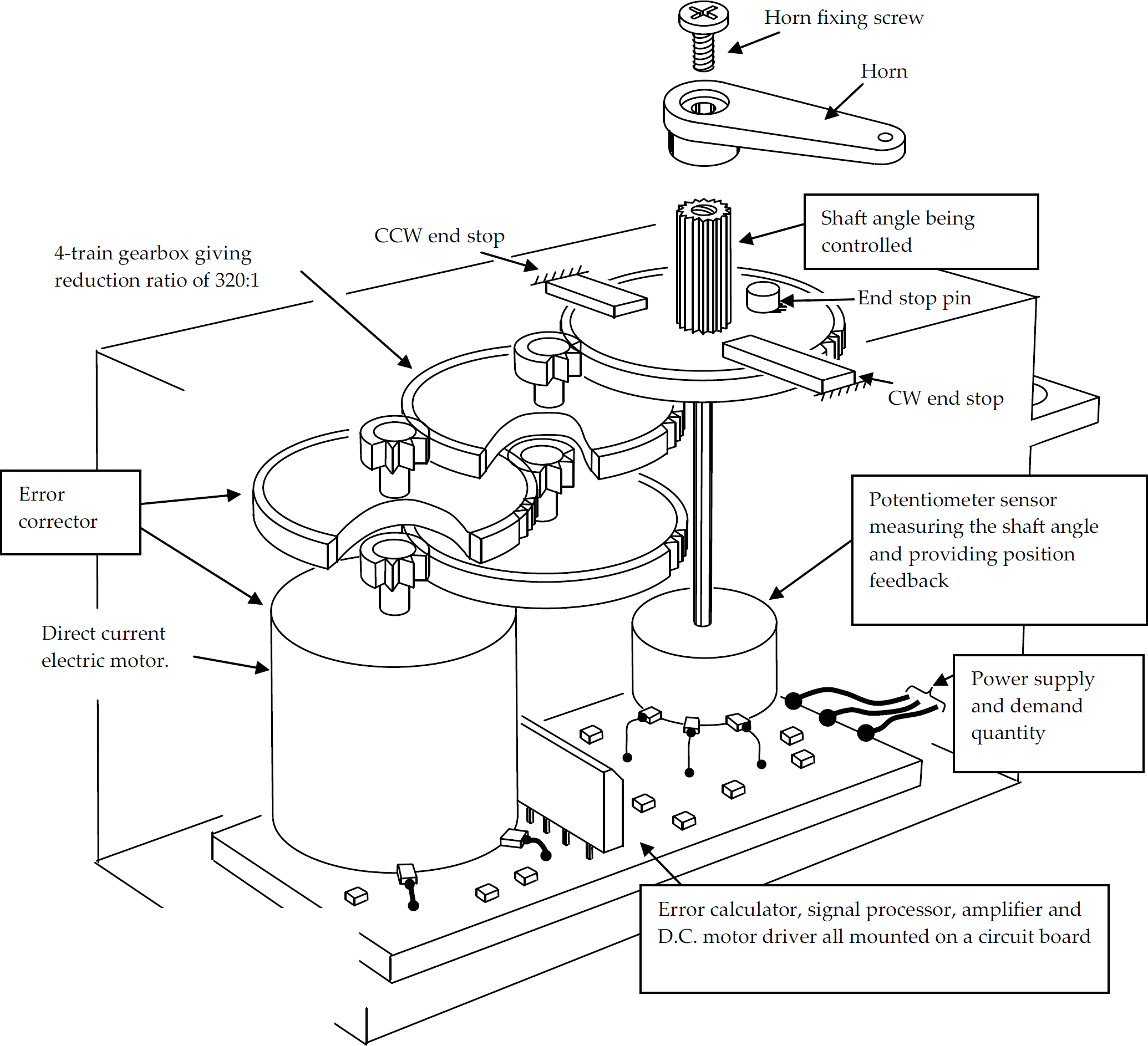
Inside the integrated servomechanism or “servo”
Integrated servomechanisms are manufactured by numerous companies, e.g. Futaba, Tonegawa Seiko, Sanyo, Ko-ProPo, HiTec. All these servos are 3-wire devices which follow the specification that wire no.1 is powered with a voltage supply of 4.8V–6V at a maximum current of 1.5A (exception is high power Tonegawa Seiko servos, 12V–24V), wire no. 2 is ground, i.e. 0V, and wire no. 3 is a pulse width modulated (PWM), 5V TTL

Pulse width modulated TTL signal representing the angle demand quantity, θ.
Fig. 9 shows the manufacturer's nominal calibration graph for the servo. The pulse width of the signal causes the output shaft to rotate to the demanded angle. The angle demand is represented by the pulse width and the period of the pulse is flexible and

Nominal calibration of servo output shaft to a demanded shaft angle, θ, with a pulse width, t, using microcomputer
It will now be assumed that we have a microcomputer with a 2 MHz clock, i.e. a clock period of 0.5μs that will be used to control each servo.
The microcomputer uses a “pulsout” instruction which produces a pulse whose length is given as follows:

These 3 lines of instruction will produce a train of pulses that is output from pin 15 (just an example). Each pulse length is 3000 × clock period = 3000 × 0.5μs = 1.5ms and the periodic time will be approximately 20ms.
Given the calibration of the Futaba servo as shown in Fig. 9, we can now derive an equation that will match the Futaba integrated servo angle, as follows:

For example, to produce a shaft output angle of +60° we require a pulsout number of 3000 + (20 × 60) = 4200. This will produce a pulse width of 4200 × 0.5μs = 2.1ms which will, in turn, cause the servo to position the output shaft to +60°. The pulsout number is an integer since the instruction counts discrete clocks pulses and cannot divide the microcomputer clock period. Hence the clock period represents the maximum resolution of the pulse width. In other words there cannot be a pulsout number with a decimal point. Half the resolution of the microcomputer clock, i.e. half a pulsout (pu) unit (=0.5μs/2), represents the lowest possible error in angle displacement of the servo (= +/− 0.05°).
In order to develop the trigonometrical inverse kinematics equations, the robot leg geometry is now considered.
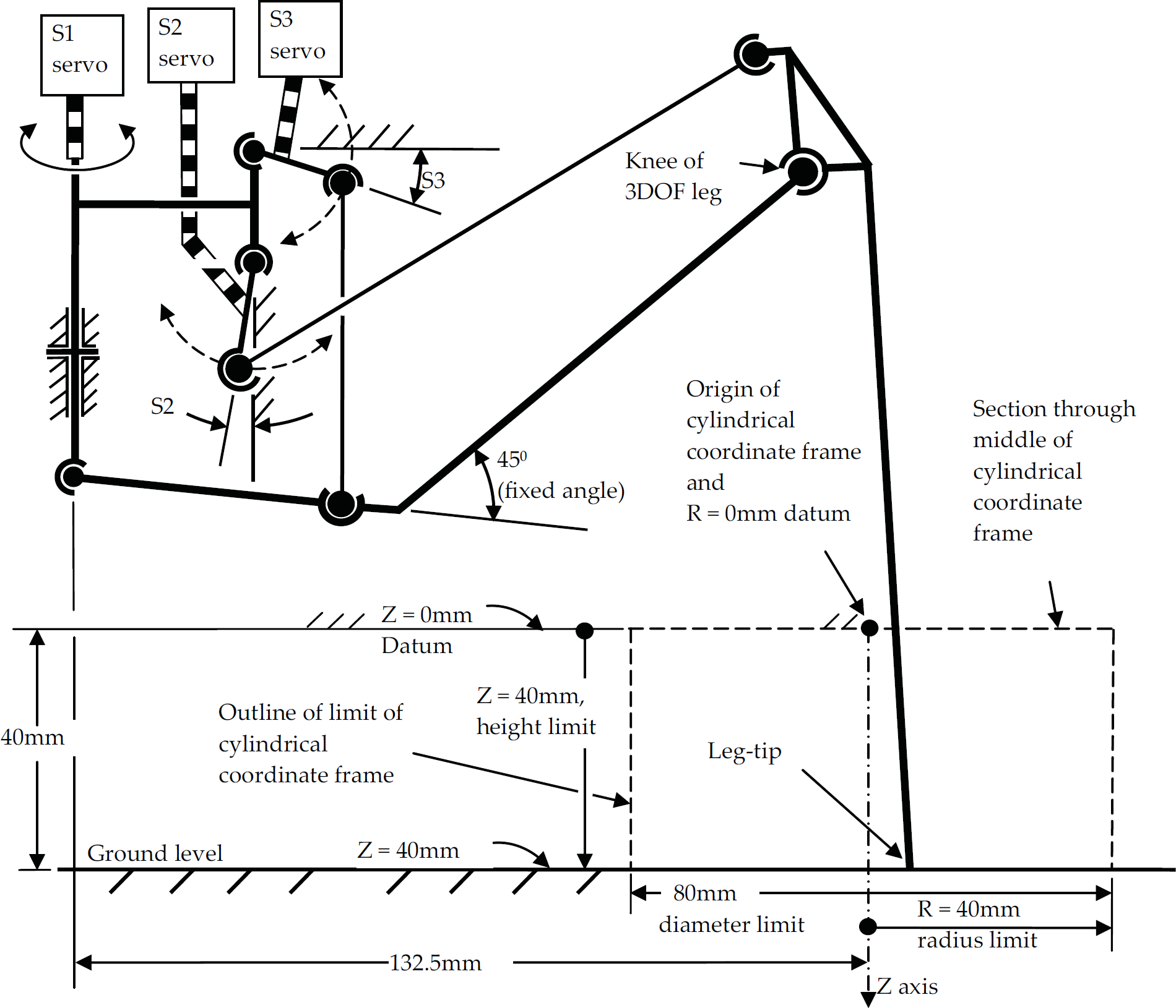
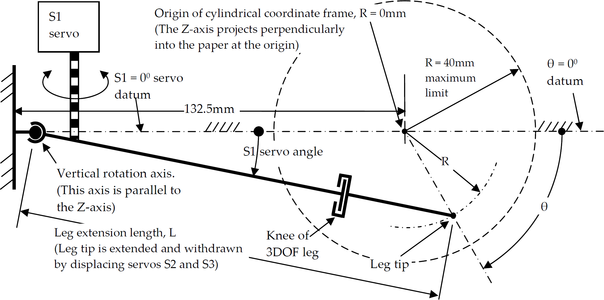
Fig. 10 shows a true view side elevation of the leg kinematics and Fig. 11 shows a plan view of the robot leg. The inverse kinematics trigonometrical equations for each of the three servomechanism angles, S1, S2, and S3 that actuate the leg tip to a location in R, θ, Z coordinates are as follows with geometrical lengths substituted in mm.
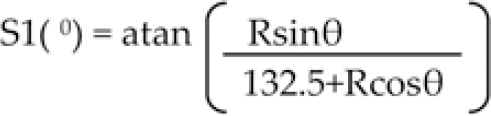
True view side elevation, of 3DOF leg system showing the three servos, S1, S2, and S3, actuating the mechanical system which place the leg tip at coordinates, R, θ, Z.
Plan view of 3DOF leg system showing the leg tip accessing the coordinates, R, and, θ, in the cylindrical coordinate frame. The S1 servo angle is independent of, Z displacement because displacement of S1 is incapable of displacing the leg tip in the Z direction which is perpendicular to the paper.
The equation, (2) above, for servomechanism angle, S1, is very straightforward and due to the mechanical design there is no function of Z in the right hand side of the equation. However the equations for S2 and S3 are much more complex and tedious to compute. The equations for angle S2 will now be presented.
Servo angle, S2, in degree units is,

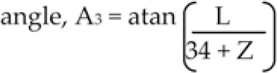
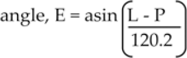
where, after substituting geometric values of the kinematic system, the values of, A2, D, and A1, are functions of R, θ, and Z, and are given by;


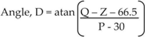
where


The The equations for servo, S3, are similar and also have a similar complexity to servo, S2. The S3 equations are not shown because the computational principles for S2 and S3 servos are the same. In order to solve these equations with a computer we require the ability to multiply, divide, add and subtract as well as to calculate sin, cos tan, asin, acos, atan and sqrt. A digital computer can only add and subtract integers of finite maximum values, e.g. 16bit, 32bit, 64bit. By using some basic software the computer can extend its ability to multiplication and division of integers. If computer programmers have need of more mathematical convenience, such as numbers with a decimal point, then more software is required to deal with these numbers. If trigonometrical functions and other functions such as log, exp, and xy, are required then even more software algorithms are needed to deal with them.
Furthermore, mathematical computers have to work to a limited number of significant figures which reflects the computational accuracy. More accuracy requires more significant figures which require more time to compute. The outcome is that computational mathematical convenience costs (i) increased memory space and (ii) increased time to execute the functions. Hence a mathematical technique, which (i) accurately imitates the trigonometrical inverse kinematics equations, and (ii) that uses integers only and (iii) has no requirement for trigonometrical or other high level mathematical functions, and (iv) reduces the number of significant figures required for accuracy, can be found then the computational efficiency should be increased. This is a fair speculation since the mathematical functions found on an electronic calculator keyboard are man-made mathematical inventions of generalized convenience anyway and that in almost all calculations, with certain exceptions, e.g. sin30°, exact results cannot be, and are not, produced. For example, electronic calculators produce accuracy to 10 significant figures and Excel spreadsheet to 15 significant figures. Indeed rarely, in engineered artifacts, is such accuracy required, Furthermore it is an essential requirement for engineering designers or researchers that a tolerance assessment is carried out in a number of forms, e.g. electronic components and mechanical component dimensioning. The same goes for mathematical computation since the cost of higher accuracy is increased computational power. The calculations shown here use the least number of significant figures in order to minimize the computational power requirements but still achieve an error not exceeding 0.5 pu (pu = pulsout unit).
The multivariable truncated power series is now introduced.
Equation (17) below will be used as a multivariable truncated power series that will accurately formulate the servo angles, S1, S2 and S3. Note that a different series is required for each servo angle.

where:
S is the pulsout integer number representing the servo angle i, j, k, are integer indices and matrix locations iT, jT, and, kT, are integers that represent the truncation indices for R, θ, and Z variables Ci j k, is the coefficient of each multivariable term in the series
To clarify eq. (17) above, as an example, let, iT =1, jT = 2, and, kT =3. Hence, S is computed like this:

It can be seen from eq.(18) that the number of coefficients, Ncoeff, required to map, S, is given by:

This number, Ncoeff, is an upper bound since if we choose to use odd or even powers or if S is independent of R, θ, or Z then the number of coefficients will be less.
Equation (17) is well known for a multivariable Taylor series (see the two references) and the coefficients can be found by taking the partial derivatives of the equation for S2. However, whereas this is not so difficult for S1, it is a difficult task for S2 and S3. The method shown in this paper is an alternative to finding the coefficients from partial derivatives.
The series, (17), forms a convenient, generic, systematic and regular computational matrix that can be used to emulate continuous inverse kinematic equations (but not at singularities) with the advantages of, (i) satisfying accuracy requirements, (ii) giving a unique solution as compared to trigonometrical equations with non-unique solutions, (iii) high speed execution suitable for realtime computation with microcomputers, (iv) relatively low memory requirement, (v) implementation into a generic algorithm or hardware such as a field programmable gate array and (vi) the method can be extended to more than three degrees of freedom and also (vii) mapped into other coordinate frames such as a Cartesian or spherical coordinate frames.
A key advantage of the series is that it can represent continuous kinematic systems just by changing the values of the coefficients, Cijk. However, there are two tricky problems to solve with the series, (eq.17), and these problems are, (i) how to calculate, the coefficients, Cijk, and (ii) how to calculate the truncated index values, iT, jT, and, kT, that give the required accuracy. Fortunately it has been found that the coefficients are rapidly computed via a spreadsheet. The procedure will now be described using servo angle, S2, as an example.
We set about finding the coefficients of the series by entering the trigonometrical equations, eq. (3) to eq. (16) into Excel spreadsheet, and then applying eq. (1) to obtain S2 in pulsout units and then plotting the relationship of S2 versus, θ, for various values of R and Z. Fig. 12 shows the resulting graphs.

Graph showing values of S2 calculated using trigonometrical equations.
Fig. 12 shows that all the relationships are symmetrical about the S2 angle axis when S2 is plotted against θ. This means we can eliminate all the odd powers of θ terms in the series. “Eliminate” in the previous sentence means to set the coefficients of the odd powers of θ to zero. Fig. 12 also shows that the graphs for, R = 40mm have the greatest curvature due to the greatest displacement range, e.g compare curves with R = 40mm to curves with R = 0mm. The latter have a curvature of zero because they are straight lines. Furthermore the curve of Z = 0mm, R = 40mm, has the greatest displacement range (=1350pu) and this implies that it is the curve with the greatest curvature. Thus the search for an integer power series should start here because such a graph with the sharpest curvature requires the greatest number of terms in a series to satisfy the +/-0.5 pulsout error band. This curve will decide what are the truncation values, iT, jT, and, kT. An integer power series designed for this worst case situation will produce lower value errors for the remaining points in the cylindrical coordinate frame.
In order to build up a 3-variable equation as shown in eq. (17), a

The equation, (20) represents the S2 angle that is required to position the leg tip along the circle shown with a blue line in Fig. 13. Note thateq. (20) has the following characteristics: (i) it possesses 8 terms, (ii) it has only even indices and (iii) the truncation index is the power of 14. The truncation index of 14 was chosen because, after experimentation with Excel spreadsheet, the eq. (20) error for computing S2 fell inside the required error of +/-0.5pu. Eq.(20) requires 8 coefficients to be derived. To do this we choose eight equi-spaced values of θ ranging from, θ = 0° to θ = 180°, on the graph of S2 versus, θ, for Z = 0mm and R =40mm. (Eight equi-spaced θ values means that the spacing is 180°/7 =25.7°). Equations (21) show the S2 values for these θ values


Leg tip describing a circle (blue line) at Z = 0mm, R = 40mm. The S2 angle is calculated as a function of θ as the leg tip describes the circle and an integer power series is derived to express this function
(Excel spreadsheet and Cramer's rule are now used to solve for the coefficients of the power series. The spreadsheet was arranged such that the θ points used to calculate the coefficients could be chosen at will and then the spreadsheet would automatically calculate a graph of error from the accurate trigonometrical equations (3) to (16). The Excel spreadsheet, simultaneously calculates the coefficients, Cijk. Errors from the trigonometrical equations are shown in Fig. 14 below where it can be seen that the errors are inside the tolerance error band at low values of θ but greatly exceed the error band at high values of θ. This is the problem of choosing equi-spaced values of θ.

S2 error graph showing the problem of choosing equi-spaced θ values when using Cramer's rule to solve for the coefficients of the integer power series equation. The problem is that the S2 errors are well below the tolerance of +/-0.5 pulsout units near the origin of the graph but wildly greater than the tolerance at greater values of θ. The error, however, does reduce to zero at θ = 180°.
This unbalance of the errors can be rectified by a nonlinear shift of the coordinates used to calculate the coefficients. By using a new set of θ coordinates, spaced non-linearly, eqs. (22), an acceptable set of errors is produced without increasing the truncation index values.
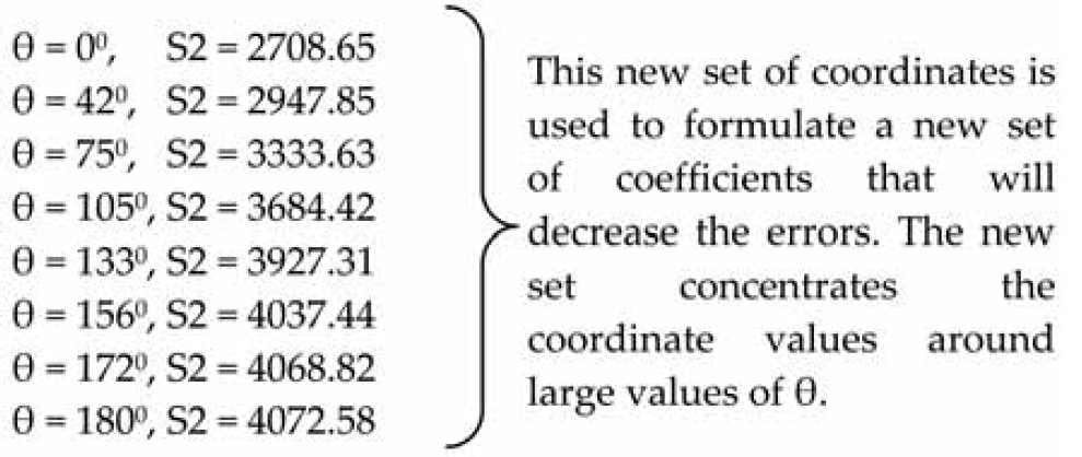
The strength of the spreadsheet is that it allows the operator to play at will with a new set of θ values which gives an immediate feedback of the effect on the errors. (However it would be better to have an equation which sets the values of θ by a systematic method). Keeping the errors inside the tolerance error band is like keeping a long vigorously wiggly snake down on the ground with eight sticks and takes time to work out values of θ.
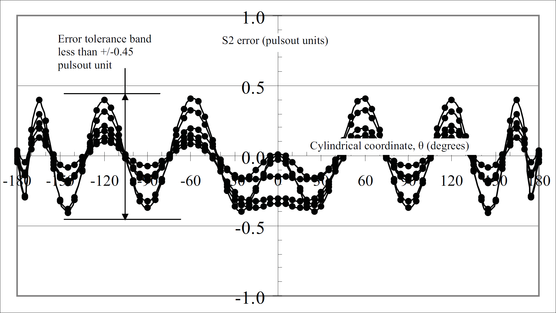
The body of the “snake” is more vigorous the further is θ away from 0°. Fig. 15 shows the errors, with the new set of coefficients. It can be seen that the errors oscillate between approximately constant tolerance limits of +/-0.4 pulsout unit which is acceptable since is less than the target +/-0.5 pulsout unit.

Errors in the calculation of S2. The eight values of θ, which are chosen to solve for the eight coefficients are chosen carefully to give near constant maximum errors which are in this case +/-0.4 pulsout units.
The equation based on eq. (20) that produces the acceptable errors shown in Fig. 15 is given with the following coefficients, eqs.(23).

And to make things very clear we use these coefficients, (eqs. 23), to write down the equation, (24), which represents S2 at R = 40mm in the Z = 0 mm plane.

For illustration purposes the coefficients in eq. (24) have been truncated to 3 sig. figs. for convenience. Readers are reminded that all calculations are done with the full complement of 15 sig. figs. supplied by Excel spreadsheet. As soon as the final equations have been worked out then the sig. figs. can be truncated to give an acceptable accuracy.
It is also necessary to note that, except for rare cases such as sin30°, there is rarely the phenomenon of exact computation performed by calculating devices. Rather, that calculating devices are designed to give accuracy to a certain number of significant figures which decides the accuracy of calculation.
The next step is to use Excel spreadsheet to calculate more sets of coefficients in the Z = 0mm plane at various values of radius, R. Suitable circles are at radii, R = 0mm, 20mm, and 30mm and then the process is repeated for circles at the same radii at Z = 10mm, 20mm 30mm and 40mm. These circles are clarified in Fig. 16 below which shows 25 circles made up from five Z planes and five R cylinders, (including R = 0mm). For each circle the coefficients for each term in the eight-term integer series are worked out by the spreadsheet. One graph is allocated for each of the eight coefficients. On each graph there are 25 coefficients derived from each of the 25 circles. The Excel spreadsheet is ‘magically’ quick in working out all the coefficients for each of these values and then turning them into graphs. The following eight graphs show how the coefficients, CR0Z, CR2Z, CR4Z, CR6Z, CR8Z, CR10Z, CR12Z, and CR14Z, vary with R and Z.
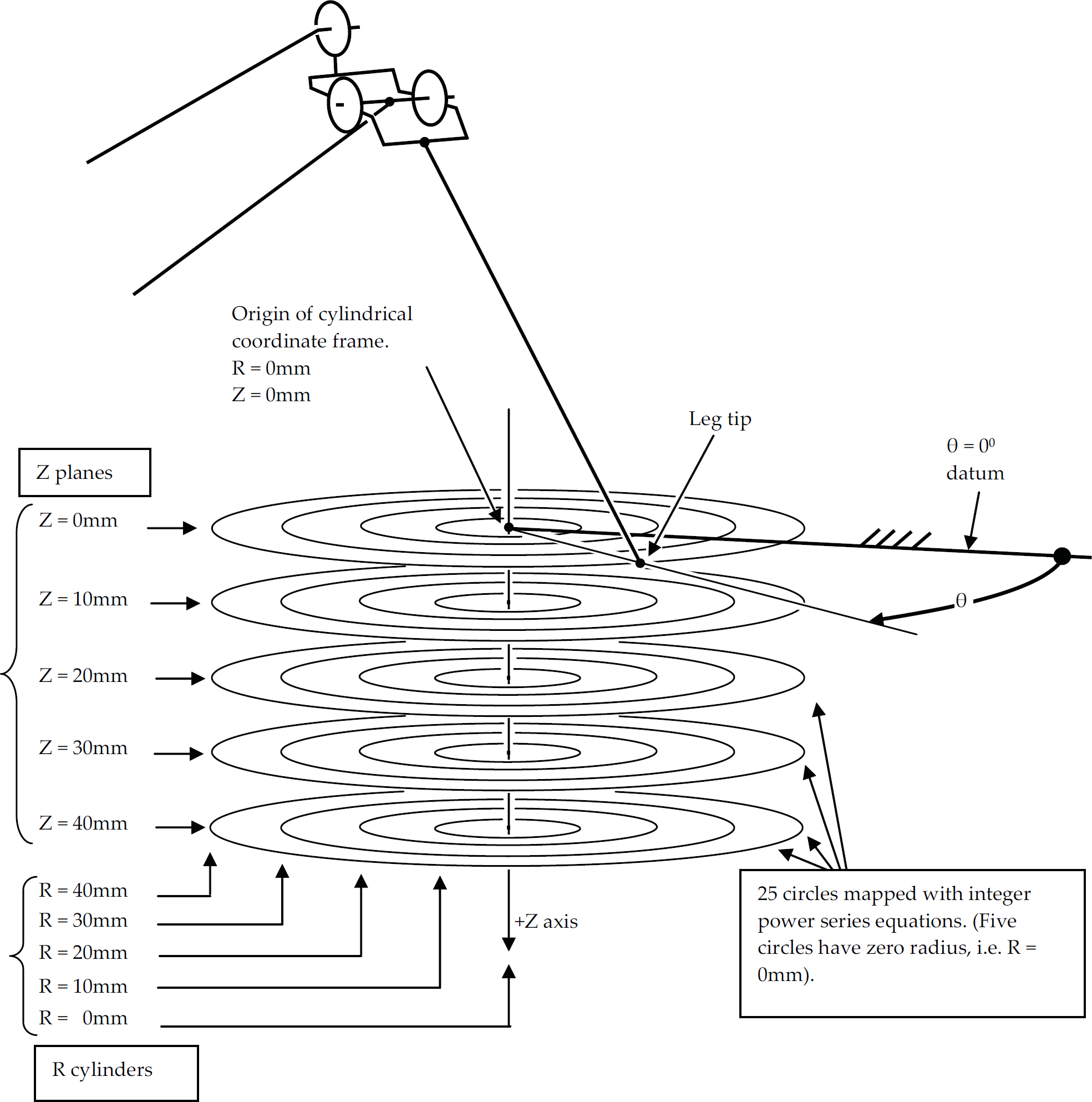
Diagram showing the circles that are mapped by integer power series equations whose coefficients are shown in the following eight graphs

Variation of coefficient, CR0Z, for various values of R and Z
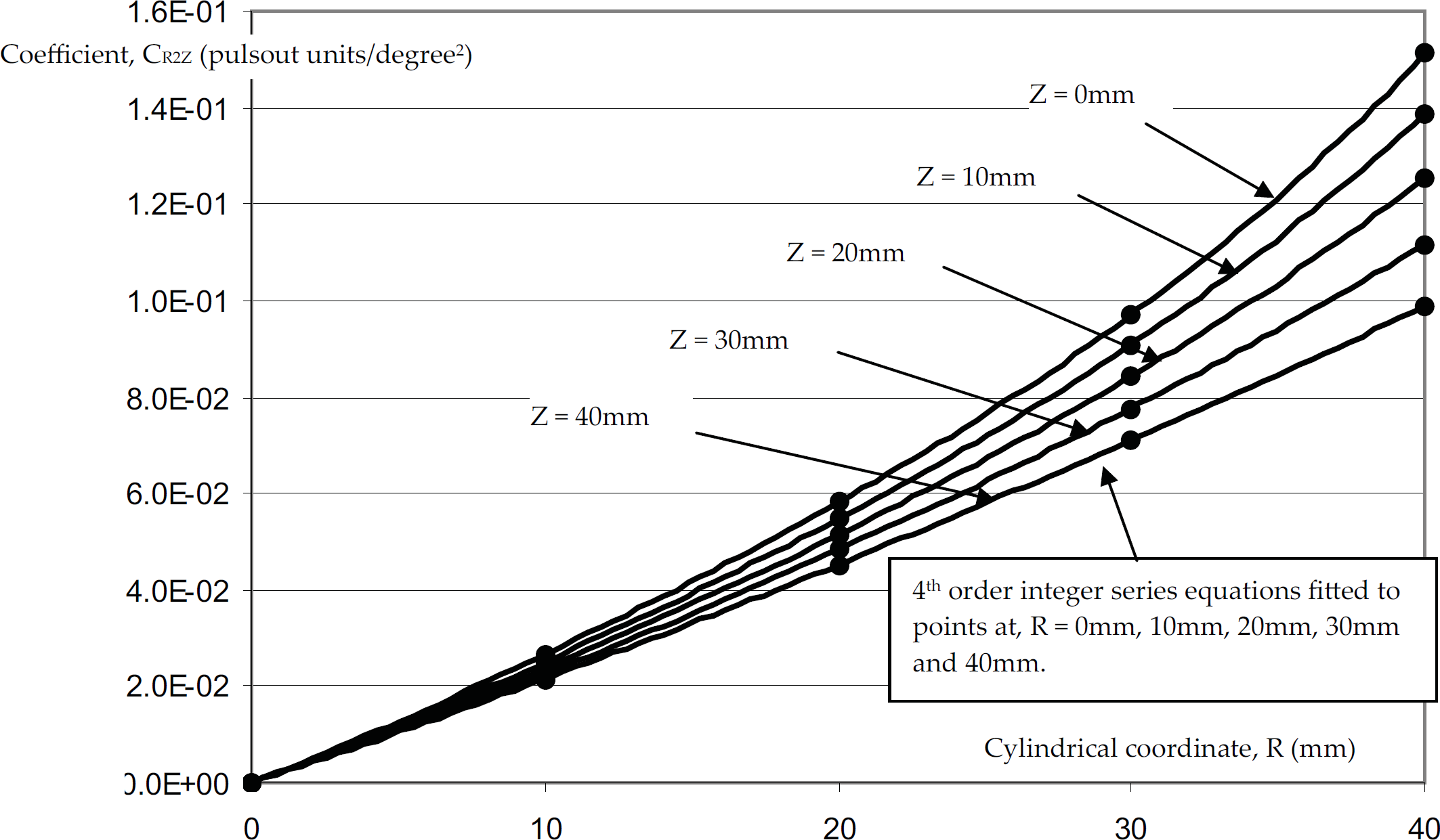
Variation of coefficient, CR2Z, for various values of R and Z
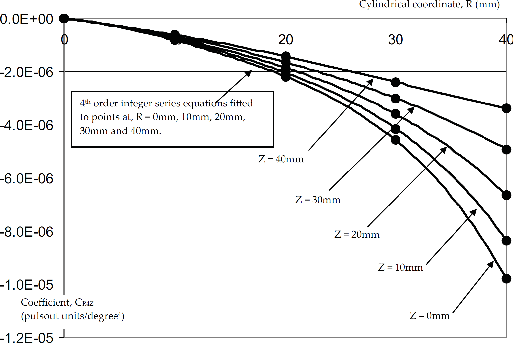
Variation of coefficient, CR4Z, for various values of R and Z

Variation of coefficient, CR6Z, for various values of R and Z

Variation of coefficient, CR8Z, for various values of R and Z
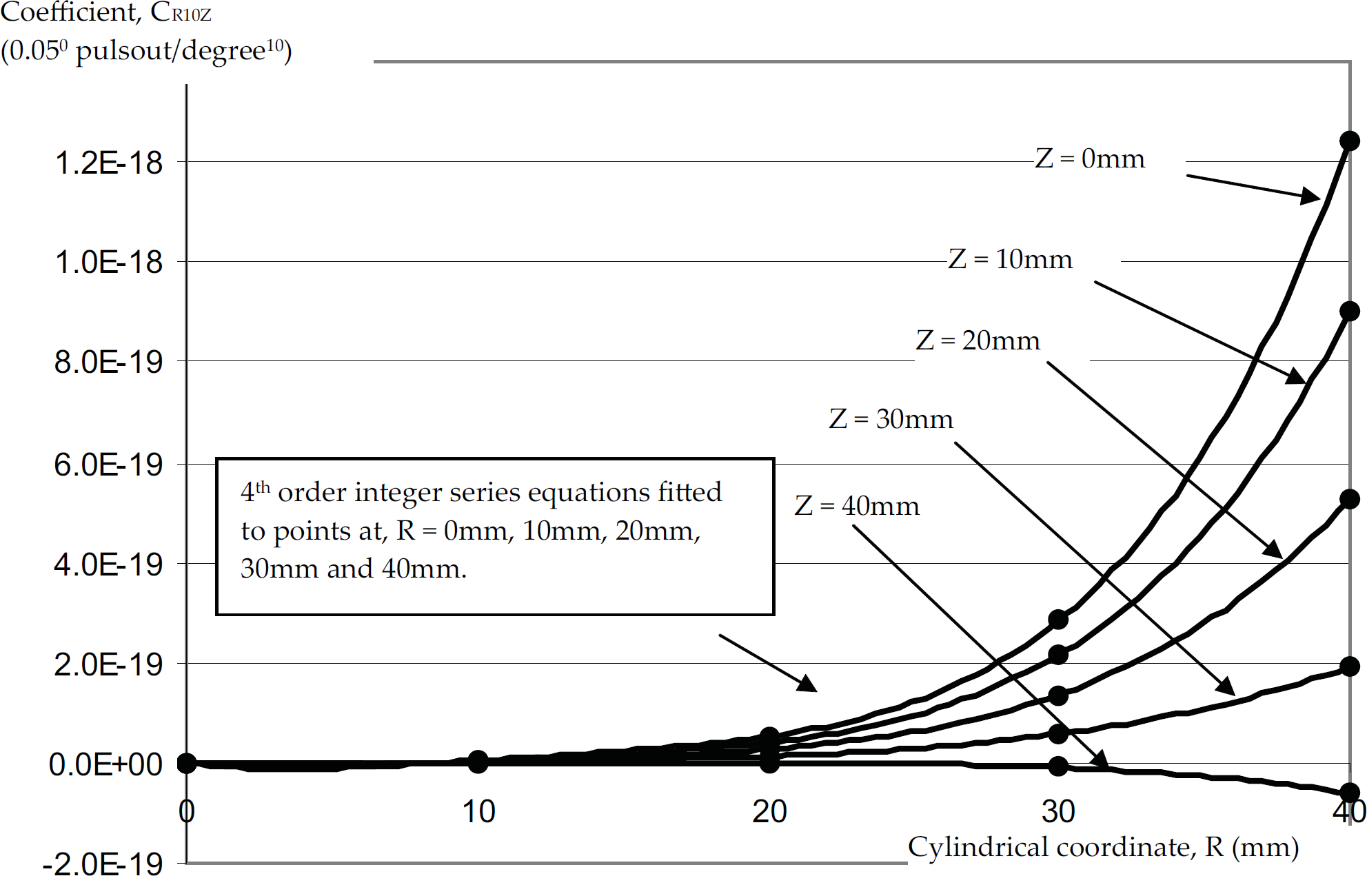
Variation of coefficient, CR10Z, for various values of R and Z

Variation of coefficient CR12Z for various values of R and Z
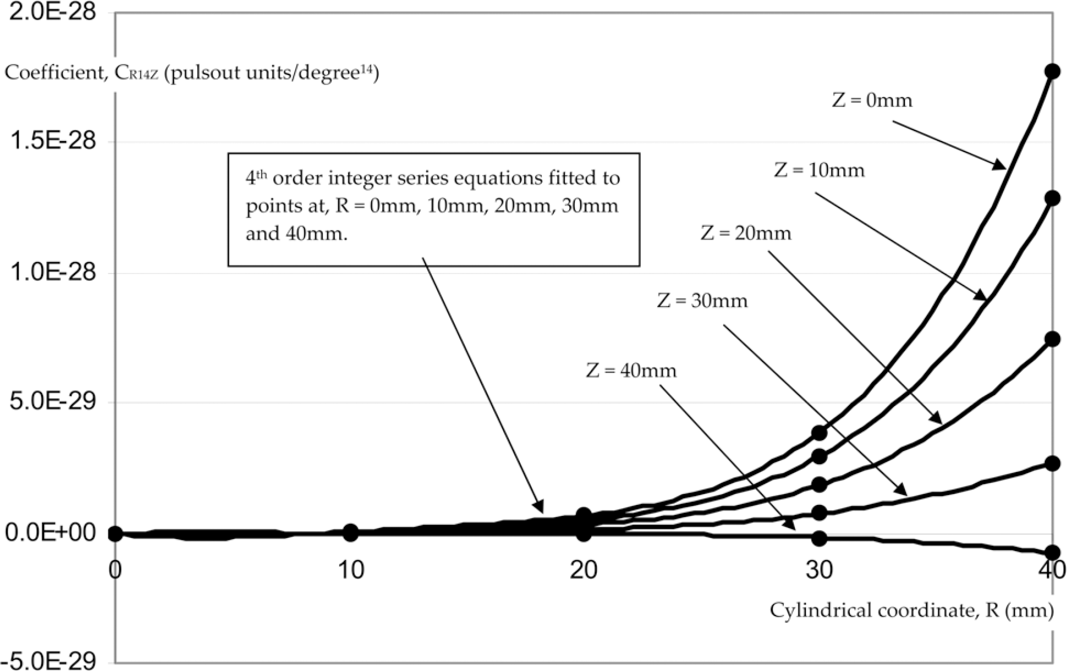
Variation of coefficient CR14Z for various values of R and Z
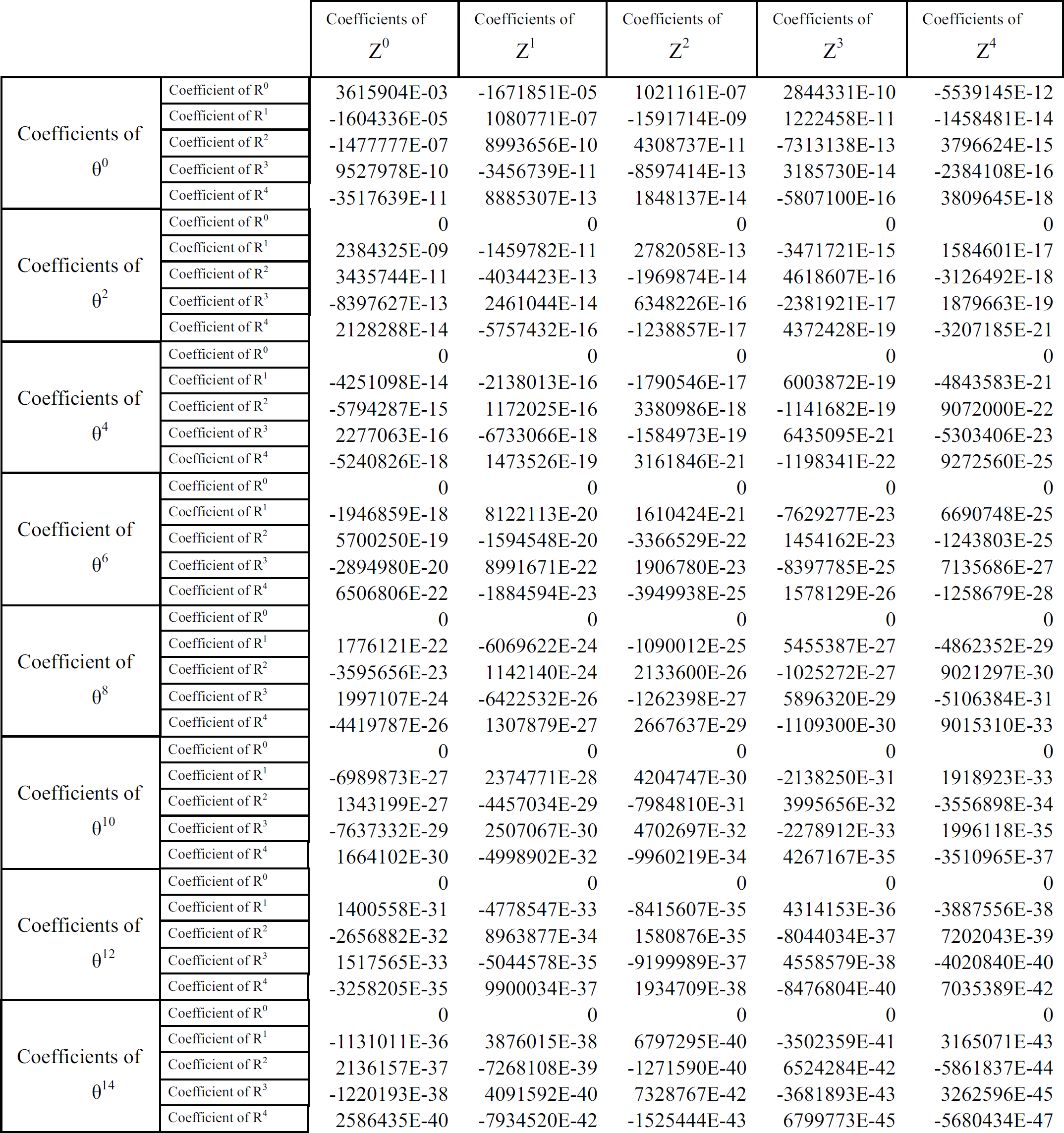
Fig. 25 below shows a table, which lists all the coefficients of θ for the values of R and Z that have been plotted in the preceding eight graphs. The next step in the computation data compression of S2 is to take the coefficients in Fig. 25 and to map the coefficients as a continuous 4th order integer power series equation as a function of R. Hence we are deriving coefficients of a new set of equations that maps each of the five discrete Z planes, Fig. 16, i.e. at Z = 0mm, 10mm, 20mm, 30mm and 40mm.

Table of coefficients, extracted from the preceding eight graphs, for the initial data compression of the computation of S2. Note that the values have been computed with Excel spreadsheet, which stores the values as 15 significant figure numbers but the table shows the values with much reduced number of significant figures just for convenience. More significant figures will be required for the final equation to obtain the required accuracy.
Why 4th order? Well, this is considered of sufficient order to give a final error of S2 that satisfies the error band tolerance of +/-0.5 pulsout unit but these errors will be checked later. This seems unscientific but the method in this paper still requires improvement. A 4th order equation requires five points to solve for the five coefficients. These points are at R = 0mm, 10mm, 20mm, 30mm and 40mm, as shown in Fig. 25 below. Fig. 26, below gives an example of how the set of coefficients, CR0Z, is mapped into each of the five Z planes.

Below are shown five 4th order equations of the coefficients, CR0Z, at five different Z planes. Note that, once again, the number of significant figures of the coefficients has been truncated in order to get across the principle of the operation.
The above five equations, (26) to (30), can be used to compute the θ° coefficient for any point R, θ, Z, in the cylindrical coordinate frame volume.
The above example operation in deriving coefficients is carried out on the remaining data of Fig. 25. This action produces a new set of coefficients listed in Fig. 27 and then a final set of coefficients listed in Fig. 28.

Table of coefficients, shown to 3 sig. figs. for convenience, of continuous integer power series equation for computing S2. Note that there are 200 coefficients that represent 40 continuous equations in five different Z planes that can compute S2 as a function of R and θ. However, the coefficients do not represent continuous equations as a function of Z. The next step is to make continuous equations for S2 as a function of R, θ and Z.
This is it These are all the data you need to compute the value of S2 for all values of R, θ and Z that lie inside the cylindrical working volume of the leg tip. The table lists all the coefficients that will compute S2 from a 3-variable integer power series that is based on R, θ, and Z. Note that there are 200 coefficients but, of these, 35 are zero. The coefficients are shown accurate to 7 significant figures which give satisfactory accuracy. (See figures 29 and 30).
All the operations that derive coefficients of integer power series equations use the Excel spreadsheet and Cramer's rule. The Excel spreadsheet trendline polynomial fit is not used because this does not allow the automatic loading of coefficients into cells for the next step of calculations.
It needs to be said that the really useful property of the Excel spreadsheet is that you can handle so many numbers in an orderly manner and this is vital when there are so many equations and coefficients to manipulate. In fact one can go as far as saying the multivariable integer power series technique has been made possible by such a computer-aided product.
It is necessary to make clear how all the coefficients in the Fig. 28 are used to compute S2. Hence the equation for the computation of S2 is shown below, eq. (31), but due to space constraints, showing the coefficients truncated to 3 sig figs and only the first two coefficients of θ, i.e. coefficient of θ° and coefficient of θ2, and the last coefficient of θ, i.e. coefficient of θ14.
Fig. 29 shows a sample of the maximum errors of the integer power series compared to the ‘true’ 15 sig. fig. Excel spreadsheet trigonometrical equations. It can be seen that the maximum value of errors are less than +/−0.45 pulsout unit and thus do not exceed the specified tolerance of +/−0.5 pulsout unit. A multivariable integer power series with such an error tolerance band is considered accurate.
Sample of maximum errors for the computation of S2 using an integer power series and 7-sig fig coefficients. Maximum errors are incurred at low values of Z, (Z = 0, 5, 10mm) and high values of R (R = 40, 35, 30mm). This information found using Excel spreadsheet
The next step is to truncate the 15 sig. fig Excel spreadsheet coefficients to a minimum number that still maintains the specified error tolerance of +/−0.5 pulsout unit. The idea is to economise on the computational effort. It is a waste of resources to compute equations to an unnecessary low error. It is found that 6 sig fig coefficients exceed the error tolerance but 7 sig fig coefficients add only an extra error of +0.05 pulsout unit and this error occurs at high values of R, θ and Z. This error can be seen in Fig. 30. Combining the errors of fig 29 and 30 produces an error not exceeding the specification of +/−0.5 pulsout unit. Hence 7 sig. fig. coefficients are deemed sufficiently accurate.

Error between integer power series with 7-significant-figure coefficients and integer power series with 15 significant figure coefficients. Error shown is the worst case which is computed at R = 40mm and Z = 40mm.
A similar technique is applied to the development of the S3 and S1 series and the results are shown in Fig. 31 and equation (32) respectively. Note that the equations for S2


This is it!. This is how S3 is computed. The table lists all the coefficients in six-figure format for the 3-variable, R, θ, Z, integer power series computation of S3.
and S3 contain only even powers of θ but the equation for S1 contains only odd powers of θ. Also note that the coefficients for S1 and S3 are only required to an accuracy of 6-sig figs to give the required error of less than +/-0.5 pulsout units.
A technique has been shown that develops the coefficients of a 2 and 3-variable integer power series that accurately fits complex inverse trigonometrical equations. One multivariable integer power series is required for each degree of freedom. The equation for each degree of freedom has different coefficients. The technique is general in that it can be used for many kinematic systems
Future work
Future work is required to measure the computation execution times on a digital computer that compare the times of execution between the multivariable integer power series and the traditional inverse trigonometrical equations. The technique should be computed on a field programmable gate array and computation execution times measured. The realtime execution time and memory requirement has not yet been proven to be less in both cases than solutions carried out with traditional trigonometrical inverse kinematics. The Excel spreadsheet method for finding the coefficients for the series is, at present, manually interventional to produce errors that do not exceed a given value. (Note that the method is not a least squares error fit). Work is required to automate this process, i.e. to decide automatically the truncation index values and also the zero crossing points. A method should be devised whereby the series coefficients are learnt by an on-board technique that derives coefficients by another series but the learnt series should have fixed, “born with”, coefficients.
