Sage Journals: Discover world-class research

Abstract

This article presents an analysis of computational efficiency to solve the inverse kinematics problem of anthropomorphic robots. Two approaches are investigated: the first approach uses Paul’s method applied to the matrix obtained by the Denavit–Hartenberg algorithm and the second approach uses Gröbner bases theory. With each approach, the problem of inverse kinematics for an anthropomorphic robot will be solved. When comparing each method, this article will demonstrate that the method using Gröbner bases theory is more computationally efficient.

Keywords

Robotics anthropomorphic robots inverse kinematics computational efficiency Paul’s method Gröbner bases theory

Introduction

Two classic problems in the kinematics of robotic manipulators are forward kinematics (FK) and inverse kinematics (IK). In FK, the position and orientation of the end-effector are calculated from the joint variables. In the IK, the movements of individual joints are calculated from the position and orientation of the end-effector of a robotic manipulator.

According to Daya et al.,¹ one of the biggest problems in kinematics and robot control lies in determining the solution of IK. Still, according to the same authors, as the complexity of the robotic manipulator increases, obtaining the IK is difficult and computationally expensive. Traditional methods, such as geometric, iterative, and algebraic, are inadequate as the geometric structure of the manipulator becomes more complicated.

Paul et al.² used matrix algebra to obtain a solution to the IK problem of a specific manipulator robot. Lee³ and Yih and Youm⁴ used a geometric approach to solve this problem. Subsequently, Huang and Milenkovic⁵ and Manseur and Doty⁶ developed iterative procedures to solve the IK problem.

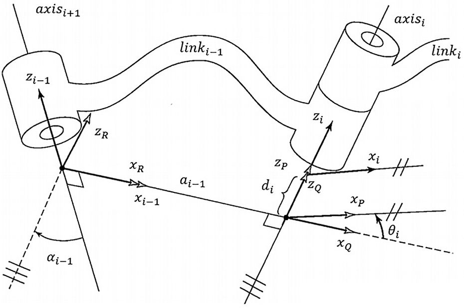
Denavit and Hartenberg⁷ introduced a convention to standardize the reference coordinate systems for spatial links; after a decade, the same authors presented an algorithm for solving the kinematics problems of articulated systems.⁸ The importance of this algorithm for the kinematics analysis of robotic systems was studied by Paul⁹ 16 years ago.

An alternative method for the solution of IK will be used in this article, namely the Gröbner bases theory. The computational performance data obtained in this article will prove that this choice will reduce the computational cost for the solution of the IK problem of serial robotic manipulators compared to Paul’s method.

The Gröbner bases theory, developed by Bruno Buchberger in his PhD thesis, consists of an algebraic algorithm that can be applied to a given set of nonzero polynomials, producing a finite set of generators, so that it is possible to identify from these generators when a specific polynomial belongs to the original given set.¹⁰ When finding solutions for this set of generators, those are also solutions for the whole set. With the aid of MAPLE, an algebraic computing software, all these solutions can be calculated, including cases not so easily solved using matrix algebra or geometric applications due to the complexity of the geometry of some manipulator robots.

Kendricks,¹¹ in her PhD thesis, compared the algorithm of Denavit and Hartenberg with Gröbner bases theory for the solution of the IK problem. Her analysis focused on the robot Fanuc A-510, a SCARA type robot, with three degrees of freedom.

To familiarize the reader with each method, the anthropomorphic robot Unimation PUMA 560, a manipulator with six rotary joints, will be used as a case study applying Paul’s method from the Denavit–Hartenberg matrix and the method proposed in this work to solve the IK problem. The main goal of this article is to analyze the computational efficiency in solving the problem of the IK of anthropomorphic robots using both methods.

Guzmán-Giménez et al.¹² presented a systematic procedure for the solution of IK problem of nonredundant open-chain robotic systems using Gröbner bases theory after solving the FK from the Denavit–Hartenberg algorithm; however, it is worth mentioning that the authors restricted themselves to the first three joints of the anthropomorphic robot Unimation PUMA 560.

Ni and Wu¹³ presented an algorithm to solve the IK of a generic 6R robot based on matrix employing quaternions as spatial operators and the Gröbner bases theory. Through the algorithm presented by the authors, 16 different solutions are determined, but, among these, only four solutions are real. As this method is not compared to any other, its computational efficiency could not be confirmed.

Unlike Wang et al.,¹⁴ who also presented a solution for the IK of a 6R serial manipulator using Gröbner bases theory, a base with a reduced number of polynomials will be determined in this article, since these authors, using the solution method of the kinematics of mechanisms proposed by Duffy and Crane,¹⁵ produced a Gröbner basis with 72 polynomials. With a reduced number of polynomials, which will be presented in this article, this base will increase the computational efficiency of the calculations to obtain all the joint configurations.

El-Sherbiny et al.¹⁶ presented a comparative study between different soft-computing-based methods (artificial neural network, adaptive neuro-fuzzy inference system, and genetic algorithms) applied to the problem of IK. Their analysis focused on a serial manipulator with five degrees of freedom, and the results of the analysis demonstrate that the methods are not accurate and computationally efficient at the same time. The choice of method depends on the application, being necessary to decide which one has more priority, the calculation time or the accuracy.

However, the present work intends to go further. It brings an analysis of the computational efficiency in the solution of the IK problem of a serial manipulator with six degrees of freedom using Gröbner bases theory. The obtained results will be compared with those obtained by Paul’s method from the matrix obtained by the Denavit–Hartenberg algorithm, demonstrating that the Gröbner bases theory method is more computationally efficient and that the solutions obtained from this method are accurate.

Gröbner bases theory

The core of Gröbner bases theory is an algorithm used to solve systems of polynomial equations. It is known as Buchberger’s algorithm and applies computational algebra techniques to polynomial ideals, producing a so-called Gröbner basis, a new polynomial set.

Briefly, a Gröbner basis for a polynomial equation system is a new collection of polynomials in which the null set coincides with the solution set of the original system; however, this new system is simpler to solve. This definition justifies the choice of Gröbner bases theory to solve the IK of serial manipulators with the reduction of computational cost.

Gröbner bases theory is widely applied in other areas besides mathematics. For example, Cox et al.¹⁷ have dedicated their work to the applications of Gröbner bases theory in geometry, graph theory, and robotics.

According to Sturmfels,¹⁸ a Gröbner basis can be computed in order that the polynomials have a property known as the elimination property. This elimination property makes the computation of solutions of a polynomial system, which is a Gröbner basis to be mathematically efficient because, through retroactive substitutions, a solution can be found for the remaining set of variables, with a reduction in the number of floating-point operations.

For polynomials with several variables, the complexity for the determination of a Gröbner basis depends not only on the number of polynomials in the set but also on how their terms are ordered. The lexicographic order is particularly suitable for solving systems of polynomial equations. In a lexicographic order, a variable dominates any monomial involving only minor variables, regardless of the total degree. For example, for the lexicographic order $x ≻ y ≻ z$ , thus $x^{2} ≻_{l e x} y^{12} z^{8}$ .

It can be seen in Figure 1 that all variables can be solved consecutively because the obtained Gröbner basis is a triangular equation system.

Figure 1.

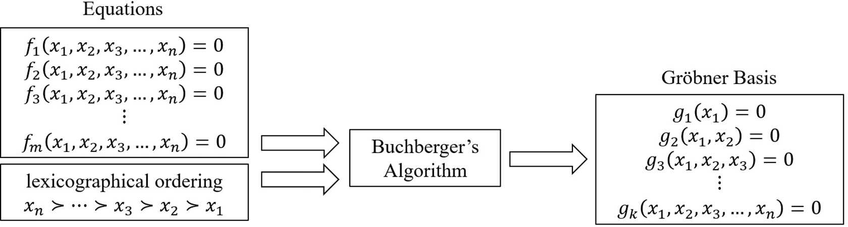
Input and output of Buchberger’s algorithm.

In some cases, one chooses to consider the total degree of a monomial and to order the monomials of larger degrees first. In this specific case, the graduated lexicographical order (grlex) is used. Another order is given by the reverse graduated lexicographic order (grevlex), which is commonly used because it generally provides the basis more quickly due to a reduction in computational cost.

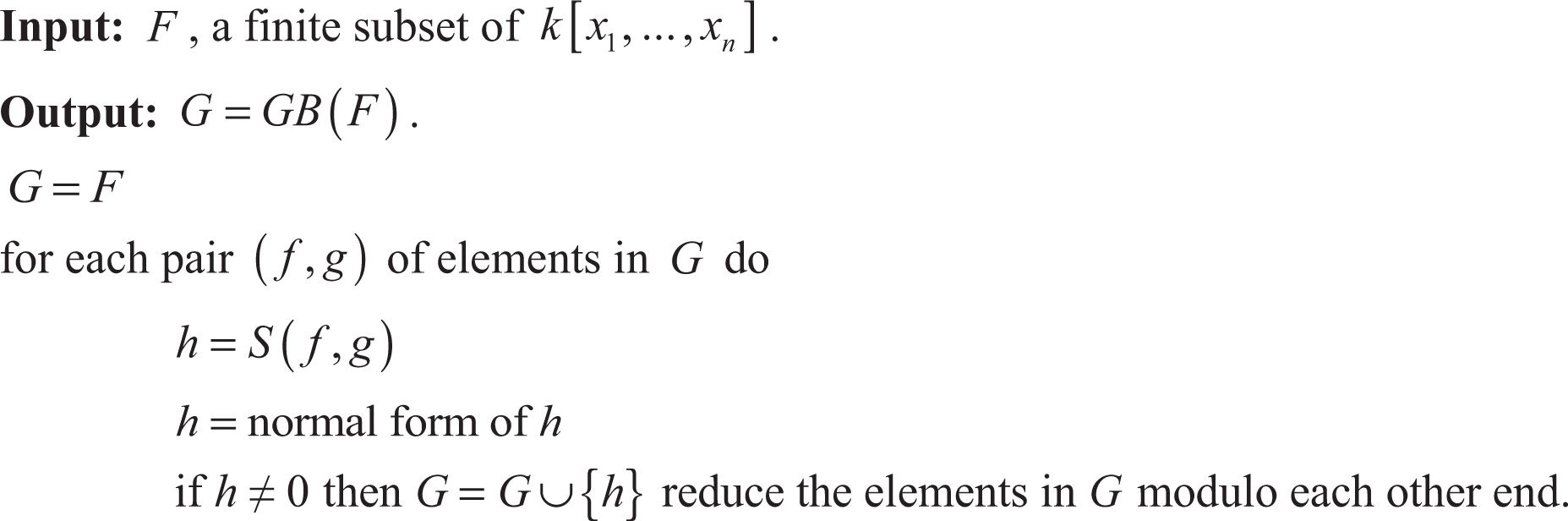
Buchberger’s algorithm constructs a Gröbner basis starting from a finite set of polynomials. According to Cox et al.,¹⁷ to develop Buchberger’s algorithm, it is necessary to understand the nature of S-polynomials.

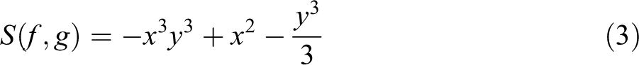
Let f and g be two nonzero polynomials and consider $L = lcm (lp (f), lp (g))$ , where lcm is the least common multiple among the leading power products $(lp)$ of polynomials. The combination $S (f, g) = \frac{L}{lt (f)} f - \frac{L}{lt (g)} g$ is called the S-polynomial of f and g, where (lt) stands for the leading term of each polynomial.

As an example, $f = x^{3} y^{2} - x^{2} y^{3} + x$ , $g = 3 x^{4} y + y^{2} \in ℝ [x, y]$ , with lexicographical order $x ≻ y$ , it is intended to determine: $S (f, g)$ . To solve this problem, it is necessary to determine $L = lcm (lp (f), lp (g)) = lcm (x^{3} y^{2}, x^{4} y^{2})$ . Thus

S (f, g) = \frac{x^{4} y^{2}}{x^{3} y^{2}} f - \frac{x^{4} y^{2}}{3 x^{4} y} g

S (f, g) = x (x^{3} y^{2} - x^{2} y^{3} + x) - \frac{y}{3} (3 x^{4} y + y^{2})

S (f, g) = - x^{3} y^{3} + x^{2} - \frac{y^{3}}{3}

Note that the S-polynomial is produced to cancel the leading terms of the polynomials involved. The Buchberger’s algorithm receives as input a finite set $F = \{f_{1}, f_{2}, \dots, f_{n}\}$ of polynomials and provides a set G, which is a Gröbner basis of $F .$ According to Stifter,¹⁹ this algorithm can be described as follows.

Algorithm 1.

Algorithm for computing Gröbner bases.

Faugère²⁰ presented an efficient algorithm for computing Gröbner bases: the F4 algorithm. This algorithm computes successive truncated Gröbner bases, and it replaces the classical polynomial reduction found in the Buchberger’s algorithm by the simultaneous reduction of several polynomials. This powerful reduction mechanism utilizes symbolic precomputation and sparse linear algebra methods.

With the help of algebraic computing software, a Gröbner basis can be calculated more quickly. Many algebraic computing systems include packages to deal with Gröbner bases, for example, MAPLE, Singular, muMath, AXIOM, Mathematica, Macaulay, CoCoA, and Reduce.

Inverse kinematics using Paul’s method

The PUMA 560 is a robotic manipulator with six degrees of freedom and has only rotary joints, that is, it is a 6R mechanism. According to Ghosal,²¹ PUMA 560 is a robotic manipulator extensively seen in textbooks, industry, and academic and research institutions.

The PUMA 560 is shown in Figure 2, with its six frames attached to the links.

Figure 2.

Establishing coordinate frames for the Puma 560. Source: Adapted from Chakravarti and Sivakumar.²²

It can be seen that the reference system $\{0\}$ , not shown in Figure 2, coincides with the reference system $\{1\}$ when $θ_{1}$ is null. It is also noted that for the Puma 560 manipulator, as for other industrial robots, the axes of joints 4, 5, and 6 intersect at a common point, and that point of intersection coincides with the origin of frames $\{4\}$ , $\{5\}$ , and $\{6\}$ , the axes of these three joints being mutually orthogonal.

According to Craig,²³ to determine a general transformation matrix T for the solution of the FK of the Puma 560 manipulator, it is necessary to construct a transformation that defines the system $\{i\}$ in relation to the system $\{i - 1\},$ that is, it is intended to determine $^{i - 1} A_{i}$ . By defining a reference system for each link, the kinematic problem is divided into n subproblems, and to solve them, each subproblem is further broken up into four others.

Initially, three intermediate frames $\{P\}$ , $\{Q\}$ , and $\{R\}$ are defined for each link of the manipulator. It can be seen in Figure 3 that the reference system $\{R\}$ differs from the reference system $\{i - 1\}$ only by a rotation of $α_{i - 1}$ , the reference system $\{Q\}$ differs from $\{R\}$ by a translation $a_{i - 1}$ , the reference system $\{P\}$ differs from $\{Q\}$ by a rotation $θ_{i}$ , and the reference system $\{i\}$ differs from $\{P\}$ by a translation d_i.

Figure 3.

Location of intermediate frames $\{P\}$ , $\{Q\}$ , and $\{R\}$ . Source: Adapted from Craig.²³

Thus

​^{i - 1} A ​_{i} = R_{x, α_{i - 1}} \cdot T r_{x, a_{i - 1}} \cdot R_{z, θ_{i}} \cdot T r_{z, d_{i}} = [\begin{matrix} c_{θ_{i}} & - s_{θ_{i}} & 0 & a_{i - 1} \\ s_{θ_{i}} c_{α_{i - 1}} & c_{θ_{i}} c_{α_{i - 1}} & - s_{α_{i - 1}} & - s_{α_{i - 1}} d_{i} \\ s_{θ_{i}} s_{α_{i - 1}} & c_{θ_{i}} s_{α_{i - 1}} & c_{α_{i - 1}} & c_{α_{i - 1}} d_{i} \\ 0 & 0 & 0 & 1 \end{matrix}]

It is used $s_{θ}$ for $sin (θ)$ and $c_{θ}$ for $cos (θ)$ .

All Denavit–Hartenberg parameters of this manipulator are listed in Table 1, where i represents the joint number.

Table 1.

Denavit–Hartenberg parameters of Puma 560.

i	$α_{i - 1} (rad)$	$a_{i - 1} (mm)$	$d_{i} (mm)$	$θ_{i} (rad)$
1	0	0	0	$θ_{1}$
2	$- \frac{π}{2}$	0	0	$θ_{2}$
3	0	a ₂	d ₃	$θ_{3}$
4	$- \frac{π}{2}$	a ₃	d ₄	$θ_{4}$
5	$\frac{π}{2}$	0	0	$θ_{5}$
6	$- \frac{π}{2}$	0	0	$θ_{6}$

After constructing all six transformation matrices using the Denavit–Hartenberg parameters and multiplying them (5), the homogeneous transformation matrix (6) is obtained

\begin{matrix} T = ​^{0} A ​_{1} \cdot ​^{1} A ​_{2} \cdot ​^{2} A ​_{3} \cdot ​^{3} A ​_{4} \cdot ​^{4} A ​_{5} \cdot ​^{5} A ​_{6} = \\ [\begin{matrix} c_{1} & - s_{1} & 0 & 0 \\ s_{1} & c_{1} & 0 & 0 \\ 0 & 0 & 1 & 0 \\ 0 & 0 & 0 & 1 \end{matrix}] \cdot [\begin{matrix} c_{2} & - s_{2} & 0 & 0 \\ 0 & 0 & 1 & 0 \\ - s_{2} & - c_{2} & 0 & 0 \\ 0 & 0 & 0 & 1 \end{matrix}] \cdot [\begin{matrix} c_{3} & - s_{3} & 0 & a_{2} \\ s_{3} & c_{3} & 0 & 0 \\ 0 & 0 & 1 & d_{3} \\ 0 & 0 & 0 & 1 \end{matrix}] \cdot \\ [\begin{matrix} c_{4} & - s_{4} & 0 & a_{3} \\ 0 & 0 & 1 & d_{4} \\ - s_{4} & - c_{4} & 0 & 0 \\ 0 & 0 & 0 & 1 \end{matrix}] \cdot [\begin{matrix} c_{5} & - s_{5} & 0 & 0 \\ 0 & 0 & - 1 & 0 \\ s_{5} & c_{5} & 0 & 0 \\ 0 & 0 & 0 & 1 \end{matrix}] \cdot [\begin{matrix} c_{6} & - s_{6} & 0 & 0 \\ 0 & 0 & 1 & 0 \\ - s_{6} & - c_{6} & 0 & 0 \\ 0 & 0 & 0 & 1 \end{matrix}] \end{matrix}

T = [\begin{matrix} n_{x} & o_{x} & a_{x} & x \\ n_{y} & o_{y} & a_{y} & y \\ n_{z} & o_{z} & a_{z} & z \\ 0 & 0 & 0 & 1 \end{matrix}]

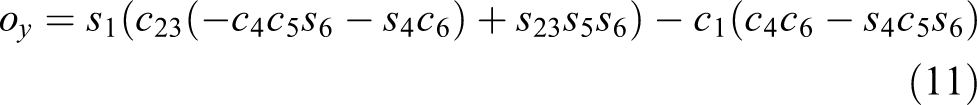
where the entries of T are given by

n_{x} = c_{1} (c_{23} (c_{4} c_{5} c_{6} - s_{4} s_{5}) - s_{23} s_{5} c_{5}) + s_{1} (s_{4} c_{5} c_{6} + c_{4} s_{6})

n_{y} = s_{1} (c_{23} (c_{4} c_{5} c_{6} - s_{4} s_{6}) - s_{23} s_{5} c_{6}) + c_{1} (s_{4} c_{5} c_{6} + c_{4} s_{6})

n_{z} = - s_{23} (c_{4} c_{5} c_{6} - s_{4} s_{6}) - c_{23} s_{5} c_{6}

o_{x} = c_{1} (c_{23} (- c_{4} c_{5} s_{6} - s_{4} c_{6}) + s_{23} s_{5} s_{6}) + s_{1} (c_{4} c_{6} - s_{4} c_{5} s_{6})

o_{y} = s_{1} (c_{23} (- c_{4} c_{5} s_{6} - s_{4} c_{6}) + s_{23} s_{5} s_{6}) - c_{1} (c_{4} c_{6} - s_{4} c_{5} s_{6})

o_{z} = - s_{23} (- c_{4} c_{5} s_{6} - s_{4} c_{6}) + c_{23} s_{5} c_{6}

a_{x} = - c_{1} (c_{23} c_{4} s_{5} + s_{23} c_{5}) - s_{1} s_{4} s_{5}

a_{y} = - s_{1} (c_{23} c_{4} s_{5} + s_{23} c_{5}) + c_{1} s_{4} s_{5}

a_{z} = s_{23} c_{4} s_{5} - c_{23} c_{5}

x = c_{1} (a_{2} c_{2} + a_{3} c_{23} - d_{4} s_{23}) - d_{3} s_{1}

y = s_{1} (a_{2} c_{2} + a_{3} c_{23} - d_{4} s_{23}) + d_{3} c_{1}

z = - a_{3} s_{23} - a_{2} s_{2} - d_{4} c_{23} .

It is used $s_{23}$ for $sin (θ_{2} + θ_{3})$ and $c_{23}$ for $cos (θ_{2} + θ_{3})$ .

According to Craig,²³ for the solution of IK of a robotic manipulator with six degrees of freedom, there are 12 equations and 6 unknowns. However, among the nine equations that arise from the portion of the rotational matrix of $T,$ only three are independent. These, added to the equations of the portion of the position vector of T, result in six equations with six unknowns. Such equations are nonlinear, transcendental, which can be quite difficult to solve.

The systematic approach to solve kinematic equations, proposed by Paul,⁹ rewrites FK equations in several different ways. Thus, both sides of the FK matrix equation are left and right multiplied by inverse transformation matrices. In doing so, one gets equivalent equations having the same solutions. Each matrix equation provides 12 nonlinear equations from the three main matrix lines. The fourth line of the matrix is always trivial. The main problem is to find, in this universe, suitable equations that can be solved analytically.

The solution of IK of this robotic manipulator, as determined by Craig,²³ is given by equations to

θ_{1} = Atan 2 (y, x) - Atan 2 (d_{3}, \pm \sqrt{x^{2} + y^{2} - d_{3}^{2}})

θ_{3} = Atan 2 (a_{3}, d_{4}) - Atan 2 (\begin{matrix} (\frac{x^{2} + y^{2} + z^{2} - a_{2} ​^{2} - a_{3} ​^{2} - d_{3} ​^{2} - d_{4} ​^{2}}{2 a_{2}}), \\ \pm \sqrt{a_{3} ​^{2} + d_{4} ​^{2} - {(\frac{x^{2} + y^{2} + z^{2} - a_{2} ​^{2} - a_{3} ​^{2} - d_{3} ​^{2} - d_{4} ​^{2}}{2 a_{2}})}^{2}} \end{matrix})

θ_{2} = Atan 2 ((- a_{3} - a_{2} c_{3}) z - (c_{1} x + s_{1} y) (d_{4} - a_{2} s_{3}), (a_{2} s_{3} - d_{4}) z - (a_{3} + a_{2} c_{3}) (c_{1} x + s_{1} y)) - θ_{3}

θ_{4} = Atan 2 ((- a_{x} s_{1} + a_{y} c_{1}), (- a_{x} c_{1} c_{23} - a_{y} s_{1} c_{23} + a_{z} s_{23}))

θ_{4}' = θ_{4} + π

θ_{5} = \pm Atan 2 (- (a_{x} (c_{1} c_{23} c_{4} + s_{1} s_{4}) + a_{y} (s_{1} c_{23} c_{4} - c_{1} s_{4}) - a_{z} (s_{23} c_{4})), (a_{x} (- c_{1} s_{23}) + a_{y} (- s_{1} s_{23}) + a_{z} (- c_{23})))

θ_{6} = Atan 2 (\begin{matrix} (- n_{x} (c_{1} c_{23} s_{4} - s_{1} c_{4}) - n_{y} (s_{1} c_{23} s_{4} + c_{1} c_{4}) + n_{z} (s_{23} s_{4})), \\ (n_{x} ((c_{1} c_{23} c_{4} + s_{1} s_{4}) c_{5} - c_{1} s_{23} s_{5}) + n_{y} (((s_{1} c_{23} c_{4} - c_{1} s_{4}) c_{5}) - s_{1} s_{23} s_{5}) - n_{z} (c_{4} s_{23} c_{5} + s_{1} c_{23} c_{4} s_{5})) \end{matrix})

θ_{6}' = θ_{6} + π

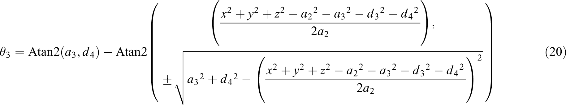
All the equations of the FK and IK of the PUMA 560 manipulator were deduced in detail by Craig²³ and Ghosal.²¹

The tree structure in Figure 4 represents the order of computations to determine all eight joint configurations of the PUMA 560.

Figure 4.

Echelon form of the eight inverse kinematics configurations of PUMA 560.

To measure the computational cost to determine all joint configurations to position and orient the end-effector arbitrarily in the space, the following joint values: $θ = [- \frac{5 π}{6}, \frac{π}{2}, 0, π, \frac{π}{2}, \frac{π}{6}]$ rad and the nonzero parameters: $a_{2} = 432$ , $a_{3} = 20$ , $d_{3} = 125$ , and $d_{4} = 430$ were replaced in equation (5), thus obtaining equation (27)

T = [\begin{matrix} 1 & 0 & 0 & \frac{125}{2} + 215 \sqrt{3} \\ 0 & - 1 & 0 & 215 - \frac{125 \sqrt{3}}{2} \\ 0 & 0 & - 1 & - 452 \\ 0 & 0 & 0 & 1 \end{matrix}]

From this point, equations (7) to (18) have been rewritten by substituting n_x, n_y, n_z, o_x, o_y, o_z, a_x, a_y, a_z, x, y, and z by the respective values of the obtained numerical matrix.

The Solve command in MAPLE is used to find all the values of $θ = [θ_{1}, θ_{2}, θ_{3}, θ_{4}, θ_{5}, θ_{6}]$ , which allow the robot to assume the configuration given by equation (27).

Performing 34,514 floating-point operations (2409 additions, 4261 multiplications, 175 divisions, and 3393 functions), eight different joint configurations are obtained, as given in Table 2.

Table 2.

Joint configurations of the Puma 560, determined through Paul’s method.

$θ_{1} (rad)$	$θ_{2} (rad)$	$θ_{3} (rad)$	$θ_{4} (rad)$	$θ_{5} (rad)$	$θ_{6} (rad)$
−2.617993878	3.091716375	−3.048636391	3.141592654	0.04307998349	0.523598777
−2.617993878	3.091716375	−3.048636391	0	−0.04307998349	−2.617993878
−0.04220293154	1.570796328	−3.048636391	0	1.477840064	−0.04220293154
−0.04220293154	1.570796328	−3.048636391	3.141592654	−1.477840064	3.099389722
−2.617993878	1.570796328	0.00000000008	0	−1.570796328	−2.617993878
−2.617993878	1.570796328	0.00000000008	3.141592654	1.570796328	0.523598777
−0.04220293154	0.04987627939	0.00000000008	0	−0.04987627939	−0.04220293154
−0.04220293154	0.04987627939	0.00000000008	3.141592654	0.04987627939	3.099389722

This article will prove that using Gröbner bases theory, the computational cost to determine the solution of the IK of serial manipulators is considerably reduced.

Inverse kinematics using Gröbner bases theory

The IK problem consists of finding all combinations of joint configurations that will position the end-effector of a robot at a given point in space.²³ To solve this problem, one must determine polynomial equations that model the movement of the robotic arm in each joint configuration. With all these elements, one must seek a set of solutions from the possible movements of each joint.

The joint values are set to $θ = [- \frac{5 π}{6}, \frac{π}{2}, 0, π, \frac{π}{2}, \frac{π}{6}]$ rad, and the parameters are set to $a_{2} = 432$ , $a_{3} = 20$ , $d_{3} = 125$ , and $d_{4} = 430$ in equation (5), exactly as in the third section, to determine all joint configurations to position and orient the end-effector of PUMA 560 robotic manipulator in space.

From this point, equations (7) to (18) are rewritten by substituting n_x, n_y, n_z, o_x, o_y, o_z, a_x, a_y, a_z, x, y, and z by the respective values of the matrix (27). These 12 polynomials, added to the six polynomials obtained from the fundamental trigonometric relation for each joint angle, are used to generate a Gröbner basis.

The selected lexicographic order for this robot is the one shown in equation (28). This order represents the same sequence in which the variables were solved while applying Paul’s method presented in the third section

c_{6} ≻ s_{6} ≻ c_{5} ≻ s_{5} ≻ c_{4} ≻ s_{4} ≻ c_{2} ≻ s_{2} ≻ c_{3} ≻ s_{3} ≻ c_{1} ≻ s_{1} .

The same values assigned in the third section are used, intending to compare the computational efficiency to solve the IK problem using Paul’s method from the Denavit–Hartenberg matrix and Gröbner bases theory of the same 6R manipulator.

Performing 466 floating-point operations (46 additions, 100 multiplications, and 40 functions), the following Gröbner basis consisting of 12 polynomials is obtained using Faugère’s F4 algorithm²⁰

g_{1} = 8600 \sqrt{3} s_{1} + 32084 s_{1} ​^{2} + 4300 \sqrt{3} + 2500 s_{1} - 6771

g_{2} = - 8021 \sqrt{3} s_{1} - 1250 \sqrt{3} + 5521 c_{1} - 8600 s_{1} - 4300

g_{3} = 1853 s_{3} ​^{2} + 172 s_{3}

g_{4} = 2 c_{3} - 43 s_{3} - 2

\begin{matrix} g_{5} = 18578641250 s_{1} s_{3} \sqrt{3} + 862257500 \sqrt{3} s_{1} \\ + 9289320625 \sqrt{3} s_{3} + 63910525900 s_{1} s_{3} \\ + 431128750 \sqrt{3} + 2966165800 s_{1} \\ + 2148795284 s_{2} + 9959875000 s_{3} - 665712384 \end{matrix}

g_{6} = - 226593250 \sqrt{3} s_{1} - 113296625 \sqrt{3} + 537198821 c_{2} - 779480780 s_{1} - 5780183345 s_{3} - 389740390

g_{7} = s_{4}

g_{8} = c_{4} ​^{2} - 1

\begin{matrix} g_{9} = 433134000 c_{4} s_{3} s_{1} \sqrt{3} - 431128750 s_{1} c_{4} \sqrt{3} \\ + 216567000 c_{4} s_{3} \sqrt{3} + 1489980960 c_{4} s_{3} s_{1} \\ - 215564375 \sqrt{3} c_{4} - 1483082900 s_{1} c_{4} \\ + 11821264848 c_{4} s_{3} + 332856192 c_{4} + 1074397642 s_{5} \end{matrix}

\begin{matrix} g_{10} = - 4656190500 s_{1} s_{3} \sqrt{3} - 226593250 \sqrt{3} s_{1} \\ - 2328095250 \sqrt{3} s_{3} - 16017295320 s_{1} s_{3} \\ - 113296625 \sqrt{3} + 537198821 c_{5} \\ - 779480780 s_{1} - 2226636864 s_{3} - 389740390 \end{matrix}

g_{11} = - c_{4} s_{1} + s_{6}

g_{12} = - 8021 s_{1} c_{4} \sqrt{3} - 1250 \sqrt{3} c_{4} - 8600 s_{1} c_{4} - 4300 c_{4} + 5521 c_{6}

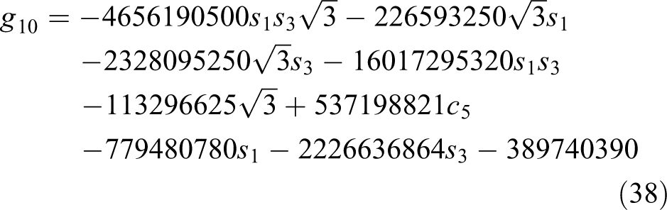
It is worth noting that this reduced number of polynomials, compared to the 72 polynomials found by Wang et al.,¹⁴ will positively reflect on the computational efficiency for the IK solution of a 6R serial manipulator.

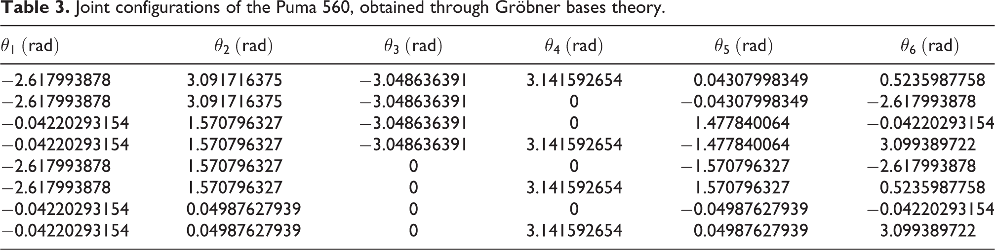
To determine all the values of $θ = [θ_{1}, θ_{2}, θ_{3}, θ_{4}, θ_{5}, θ_{6}]$ , the Solve command is used in MAPLE. Eight different joint configurations are obtained, performing 954 floating-point operations (46 additions, 100 multiplications, and 101 functions), as can be seen in Table 3. These are approximately the same configurations obtained in Table 2.

Table 3.

Joint configurations of the Puma 560, obtained through Gröbner bases theory.

$θ_{1} (rad)$	$θ_{2} (rad)$	$θ_{3} (rad)$	$θ_{4} (rad)$	$θ_{5} (rad)$	$θ_{6} (rad)$
−2.617993878	3.091716375	−3.048636391	3.141592654	0.04307998349	0.5235987758
−2.617993878	3.091716375	−3.048636391	0	−0.04307998349	−2.617993878
−0.04220293154	1.570796327	−3.048636391	0	1.477840064	−0.04220293154
−0.04220293154	1.570796327	−3.048636391	3.141592654	−1.477840064	3.099389722
−2.617993878	1.570796327	0	0	−1.570796327	−2.617993878
−2.617993878	1.570796327	0	3.141592654	1.570796327	0.5235987758
−0.04220293154	0.04987627939	0	0	−0.04987627939	−0.04220293154
−0.04220293154	0.04987627939	0	3.141592654	0.04987627939	3.099389722

It is worth noting that all the equations presented in the third section, using Paul’s method to solve the IK of the PUMA 560 manipulator, were calculated using the computer algebra system MAPLE performing 34,514 floating-point operations to determine the eight different configurations, as given in Table 2.

Adding the 466 floating-point operations to obtain the Gröbner basis to the number of floating-point operations to obtain the eight different joint configurations through the generated Gröbner basis (954 flop), 1420 floating-point operations are obtained. There was a reduction from 34,514 to 1420 in the number of floating-point operations performed to solve the IK problem for this set of configurations.

Performance analysis

To confirm the computational efficiency for the solution of the IK of anthropomorphic robotic manipulators using Gröbner bases theory, 19 new joint configurations will be analyzed. The following joint values are used: $[0, 0, 0, 0, 0, 0],$ $[\frac{π}{6}, \frac{π}{3}, - \frac{π}{6}, \frac{2 π}{3}, \frac{π}{3}, - \frac{π}{3}]$ , $[0, - \frac{π}{6}, 0, \frac{π}{3}, - \frac{2 π}{3}, 0]$ , $[\frac{π}{6}, - \frac{π}{6}, \frac{π}{6}, - \frac{π}{6}, \frac{π}{6}, - \frac{π}{6}]$ , $[\frac{π}{6}, - \frac{π}{6}, 0, 0, 0, - \frac{π}{6}]$ , $[0, 0, \frac{π}{2}, - \frac{π}{2}, 0, \frac{π}{2}]$ , $[- \frac{π}{2}, \frac{π}{2}, 0, - π, - \frac{π}{2}, \frac{π}{6}]$ , $[- \frac{π}{3}, \frac{π}{6}, \frac{π}{3}, \frac{2 π}{3}, \frac{π}{2}, - \frac{π}{2}]$ , $[0, \frac{π}{3}, - \frac{π}{6}, \frac{2 π}{3}, - \frac{π}{2}, \frac{π}{2}]$ , $[0, \frac{π}{3}, - \frac{π}{2}, \frac{π}{2}, 0, \frac{π}{2}]$ , $[\frac{π}{2}, 0, 0, - \frac{π}{2}, 0, \frac{π}{2}]$ , $[\frac{π}{6}, - \frac{π}{6}, \frac{π}{6}, - \frac{π}{6}, \frac{π}{6}, - \frac{π}{6}]$ , $[\frac{π}{3}, - \frac{π}{6}, \frac{π}{2}, - \frac{π}{2}, \frac{2 π}{3}, - \frac{π}{2}]$ , $[\frac{π}{6}, - \frac{π}{3}, \frac{π}{2}, \frac{π}{2}, - \frac{π}{3}, 0]$ , $[\frac{π}{6}, - \frac{π}{3}, 0, 0, - \frac{π}{3}, 0]$ , $[\frac{π}{2}, \frac{5 π}{6}, 0, \frac{π}{3}, - \frac{π}{3}, \frac{π}{2}]$ , $[\frac{π}{3}, \frac{5 π}{6}, - \frac{π}{6}, \frac{π}{3}, - \frac{π}{3}, - \frac{π}{2}]$ , $[0, \frac{5 π}{6}, 0, \frac{π}{3}, - \frac{π}{3}, - \frac{π}{2}]$ , and $[\frac{π}{6}, \frac{π}{2}, - \frac{π}{6}, \frac{π}{3}, - \frac{π}{2}, \frac{π}{6}]$ .

Unlike the results presented by Guzmán-Giménez et al.,¹² all joint configurations provide the same amount of solutions determined by Paul’s method. The two methods were simulated in MAPLE, testing their ability to solve the IK problem, and all the 100 solutions obtained for both methods were compared, testing their efficiency in solving.

Comparisons of the number of mathematical operations performed using the two methods are shown in Figure 5. The x-axis presents a partition of 20 sets used to determine 100 different configurations for the PUMA 560 using Paul’s method and Gröbner bases theory, while the y-axis shows the total number of operations performed on a logarithmic scale.

Figure 5.

(a–d) Amount of operations performed using the two methods.

The performance comparisons of the two methods are shown in Figure 6. The x-axis presents a partition of 20 sets used to determine 100 different configurations for the PUMA 560 using both methods, while the y-axis shows the total number of floating-point operations on a logarithmic scale.

Figure 6.

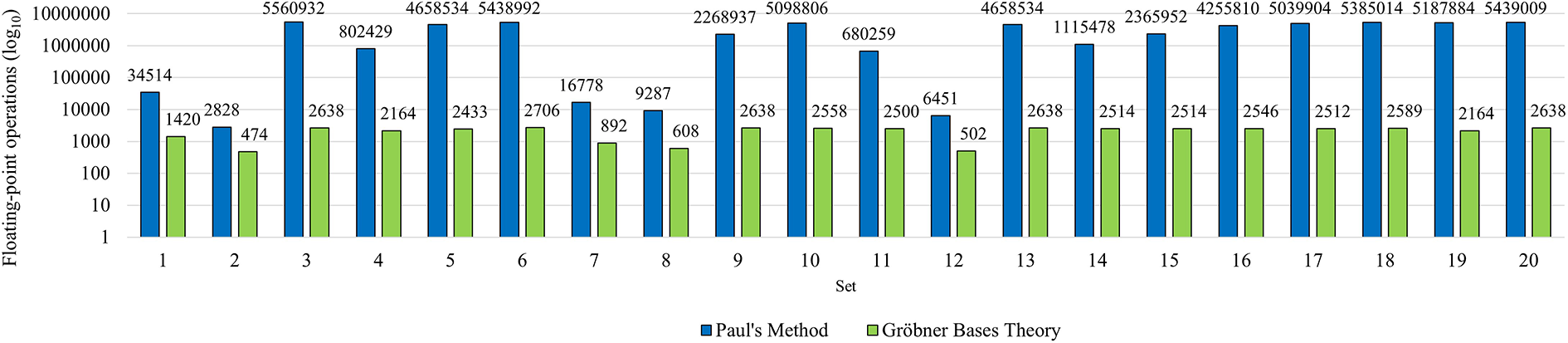
Performance comparisons of the two methods.

It was possible to observe in Figure 5 that there was a significant reduction in the number of mathematical operations to obtain all solutions using Gröbner bases theory. As expected, the number of floating-point operations is reduced, as shown in Figure 6.

The histogram of the RMS errors in the calculations of all six joint angles of the PUMA 560 manipulator in all analyzed configurations is shown in Figure 7. The x-axis presents a partition of 100 sets of the obtained root mean square (RMS) errors in ascending order, while the y-axis shows the frequency of occurrence of each of these error sets. The RMS error is approximately $8.14 \times 10^{- 10}$ rad.

Figure 7.

Histogram of the RMS errors in the computations of all six joint angles of the PUMA 560. RMS: root mean square.

It can be verified in the histogram presented that most of the obtained RMS errors occur within the first sets, the ones that represent less error. It can also be seen that the higher sets still represent very insignificant errors. Figure 8 shows the simulation results of joint variable errors in all 100 configurations analyzed.

Figure 8.

Simulation results of joint variables errors. (a) θ₁, (b) θ₂, (c) θ₃, (d) θ₄, (e) θ₅, and (f) θ₆.

The comparative analysis of IK solutions is shown in Figure 9. The red dots represent the angles obtained through Paul’s method for each joint, while the continuous blue lines represent the angles obtained through Gröbner bases theory. The data show that the outputs follow those obtained by Paul’s method with high accuracy and a negligible error.

Figure 9.

Comparative analysis of inverse kinematics solutions ( $θ_{1}$ to $θ_{6}$ ): (a) θ₁, (b) θ₂, (c) θ₃, (d) θ₄, (e) θ₅, and (f) θ₆.

The histograms of the RMS errors in the calculations of all positions and rotation angles of the end-effector of the PUMA 560 are shown in Figure 10. The x-axis presents a partition of 100 sets of the obtained RMS errors, while the y-axis shows the frequency of occurrence of each of these error sets. The RMS error obtained is $4.34 \times 10^{- 7}$ mm for the position and $1.27 \times 10^{- 9}$ rad for the orientation of the robot’s end-effector.

Figure 10.

Histograms of the RMS errors in the computations of all positions and rotation angles of the end-effector. RMS: root mean square.

All the histograms presented (Figures 7 and 10) show that most of the obtained RMS errors occur within the first sets, the ones that represent less error. It can also be seen that the higher sets still represent a completely insignificant error.

Figure 11 shows the simulation results of positioning and orientation errors in all 100 configurations analyzed.

Figure 11.

(a–f) Results of simulation of positioning and orientation errors.

The comparative analysis of FK solutions is shown in Figure 12. The green dots represent the x, y, and z coordinates of the points obtained from the angles determined through Paul’s method, while the solid orange lines represent the coordinates of the points obtained from the angles determined through Gröbner bases theory. The blue dots represent the rotation angles obtained from the angles determined through Paul’s method, while the solid red lines represent the rotation angles obtained from the angles determined through Gröbner bases theory. The data show that the results continue to maintain high accuracy and negligible error.

Figure 12.

(a–f) Comparative analysis of forward kinematics solutions.

El-Sherbiny et al.¹⁶ presented a comparative study between three different soft-computing-based methods (artificial neural network, adaptive neuro-fuzzy inference system, and genetic algorithms) applied to the problem of IK. The analysis results demonstrate that the methods are not accurate and computationally efficient at the same time. Using the artificial neural network method with a minimized error function and the adaptive neuro-fuzzy inference system method with the same function, the calculation time is quite similar. The difference is in the accuracy of the end-effector position and the angle of rotation. When the genetic algorithm method is used, the position error is very low, which is less than $10^{- 3}$ mm, while the calculation time is high compared to the other methods.

It is worth mentioning that in this work, the RMS error obtained is $4.34 \times 10^{- 7}$ mm for the position of the end-effector and $1.27 \times 10^{- 9}$ rad for the orientation of the end-effector. As shown in Figure 12, the solutions obtained through Gröbner bases theory produce negligible positioning and orientation errors in all configurations.

Open problem: Analysis of singularities

Stifter¹⁹ presented an algorithm to solve the IK of a 2R robot using Gröbner bases theory. The author presented a brief list of subjects that were not yet fully resolved but that could play an essential role in applying Gröbner bases theory for solving the problem of IK. The question about the possibility of determining singular configurations using a Gröbner basis is highlighted in this list.

Kendricks¹¹ used a Gröbner basis to determine the occurrence of a singularity of the workspace boundary, configuration when the manipulator is fully extended to the outer boundary or fully retracted to the inner boundary of its workspace. Her analysis focused on the robot Fanuc A-510, a SCARA type robot with three degrees of freedom, analyzing the discriminant of quadratic polynomials on the Gröbner basis generated to solve the IK of this serial robot. In this case, the author determined intervals of angles that produce a single real solution, whose discriminants in the quadratic equations are equal to zero.

The anthropomorphic robot Unimation PUMA 560, used as a case study in this work, has the last three axes intersecting at a point. As a consequence, the position of the end-effector is only a function of $θ_{1}$ , $θ_{2}$ , and $θ_{3}$ . In this way, the following three nonlinear equations in three unknowns are used

x = c_{1} (a_{2} c_{2} + a_{3} c_{23} - d_{4} s_{23}) - d_{3} s_{1}

y = s_{1} (a_{2} c_{2} + a_{3} c_{23} - d_{4} s_{23}) + d_{3} c_{1}

z = - a_{3} s_{23} - a_{2} s_{2} - d_{4} c_{23}

To check whether it is possible to determine from a Gröbner base whether there is a singularity, equations (41) to (43) are rewritten by substituting x, y, and z by the respective values of the matrix (27). These three polynomials, added to the three polynomials obtained from the fundamental trigonometric relation for each joint variable, are used to generate a Gröbner basis.

The selected lexicographic order for this robot is the one shown in equation (44). This order represents the same sequence in which the first three joint variables were solved while applying Paul’s method presented in the third section

c_{2} ≻ s_{2} ≻ c_{3} ≻ s_{3} ≻ c_{1} ≻ s_{1}

The following Gröbner basis consisting of six polynomials is obtained using Faugère’s F4 algorithm²⁰

g_{1} = (x^{2} + y^{2}) s_{1} ​^{2} + 250 x s_{1} - y^{2} + 15625

g_{2} = c_{1} y - s_{1} x - 125

\begin{matrix} g_{3} = 138325708800 s_{3} ​^{2} + (743040 x^{2} + 743040 y^{2} \\ + 743040 z^{2} - 287964408960) s_{3} + x^{4} + 2 x^{2} y^{2} \\ + 2 z^{2} x^{2} + y^{4} + 2 y^{2} z^{2} + z^{4} - 775098 x^{2} \\ - 775098 y^{2} - 775098 z^{2} + 149895629001 \end{matrix}

g_{4} = - x^{2} - y^{2} - z^{2} + 17280 c_{3} - 371520 s_{3} + 387549

\begin{matrix} g_{5} = (16009920 x^{2} + 16009920 y^{2}) s_{1} s_{3} \\ + (43 x^{4} + 86 x^{2} y^{2} + 43 x^{2} z^{2} + 43 y^{4} + 43 y^{2} z^{2} \\ - 16664607 x^{2} - 16664607 y^{2}) s_{1} \\ + (1728 x^{2} y + 1728 y^{3} + 1728 y z^{2} - 27000000 y) s_{2} \\ + 2001240000 x s_{3} + 2 x^{2} y z + 2 y^{3} z + 2 y z^{3} + 5375 x^{3} \\ + 5375 x y^{2} + 5375 z^{2} x - 28602 y z - 2083075875 x \end{matrix}

\begin{matrix} g_{6} = (1728 x^{2} y + 1728 y^{3} + 1728 y z^{2} - 27000000 y) c_{2} \\ + (- 2 x^{4} - 4 x^{2} y^{2} - 2 x^{2} z^{2} - 2 y^{4} - 2 y^{2} z^{2} + 28602 x^{2} \\ + 28602 y^{2}) s_{1} + 16009920 s_{3} y z + 43 x^{2} y z + 43 y^{3} z \\ + 43 y z^{3} - 250 x^{3} - 250 x y^{2} - 250 z^{2} x - 16664607 y z \\ + 3575250 x \end{matrix}

Note that the first element in the basis is a quadratic polynomial in terms of s₁. By examining the discriminant of this equation, it can be observed that there will be no real solutions for s₁, when

4 y^{2} (x^{2} + y^{2} - 15625) < 0

Moreover, by analyzing the discriminant of the third element in the basis, there will be no real solutions to s₃ when

- x^{4} - 2 x^{2} y^{2} - 2 x^{2} z^{2} + 775098 x^{2} - y^{4} - 2 y^{2} z^{2} + 775098 y^{2} - z^{4} + 775098 z^{2} - 11868518601 < 0

To obtain a quadratic polynomial in terms of s₂, a new lexicographic order for this robot is used: $c_{3} ≻ s_{3} ≻ c_{2} ≻ s_{2} ≻ c_{1} ≻ s_{1}$ . The following Gröbner basis consisting of six polynomials is obtained using Faugère’s F4 algorithm²⁰

g_{1} = (x^{2} + y^{2}) s_{1} ​^{2} + 250 x s_{1} - y^{2} + 15625

g_{2} = c_{1} y - s_{1} x - 125

\begin{matrix} g_{3} = (746496 x^{2} + 746496 y^{2} + 746496 z^{2} - 11664000000) s_{2} ​^{2} \\ + (1728 x^{2} z + 1728 y^{2} z + 1728 z^{3} - 24712128 z) s_{2} \\ + x^{4} + 2 x^{2} y^{2} + 2 z^{2} x^{2} + y^{4} + 2 y^{2} z^{2} + z^{4} - 775098 x^{2} \\ - 775098 y^{2} - 28602 z^{2} + 11868518601 \end{matrix}

\begin{matrix} g_{4} = (864 x^{2} y + 864 y^{3} - 13500000 y) c_{2} \\ + (- 864 x^{2} z - 864 y^{2} z) s_{1} s_{2} + (- x^{4} - 2 x^{2} y^{2} \\ - x^{2} z^{2} - y^{4} - y^{2} z^{2} + 14301 x^{2} + 14301 y^{2}) s_{1} \\ - 108000 x z s_{2} - 125 x^{3} - 125 x y^{2} - 125 z^{2} x + 1787625 x \end{matrix}

\begin{matrix} g_{5} = (1728 x^{4} + 3456 x^{2} y^{2} + 1728 x^{2} z^{2} + 1728 y^{4} \\ + 1728 y^{2} z^{2} - 27000000 x^{2} - 27000000 y^{2}) s_{1} s_{2} \\ + (2 x^{4} z + 4 x^{2} y^{2} z + 2 x^{2} z^{3} + 2 y^{4} z + 2 y^{2} z^{3} - 28602 x^{2} z \\ - 28602 y^{2} z) s_{1} + (216000 x^{3} + 216000 x y^{2} + 216000 x z^{2} \\ - 3375000000 x) s_{2} + (16009920 x^{2} y + 16009920 y^{3} \\ - 250155000000 y) s_{3} + 43 x^{4} y + 86 x^{2} y^{3} + 43 x^{2} y z^{2} \\ + 43 y^{5} + 43 y^{3} z^{2} + 250 x^{3} z + 250 x y^{2} z + 250 x z^{3} \\ - 17336482 x^{2} y - 17336482 y^{3} - 671875 y z^{2} \\ - 3575250 x z + 260384484375 y \end{matrix}

\begin{matrix} g_{6} = (16009920 x^{2} y + 16009920 y^{3} - 250155000000 y) c_{3} \\ + (37152 x^{4} + 74304 x^{2} y^{2} + 37152 x^{2} z^{2} + 37152 y^{4} \\ + 37152 y^{2} z^{2} - 580500000 x^{2} - 580500000 y^{2}) s_{1} s_{2} \\ + (43 x^{4} z + 86 x^{2} y^{2} z + 43 x^{2} z^{3} + 43 y^{4} z + 43 y^{2} z^{3} \\ - 614943 x^{2} z - 614943 y^{2} z) s_{1} \\ + (4644000 x^{3} + 4644000 x y^{2} + 4644000 x z^{2} \\ - 72562500000 x) s_{2} - 2 x^{4} y - 4 x^{2} y^{3} - 2 x^{2} y z^{2} - 2 y^{5} \\ - 2 y^{3} z^{2} + 5375 x^{3} z + 5375 x y^{2} z + 5375 x z^{3} + 806348 x^{2} y \\ + 806348 y^{3} + 31250 y z^{2} - 76867875 x z - 12110906250 y \end{matrix}

Note that the third element in the basis is a quadratic polynomial in terms of s₂. By examining the discriminant of this equation, it can be observed that there will be no real solutions for s₂, when

\begin{matrix} - (2985984 (x^{2} + y^{2} - 15625)) (x^{4} + (2 y^{2} + 2 z^{2} - 775098) x^{2} \\ + y^{4} + (2 z^{2} - 775098) y^{2} + z^{4} - 775098 z^{2} + 11868518601) < 0 \end{matrix}

When it is possible to determine an analytical solution for the IK of a manipulator robot using Gröbner bases theory, given a point $(x; y; z)$ , it can determine the maximum number of geometric configurations to position the end-effector of the robot, and, more importantly, it is possible to discover all the real solutions that produce these settings.

However, it is essential to highlight that when all six joint variables are considered in the model, the 6R manipulator presents more than four solutions; however, the Gröbner bases method does not produce analytical solutions, thus requiring numerical methods to find the final solution. In many industry fields, the determination of all rotation angles of the end-effector is indispensable; thus, it justifies the importance of determining all joint angles of a robotic manipulator.

Furthermore, although it is possible to determine angular intervals that produce points that are external to the manipulator’s workspace, singularities such as boundary singularity or inner singularity remain to be further studied.

Conclusions

When using the Gröbner bases method for the solution of IK of anthropomorphic robots, one notes in the tests performed during this research that it is computationally more efficient than Paul’s method since the equations produced for determination of six variables are mathematically simpler to be solved. Since through retroactive substitutions, all joint solutions can be determined to precisely position and orient the robotic manipulator end-effector in space.

According to the performance data obtained (number of floating-point operations) in all the configurations analyzed, it can be stated that the method proposed in this work for the solution of IK of anthropomorphic robots is more efficient computationally than Paul’s method.

In future work, it is intended to demonstrate that this method can also be computationally efficient compared to the other methods for solving the IK problem of redundant manipulators.

Footnotes

Code availability

The MAPLE source code data used to support the findings of this study are available from the corresponding author upon request.

Data availability

The data that support the findings of this study are available from the corresponding author upon request.

Declaration of conflicting interests

The author(s) declared no potential conflicts of interest with respect to the research, authorship, and/or publication of this article.

Funding

The author(s) disclosed receipt of the following financial support for the research, authorship, and/or publication of this article: This study was supported in part by the Coordenação de Aperfeiçoamento de Pessoal de Nível Superior—Brasil (CAPES) (Finance Code 001).

ORCID iD

Sérgio Ricardo Xavier da Silva

References

Daya

Khawandi

Akoum

. Applying neural network architecture for inverse kinematics problem in robotics. J Softw Eng Appl 2010; III: 230–239.

Paul

Shimano

Mayer

. Kinematic control equations for simple manipulators. IEEE Trans Syst Man Cybern 1981; 11: 449–455.

Lee

CSG

. Robot arm kinematics, dynamics, and control. Computer 1982; 15: 62–80.

Yih

Youm

. Geometrical modeling of lower-pairs based on spherical-Euler geometry. Trend Develop Mech Mach Robot 1988; 15: 435–440.

Huang

Milenkovic

. Kinematics of major robot linkages. In: Proceedings of the 13th International Symposium on Industrial Robots; 1983; Chicago: Robotics International of SME, pp. 16–31.

Manseur

Doty

. A fast algorithm for inverse kinematic analysis of robot manipulators. Int J Robot Res 1988; 7: 52–63.

Denavit

Hartenberg

. Description and displacement analysis of mechanics based on the 2 × 2 dual matrices. Evanston: University of Northwestern, 1955.

Hartenberg

Denavit

. Kinematic synthesis of linkages. Col: McGraw-Hill series in mechanical engineering. New York: McGraw-Hill, 1965.

Paul

. Robot manipulators: mathematics, programming, and control (artificial intelligence). Cambridge: MIT Press, 1981.

10.

Buchberger

Bruno Buchberger’s PhD thesis 1965: an algorithm for finding the basis elements of the residue class ring of a zero dimensional polynomial ideal. J Symbol Comput 2006; 41: 475–511.

11.

Kendricks

. Solving the inverse kinematic robotics problem for the GMF-A510 robot: a comparison study of the denavit-hartenberg matrix and groebner basis theory. PhD Thesis, The Graduate School of Auburn University: Auburn University Libraries, Auburn, USA, 2007.

12.

Guzmán-Giménez

Fernández

ÁV

Amela

, et al. Synthesis of the inverse kinematic model of non-redundant open-chain robotic systems using Gröbner basis theory. Appl Sci 2020; 10: 2781.

13.

. 6R robot inverse solution algorithm based on quaternion matrix and Gröbner base. Adv Linear Algebra Matrix Theory 2018; VIII: 33–40.

14.

Wang

Hang

Yang

. Inverse kinematics analysis of general 6r serial robot mechanism based on Gröbner base. Front Mech Eng China 2006; 1(I): 115–124.

15.

Duffy

Crane

. Displacement analysis of the general 7-link 7R mechanism. Mech Mach Theory 1980; XV: 153–169.

16.

El-Sherbiny

Elhosseini

Haikal

. A comparative study of soft computing methods to solve inverse kinematics problem. Ain Shams Eng J 2017; 9. DOI: 10.1016/j.asej.2017.08.001.

17.

Cox

Little

O’Shea

. Ideals, varieties, and algorithms: an introduction to computational algebraic geometry and commutative algebra. 4th ed. New York: Springer, 2015.

18.

Sturmfels

. What is…a Gröbner basis? Not Am Math Soc 2005; 52(10): 1199–1200.

19.

Stifter

. Algebraic methods for computing inverse kinematics. J Intell Robot Syst 1994; 11: 79–89.

20.

Faugère

. A new efficient algorithm for computing Gröbner bases (F4). J Pure Appl Algebra 1999; 139: 61–88.

21.

Ghosal

. Robotics: fundamental concepts and analysis, New Delhi: Oxford University Press, 2006.

22.

Chakravarti

Sivakumar

. A GA-integrated adaptive model reference controller in robot tracking applications. J Multidiscip Eng Sci Studies 2016; 2: 283–291.

23.

Craig

. Introduction to robotics: mechanics and control. (4th ed). Boston: Addison-Wesley, 2017.