
Abstract
This paper proposes a recursive differential evolution (RDE) algorithm to identify the inertial parameters of an unknown target and simultaneously revise the friction parameters of space manipulator joints. The inertia parameters of a space manipulator, which govern the dynamic behaviours of the entire system to a significant extent, can change for many reasons during the process of on-orbit operations; consequently, it is essential to trace these changes within the control system to ensure the stability and accuracy of the entire system. RDE is inspired by a recursive least squares algorithm, using approximate gradient information to guide the mutation operation in the standard DE. A series of contrast simulations are employed to confirm the feasibility of the RDE algorithm. The simulation results show that the identification of the RDE algorithm is more precise than for a GA (genetic algorithm) and LS (least square) algorithm, and has an appropriate convergence rate. The RDE identification method is suitable for linear, nonlinear and combined systems, and can follow system dynamics exactly.
1. Introduction
Space robotics is considered one of the most promising approaches for on-orbit servicing (OOS) missions such as docking, berthing, refuelling, repairing, upgrading, transporting, rescuing, orbital debris removal, etc. Many enabling techniques have been developed in the past two decades and several technology demonstration missions have been completed [1, 2]. A number of on-orbit servicing missions have been successfully accomplished. Engineering Test Satellite VII (ETS-VII), an unmanned spacecraft equipped with a 2m long, six-degree-of-freedom manipulator arm, with the objective of verifying technologies for autonomous rendezvous and docking (AR&D), as well as robotic servicing in space [3], was developed and launched by the National Space Development Agency of Japan (NASDA). ETS-VII has successfully carried out a variety of on-board experiments with its manipulator arm, such as model-based space robot teleoperation from the ground with a time-delay [4] and robotic servicing tasks such as orbital replacement units (ORU) exchange, deployment of a space structure, and capture and berthing of a target satellite [5]. These key technologies are essential for an orbital free-flying robot. The Defence Advanced Research Projects Agency (DARPA), in conjunction with Boeing, successfully launched and accomplished the Orbital Express mission in 2007. As an advanced OOS technology demonstration mission, it demonstrated short-range and long-range autonomous rendezvous, capture and berthing, on-orbit electronics upgrades, on-orbit refuelling, as well as an autonomous fly-around visual inspection using a demonstration client satellite. During the mission, a robotic arm autonomously transferred a supplemental battery and backup computer to a target spacecraft designed to be serviced [6].
During the process of the on-orbit operations, the inertia parameters of the space robot can change for several reasons, e.g., fuel consumption, payload deployment, capturing of a target or docking with a spacecraft. The control system should trace the changes of these parameters to ensure the stability and accuracy of the entire system. For example, the inertia parameters of the combination of manipulator arm and target are not the same as for the single manipulator after capturing an unknown target. Some operations of the manipulator cannot be completed optimally if the inertia parameters of a new compound system are not well-known. In other cases, advanced control methods that considered the arm/base coupling, such as “reactionless manipulation” [7], resolved motion control based on a “generalized Jacobian matrix” [8] and “coordinated control” [9], etc., need precise knowledge of the inertia parameters of each body [10]. As such, identification of the target and the space manipulator's inertia parameters may become essential.
Generally, knowledge about the 10 inertia parameters such as mass, centre of mass location and the inertia tensor (moments and products of inertia) of mechanical systems is of great interest whenever dynamic behaviour is significantly governed by these parameters [11]. Such parameters are often contained in equations describing the system. There are several methods for identifying the inertia parameters of a robot, most of which are based on Newton-Euler dynamic equations [12–21]. Generally, two assumptions are proposed to correct and identify inertia properties from equations.
The first assumption is that the linear moment and angular moment of the entire system are conserved [12–16]. A procedure has been developed for calculating the mass properties of a manipulator, which is mounted on a six degree-of-freedom force sensor, by measuring the reaction forces and moments at the base. The mass properties identified by this procedure are not sufficiently complete for computed torque and other dynamic control techniques, but do provide compensation for the gravitational load on the links of the manipulator [12]. To avoid the rank deficiency of the identification matrix, a group of the inertia parameters that have a dominant effect on the angular motion dynamics were selected and properly identified [13]. This method enables the inertia parameter identification using standard flight telemetry data of an existing space robot through the simple observation of a typical manipulator operation, and does not require a special measurement apparatus or operation procedure. However, not all of the unknown parameters are identified. By eliminating the linear and angular momenta from the momentum equations, the momentum increment equations are obtained and the unknown inertial parameters of the grasped object are determined [14]. The advantage of this method is that the inertial parameters can be accurately identified in both cases of zero and nonzero momenta and the problem of singular solution can also be avoided. Two approaches—the least square method based on parameter decoupling and the non-linear system optimization based on the PSO, were proposed to identify the inertia parameters of the spacecraft [15]. The approaches do not assume that the spacecraft moves slowly enough and thereby overcome the shortcomings of previous methods that forcibly break the coupling relationship between the parameters. A robotics-based method for on-orbit identification of inertia properties of spacecraft makes use of an on-board robotic arm to change the inertia distribution of the spacecraft system [16]. The velocity of the spacecraft system will change according to inertia redistribution. Since the velocity change is measurable and the inertia redistribution of the robotic arm itself is precisely computable, the inertia parameters of the spacecraft body become the only unknown elements in the momentum equations and hence, can be identified using the momentum equations of the spacecraft system. This method requires accurate kinematics and dynamic parameters of the arm and was insensitive to sensor noise for identifying the mass and mass-centre location, but extremely sensitive to sensor noise for identifying the inertia tensor.
The second assumption is that the space manipulator arm is driven by input torque, which has little influence on the base [17–21]. A method was validated by the ETS-VII satellite experiments using accelerometers [17]. This method consisted of an iteration of three operations: firstly, the planning of optimal manoeuvres with a simulation model and with guessed (or updated) parameters; secondly, execution of the optimal manoeuvres on the real system via data acquisition; finally, identification with a simulation model via updating the parameters. An adaptive control method without using acceleration information in the identification model was proposed [18], which consisted of a PD feedback part and a full dynamics feed- forward compensation part, with the unknown manipulator and payload parameters being estimated online. A neural network was applied to realize online identification, since the sampled real-time data were input to the network in order to obtain the real-time parameter value [19]. The identified parameters were regarded as the weights of the network and the weights approach the actual values of the identified parameters by training the weights. A genetic algorithm, that was able to directly and effectively identify inertial parameters, was applied for inertial parameters identification in the underactuated manipulator system after transformations [20]. An interactive stochastic gradient (ISG) algorithm was proposed to estimate the space manipulators and target inertial parameters in the scenario of multiple space robots manipulating the target [21]. This method utilizes the estimated results between the adjacent nodes to modify locally identified parameters and converges faster and with better robustness and stableness than the distributed least squares method.
In this paper, a method for identifying an unknown target's inertia parameters and correcting the joint friction parameters simultaneously under the second assumption is proposed. In order to estimate the linear and nonlinear dynamic parameters of a space robot in an unknown environment in a timely manner, the new RDE method (recursive differential evolution) is introduced. Compared to traditional algorithms, such as the least square (LS) algorithm, genetic algorithm (GA) and PSO (particle swarm optimization), the RDE algorithm is different in the use of historical information. The current identification results of the traditional algorithms do not has any relationship with the historical results, while the RDE algorithm can utilize the historical results to renew the estimated results. At the same time, the RDE algorithm takes the advantages of DE (Differential Evolution) algorithm such as robustness and fast convergence. In order to use the RDE to solve our problem, at least three improvements/adaptations were made as follows: 1) considering the practical application, we simplified the problem model: the manipulator system was predigested as a two-body system with rigid bodies connected by a rotational joint and the entire system was divided into three sub-body systems, i.e., the unknown body subsystem, the base body subsystem and the two-joint arm body subsystem; 2) in order to make the expression of the manipulator system model equations more concise, we transform the expression form of unknown parameters; 3) consulting the idea of DE/rand-to-best/1/bin mutation strategy and the RLS, the approximate gradient vector of maximum, multiplied by a regulated number, was effected as part of a different vector, which replaced the best vector of DE/rand-to-best/1/bin. This improvement can guide the entire population toward global optimization. Current study achievements primarily focus on linear system identification and nonlinear system off-line identification; however, the RDE algorithm can estimate the dynamic parameters of nonlinear and linear items easily via the different recursive vector updating the system's parameters in a timely manner. The simulation results represent the fine convergent effect of RDE algorithm.
The rest of this paper is organized as follows. In section 2, the dynamic model and its control functions are formulated in consideration of joint friction torque vector. Then, the identified parameters are deduced with the base of dynamic function. In section 3, differential evolution and its improved method are introduced. In section 4, the inspiration for and deduced procedures of RDE are presented. In section 5, RDE is applied to parameter identification for the single-arm space manipulator, before the inertia properties of payload and joint friction coefficient are determined. The simulation and its analysis are also presented in this section. Conclusions and the scope for further research are presented in section 6.
2. Models and Identification Problem
2.1. Models of space manipulator
The space robot system in this paper is considered as a space manipulator with N (or n) degrees of freedom (

Model of space manipulator
In Figure 1, b represents the model of the space manipulator; I (i=1, 2,…n) is the index of the body from the base;
2.2. Dynamic model of space manipulator
When joint friction is considered, the dynamic equations of the space manipulator controlled by the input torque are:

where
When the end effector of the manipulator arm and the target are viewed as a new link of the manipulator, we can obtain

2.3. Model simplification and parameter definition
The configuration of the serial manipulator arm is determined by the joint angles, which can be precisely measured by the joint position sensors. Thus, the exact configuration of the manipulator arm is known at all times. In general, the dynamic parameters of the links and joints, which consist of mass, the centroid position and moments of inertia, will not change with movement of the arm. Therefore, dynamic parameters can be determined in advance and can in practice be considered as constant parameters. The brake device is usually installed on the joints of the manipulator arm for safety. In this way, any of the joints can be individually locked by the brake. For simplicity, we propose the following assumptions: 1) only the first joint and the joint connecting the last two links of the manipulator arm are active and the other joints are locked during the identification process; 2) the exact configuration and the parameters of the links and joints, except the last link, are known.
Figure 2 shows that the entire system is divided into three sub-body systems. The combination of the unknown target and the manipulator arm's final link is known as the unknown body subsystem. The satellite base body is called the base body subsystem and the other of the manipulator arm is called the two-joint arm body subsystem. The base body subsystem and the two-joint arm body subsystem's parameters are known, and these two subsystems are connected by the first joint. Here, the identification parameters are divided by the τl and the τf items.

Simplified model of the space manipulator
Considering the

where

The variables

There is unique corresponding relationship between

Therefore, we can evaluate the parameters
For item τf, the Stribeck model is quoted to analyse the friction torque of joint i: [22]

For joint i,
3. DE Algorithm
3.1. Basic differential evolution
The DE (differential evolution) algorithm is a stochastic, population-based optimization algorithm that was introduced by Storn and Price in 1995 [23]. This algorithm has similar steps to the GA (genetic algorithm), both of which are able to solve practical non-differentiable or non-linear problems, the main difference between them being the mutation strategy. The DE algorithm can adequately employ a group distribution feature to enhance the ability of finding approximate solutions [24]. The procedures of the DE algorithm are as follows:

The initial parameter values

where

The scalar factor

where

3.2. Advanced DE algorithm
The basic DE algorithm mutation strategy is called DE/rand/1/bin [25]. One of the advanced DE algorithms uses the mutation strategy DE/rand-to-best/1/bin:

where combining factor
4. Recursive DE Algorithm
4.1. Inspiration
Let the system model be:

where:

and

where

and

The RLS (recursive least square) algorithm equations are as follows:


where,
The item
Considering the idea of a DE/rand-to-best/1/bin mutation strategy, the approximate gradient vector of the maximum multiplied by a regulated number can be conducted as part of a different vector, which will replace the best vector of DE/rand-to-best/1/bin. This method can guide the entire population
4.2. Deducing process
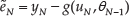
We define the system model as follows:

where

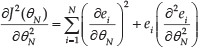
where

Neglect the second-order derivative,

Use Eq.(23) and calculate:

When

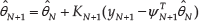
Then, Eq.(23) can be updated by:

Then we update Eq.(24) as:

At moment

As θN is unknown, we use

Take

Clearly, Eq.(34) has a similar form to Eq.(10). This similarity inspired us to use an approximate gradient vector to modify the different vectors. As the item

Experiment results show that including the larger values of
4.3. Comparing DE, ADE & RDE
The primary difference among DE, ADE and RDE is mutation strategy. The RDE algorithm can renew identification parameters when the database is expanded with new data that are suitable to the online problem. The procedures of the three algorithms are shown in Figure 3.

Comparison of DE, ADE and RDE
For the parameter identification problem, as Figure 3 shows, DE and ADE are based only on historical databases, while RDE can employ new data to repeatedly update existing results. RDE uses an off-line identified method to calculate the initializing parameters, as do the DE and ADE, before new data are added to the database.
5. Simulations, Results and Analysis
5.1. Simulation condition
An appropriate driving signal is important for increasing the accuracy of identification results. As the input torque handles the manipulator, the expecting angle position, angle velocity and angle acceleration can be calculated using the physical parameters of the mechanical arm (Table 1), as well as the driving signal τl, in the experiment
Physical parameters of the mechanical arm
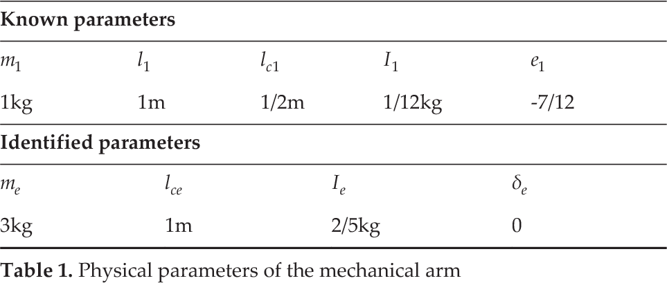
The results of two joints are shown in Figure 4 through Figure 6. Considering the influence of friction torque τf, real torque τ is not the same as the desired values τl. To simplify the simulation process, the undetermined two-joint parameters of τf take the same values that are listed in Table 2.
Undetermined parameters of fc


Joint angle
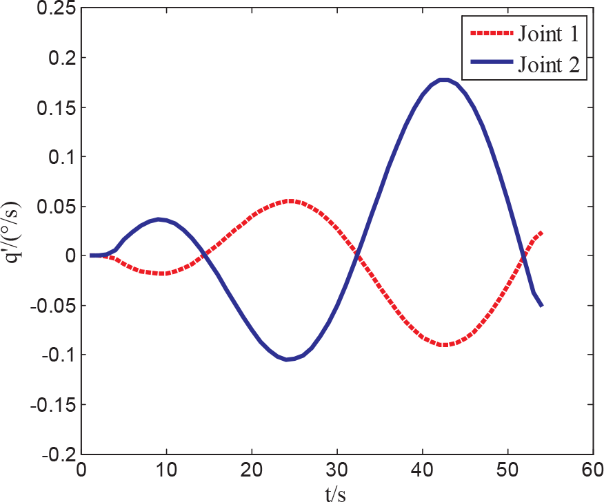
Joint angular velocity

Joint angular acceleration
Some of the simulation experiment's procedures have the opposite sequence to the practical procedures. The values of angle position, angle velocity and the true input torque τ should be measured, sampled and filtered in advance; then, we can discover expected input torque τl and friction torque τf.
Let the parameters
Initial parameter intervals

In order to minimize the estimated difference between real torque values and the calculated torque, we set the objective function as:

5.2. Results and analysis
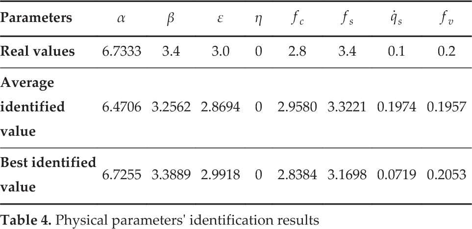
The simulation results are presented in Table 4 and the estimated error variable, alongside recursive times, are shown in Figure 7.
Physical parameters' identification results

Object function value varies according to recursive times
Clearly, the estimated error is large, because the identified parameters are based simply on historical data and the estimated effect is not sufficient. Recent online data, collected from manipulator sensors and added to the database and the RDE gives rise to a progressive and optimizing algorithm; the value of the object function, i.e., the value of the estimated error, decreases against the recursive time, as shown in Figure 7.
The comparison between real input torque and the torque calculated by the identified parameters are shown in Figure 8 and Figure 9. From these representations, we can conclude that the former torque values of the two joints had a small error compared to the real torque values; this occurred due to the estimated error of parameters. Alongside further estimation of the parameters, the estimated error values decrease and the estimated torque values can trace the updated real input values of each joint.

Real input torque and the identified torque of joint 1

Real inputs and the identified torque of joint 2
Furthermore, a series of comparative experiments were conducted [22] and the comparisons of the parameter identification results and the average convergence times of the each algorithm are shown in Table 5.
Comparable identification results of τ l

Table 5 reveals that for the linear system, the estimated error of RDE is clearly smaller than LS and GA, which is approximate to PSO. The entire calculating time is roughly 40s and each calculation generation requires approximately 1s. The advantages of RDE can be valued according to the average convergence times, that is, five calculation loops (including steps such as mutation, recombination and selection) are needed when the RDE algorithm converges to the final value during each recursive identification step. The estimated results of LS algorithm are more accurate than that of RDE algorithm, while the GA requires more steps than the RDE algorithm. Though PSO requires similar steps, each calculation process is independent, which means that the current identified result has no relationship with previous results. Therefore, the PSO algorithm has two disadvantages: 1) the identification results fluctuate near the real value and the fluctuations have upper and lower boundaries; sometimes the results even converge to a local best value; 2) with the increase in measured data, the calculation cost time also increases to a large number, leading to a significant calculation burden.
6. Conclusions
During the process of the space manipulator arm capturing the unknown target, some linear and nonlinear parameters of the manipulator will change and the target's inertia parameters should be determined as this happens. Traditional intelligent algorithms can only dispose of identification problems in nonlinear systems offline, while using the RML (recursive maximum likelihood) calculating process is extremely complex. In order to solve this problem, RDE, an improved DE algorithm, is presented in this paper. The algorithm is inspired by the RLS and DE algorithms and uses the global optimal vector to guide the DE algorithm to approximate the real value of the parameter to be identified. This algorithm can be applied primarily to mixed systems that include both linear and nonlinear items. The simulation presented in this paper proves the feasibility of the RDE algorithm. Finally, the simulation results also reveal that the identification precision of the linear part is better for RDE than both the GA and least square algorithm; furthermore, this identification method can follow a system's dynamics exactly.
Footnotes
Nomenclature
7. Acknowledgements
This work is sponsored by National Nature Science Foundation of China (11272256, 61005062, 60805034) and supported by the Fundamental Research Funds for the Central Universities (3102015BJ006). The authors gratefully acknowledge the reviewers for their valuable suggestions for improving the paper.