Sage Journals: Discover world-class research

Abstract

This paper presents balancing, velocity and motion control of a self-balancing vehicle. A cascade controller is implemented for both balancing control and angular velocity control. This controller is tested in simulations using a proposed mathematical model of the system. Motion control is achieved based on the kinematics of the robot. Control hardware is designed and integrated to implement the proposed controllers. Pitch is kept under 1° from the equilibrium position with no external disturbances. The linear cascade control is able to handle slight changes in the system dynamics, such as in the centre of mass and the slope on an inclined surface.

Keywords

Self-balancing Vehicle Cascade Control PID

1. Introduction

Over the past years, self-balancing systems have attracted increased attention, since engineers and researchers are now able to test control algorithms on the inherent non-linear behaviour of such systems. Previous studies deploying basic Proportional Integral Derivative (PID) controllers have been tested [1 –3]. However, the addition of motion control of a supporting moving platform requires a more sophisticated control scheme, such as a cascade PID.

The application of a cascade controller strategy simplifies the controller design for self-balancing systems. One of various advantages is that one controller can correct the disturbances in the secondary process before they affect the primary variable [4]. Nevertheless, one disadvantage is that there is an additional controller that has to be tuned.

Golem Krang, the humanoid self-balancing robot, uses a cascade PID for vertical and motion control, reporting an error of less than $1.5 r a d$ [5]. Another group proposed a robust cascade PID controller capable of travelling over sloped surfaces up to $30^{\circ}$ [6]. The maximum vertical angle error is ${3.57}^{\circ}$ , and, with a change of speed, the maximum error reaches ${7.59}^{\circ}$ . A tuning method for smooth set-point tracking with 2-DOF cascade control is proposed by [7].

A comparison between two methods is presented by [8]. The first method is a cascade of a PI controller and a mathematical model of the robot. The second method is a cascade of two PID controllers. The first method proves to be more responsive to user commands and easier to tune. On the other hand, type-2 fuzzy cascade controls have been proven to be more effective in the presence of uncertainties [9].

Other applications of cascade control include autonomous vehicles [10], study and control of the payload variation of Wheeled Inverted Pendulum (WIP) systems [11, 12], and path tracking of differential mobile robots.

Cascade control has been implemented with fuzzy controllers in Ball and Beam Systems [13] with computer simulation, as well as in real-world experiments. An optimized type-2 fuzzy cascade controller is applied based on Particle Swarm Optimization.

Another cascade controller design strategy is presented in [14]. This study shows the application of the cascade control architecture to solve the path-tracking problem of mobile robots that inherits large amounts of uncertainties.

2. Robot Design

Fig. 1 shows the robot used in the experimental tests. The main components of the robot are:

BeagleBone Black, a low-cost computer with an ARM processor

Inertial Measurement Unit ADIS16365

Two 12 V brushed DC motors with a 50:1 metal gearbox and incremental encoders

Two MOSFET H-bridge motor drivers

12 V battery.

In order to measure the pitch angle, an inertial sensor ADIS16365 unit (accelerometer and gyroscope) was used. In order to measure the robot position, odometry data were obtained from incremental encoders attached to the DC motors of the wheels.

Figure 1.

Self-balancing vehicle used in the experiments

3. System Modelling

3.1. Motor

The electric circuit and free-body diagram for a Direct Current (DC) motor is shown in Fig. 2. In a DC motor, the torque is proportional to the armature current:

T = K_{t} i,

(1)

where K_t is a constant factor and i is the armature current. The back electromotive force (BEMF) e is proportional to the angular velocity of the rotor:

T = K_{e} \dot{θ} .

(2)

Figure 2.

Motor electrical circuit

Assuming there are no electromagnetic losses, mechanical power is equivalent to the electrical power dissipated by the BEMF:

T \dot{θ} = e i,

(3)

K_{t} i \dot{θ} = K_{e} \dot{θ} i,

(4)

K_{t} = K_{e}

(5)

Since K_t equals K_e, K will be used to represent both constants. From Newton's second law and Kirchhoff's voltage law, the following equations are derived:

J \ddot{θ} = K i - τ_{a}

(6)

L \frac{d i}{d t} + R i = V - K \dot{θ}

(7)

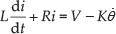
where J is the moment of inertia of the rotor, τ_a is the torque applied to the shaft of the motor, R is the electrical resistance of the motor, and V is the voltage applied.

Assuming that the electrical time constant $L / R$ is small enough, the motor inductance L is approximated as 0 [15]; therefore, (7) can be rewritten as follows:

R i = V - K \dot{θ}

(8)

3.2. Wheels

Assuming there is acceptable friction between wheels and the contact surface, a free body diagram of the forces and torques applied to the wheels can be derived (see Fig. 3). Since a gearbox with a gear ratio of 50:1 is attached between the motor shaft and the wheel, the torque applied to the wheels is assumed to be 50 times the output torque from the motor:

Figure 3.

Free body diagram of the wheel

From Newton's second law, two new equations are obtained:

H_{f} - H = m_{W} \ddot{x}

(9)

r H_{f} - 50 τ_{a} = I_{W} \frac{\ddot{θ}}{50} = I_{W} \frac{\ddot{x}}{r}

(10)

where H is the force applied to the wheel by the chassis, and H_f is the friction force applied to the wheel by the surface contact. I_W is the moment of inertia of the wheel, and r is the wheel radius.

3.3. Inverted pendulum

The robot chassis is modelled as an inverted pendulum, whose base is attached to the wheels. A two-dimensional free body diagram of the robot chassis is depicted in Fig. 4, where m_C is the chassis mass and l is the length from the base of the pendulum to its centre of mass.

Figure 4.

Inverted pendulum free body diagram

Adding forces in the horizontal direction, the following equation is obtained:

2 H = m_{C} \ddot{x} - m_{C} l \ddot{ϕ} \cos ϕ - m_{C} l {\dot{ϕ}}^{2} \sin ϕ .

(11)

The moments about the centre of mass in the pendulum are summarised as follows:

(I_{C} + m l^{2}) \ddot{ϕ} - m_{C} g l \sin ϕ = m_{C} l \ddot{x} \cos ϕ .

(12)

It is possible to linearize both (11) and (12) by making the following approximations:

\begin{matrix} \sin ϕ \approx ϕ \\ \cos φ \approx 0 \\ ϕ^{2} \approx 0. \end{matrix}

Substituting these approximations into (11) and (12), the following equations are obtained:

2 H = m_{C} \ddot{x} - m_{C} l \ddot{ϕ}

(13)

(I_{C} + m l^{2}) \ddot{ϕ} - m_{C} g l ϕ = m_{C} l \ddot{x}

(14)

Figure 5.

Cascade control for the self-balancing vehicle

3.4. State space model

In order to test the controllers proposed in section 5, a state space model of the self-balancing vehicle was used to simulate the response of the system. Since the equations are linear, they can be written in the standard matrix form, as follows:

[\begin{matrix} \dot{x} \\ \ddot{x} \\ \dot{ϕ} \\ \ddot{ϕ} \end{matrix}] = A [\begin{matrix} x \\ \dot{x} \\ ϕ \\ \dot{ϕ} \end{matrix}] + B u;

(15)

y = [\begin{matrix} 1 & 0 & 0 & 0 \\ 0 & 0 & 1 & 0 \end{matrix}] [\begin{matrix} x \\ \dot{x} \\ ϕ \\ \dot{ϕ} \end{matrix}] + [\begin{matrix} 0 \\ 0 \end{matrix}] u

(16)

where the pitch angle φ and the position x are the outputs of the system, and the voltage applied to the motors V is the input u.

Element values for matrices A and B were obtained by substituting i from (8) into (6), and then substituting τ_a from (6) into (10). Then, H_f from (10) was substituted into (9), and, finally, force H from (9) into (13).

The resulting matrices for the state space model are:

A = [\begin{matrix} 0 & 1 & 0 & 0 \\ 0 & \frac{2 \cdot 50^{2} K^{2}}{r^{2} R W_{1}} & \frac{- g m_{C}^{2} l^{2}}{W_{1} (I_{C} + m_{C} l^{2})} & 0 \\ 0 & 0 & 0 & 1 \\ 0 & \frac{2 \cdot 50^{2} K^{2}}{r^{2} R W_{2}} & \frac{- g m_{C}^{2} l^{2}}{W_{2} ((I_{C} + m_{C} l^{2}) + g W_{1})} & 0 \end{matrix}]; B = [\begin{matrix} 0 \\ \frac{- 100 K}{r R W_{1}} \\ 0 \\ \frac{- 100 K}{r R W_{2}} \end{matrix}]

(17)

where W₁ and W₂ become:

\begin{matrix} W_{1} = 2 (\frac{- 50^{2} J + I_{W}}{r^{2}} - m_{W}) - m_{C} + \frac{m_{C}^{2} l^{2}}{I_{C} + m_{C} l^{2}} \\ W_{2} = W_{1} (\frac{I_{C}}{m_{C} l} + l) \end{matrix}

Estimated values attributed to the robot used in experimental tests were obtained by measuring the weights and dimensions of the chassis, wheels, and motors of the robot. The obtained values are:

K = 0.24 N m / A,

m_{C} = 3.0 K g,

l = 0.1 m,

r = 0.04825 m,

I_{c} = 0.0125 K g m^{2},

g = 9.81 m / s^{2},

R = 3.0 Ω,

m_{W} = 0.113 K g,

I_{W} = 0.0001548 K g m^{2},

J = 0.0003.

4. Cascade Control

A cascade control is designed to increase the control performance when the system can be considered as two processes in series. The increase in performance is a consequence of the fact that the disturbances in the secondary process are not measured until they have affected the output of the primary process [16]. In a self-balancing vehicle, the linear velocity is strongly affected by the pitch angle. Therefore, the linear velocity could be considered as the primary process and the pitch angle as the secondary process. In Fig. 5, the cascade control of the self-balancing vehicle is illustrated.

Odometry was used to locate the self-balancing vehicle in a Cartesian plane based on the angular velocity of the wheels. The required variables to obtain the linear and angular velocities are shown in Fig. 6. l is the length of the vehicle, as measured from the end of one wheel to the end of the other. v and ω are the linear and angular velocities of the vehicle, respectively.

Figure 6.

Motion equation variables

Assuming there is no slip between the wheels and the ground, the values for v and ω can be obtained from the angular velocities of the wheels ( ${\dot{θ}}_{R}$ and ${\dot{θ}}_{L}$ ) using the following equation [17]:

[\begin{matrix} v \\ ω \end{matrix}] = [\begin{matrix} \frac{r}{2} & \frac{r}{2} \\ \frac{r}{l} & - \frac{r}{l} \end{matrix}] [\begin{matrix} {\dot{θ}}_{R} \\ {\dot{θ}}_{L} \end{matrix}]

(18)

5. Control Design

The vehicle has to balance on its own. In other words, the vehicle has to keep from falling while moving on the ground. In order for the controller to keep balance, the pitch angle (the angle between the chassis and the vertical axis) needs to be reduced to zero. In order to maintain linear velocity control, the pitch controller must be able to change the set point to a value close to zero to keep balance, a positive value to move forward, and a negative value to move backward.

The controllers proposed for both the pitch angle control and the linear velocity control are PID. An extra controller was implemented for the angular velocity. Since the required action to change the orientation of the self-balancing vehicle has no impact on the actions of the main controllers (pitch angle and linear velocity), this extra controller can be added without introducing a significant disturbance.

The addition of this controller achieves the final configuration of the controllers, as shown in Fig. 7, where v_r is the linear velocity reference and ω_r is the angular velocity reference. The outputs of the self-balancing vehicle are the pitch angle φ, angular velocity of the left wheel ${\dot{θ}}_{L}$ , and angular velocity of the right wheel ${\dot{θ}}_{R}$ . The inputs of the vehicle are the voltage applied to the motor of the left wheel, V_L, and the voltage applied to the motor of the right wheel, V_R. Small oscillations introduced to the system by the self-balancing process are filtered out by passing the linear velocity signal through a low-pass filter. This leads to an improved measurement of the linear velocity.

Figure 7.

Diagram of the proposed controllers

6. Simulation

In order to adjust the gains of the pitch angle and linear velocity controllers, a simulation of the system was executed in Matlab^©. To accomplish this task, the model obtained in section 3.4 was used. Additionally, the behaviour of the controller was considered. The variables were sampled every 10 ms.

Fig. 8 shows the response of the pitch angle and the position using only a pitch angle controller. There is no cascade control in this simulation. The initial conditions for the state variables are [x ẋ φ φ̇]^T = [0 0 1.15° 0]^T. It can be seen that the pitch angle reached 0° after 0.5 seconds. Nevertheless, the position drifts from the zero reference. This behaviour was expected, since there is no control over the position or the linear velocity.

Figure 8.

Pitch angle (left) and position (right) response in simulation with only pitch angle control

Fig. 9 shows the response of the vehicle when the cascade control system is implemented in a second simulation. In this simulation, the linear velocity reference v_r was set to 0. The simulation shows that the pitch angle can be controlled as close as possible to $0 °$ , while the linear velocity reaches 0. Accordingly, the position of the vehicle remains constant after 4 s.

Figure 9.

Pitch angle (left) and position (right) response in simulation with pitch angle and velocity control

In Fig. 10, the response from another simulation is shown. Again, cascade control was implemented, but the linear velocity reference v_r was set to $0.1 m / s$ . The linear velocity reached the reference point in 0.5 s and stabilized after approximately 1 s. The position increases along with the linear velocity at $0.1$ metres per second. Finally, the voltage applied to the motors is also plotted. The voltage remains constant, as does the velocity ( $V_{R} = V_{L} \approx 0.5 V$ ). This means that the motors are powered so that they can move the vehicle.

Figure 10.

Pitch angle (top left), position (top right), linear velocity (bottom left) and input motor voltage (bottom right) response with pitch angle and velocity control

7. Motion Control

In mobile robotics, it is crucial to understand the behaviour of a given mechanical configuration in order to create control software for a particular piece of hardware [18].

Once the control is able to balance the mobile robot by controlling both the linear velocity and the angular velocity, it is possible to move the robot on a Cartesian plane. The kinematics of the self-balancing vehicle and those of a differential-drive robot are very similar.

7.1. Kinematics

The motion equations for the self-balancing vehicle are as follows:

[\begin{matrix} \dot{x} \\ \dot{y} \\ \dot{ψ} \end{matrix}] = [\begin{matrix} \cos ψ & 0 \\ \sin ψ & 0 \\ 0 & 1 \end{matrix}] [\begin{matrix} v \\ ω \end{matrix}]

(19)

where v is the linear velocity of the vehicle and ω is the angular velocity (both parameters were already obtained in 18). Variables $\dot{x}$ and $\dot{y}$ are the Cartesian velocities and ψ̇ is the velocity of the orientation angle of the vehicle.

In order to integrate equation 19, a modified Euler method was used [19]. This method is given as follows:

y_{n + 1} = y_{n} + h f (t_{n} + \frac{h}{2}, y_{n} + \frac{h}{2} f (t_{n}, y_{n}))

(20)

From (20), a discrete equation is obtained in order to determine the approximate position of the vehicle:

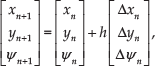
[\begin{matrix} x_{n + 1} \\ y_{n + 1} \\ ψ_{n + 1} \end{matrix}] = [\begin{matrix} x_{n} \\ y_{n} \\ ψ_{n} \end{matrix}] + h [\begin{matrix} Δ x_{n} \\ Δ y_{n} \\ Δ ψ_{n} \end{matrix}],

(21)

where h is the sampling interval of the variables’ acquisition using the information from the encoders located in the wheels. Considering the modified Euler method, vector velocity ${[\begin{matrix} Δ x_{n} & Δ y_{n} & Δ ψ_{n} \end{matrix}]}^{T}$ is evaluated as follows:

[\begin{matrix} Δ x_{n} \\ Δ y_{n} \\ Δ ψ_{n} \end{matrix}] = [\begin{matrix} v_{n} \cos (ψ_{n} + \frac{h}{2} ω_{n}) \\ v_{n} \sin (ψ_{n} + \frac{h}{2} ω_{n}) \\ ω_{n} \end{matrix}] .

(22)

As stated in section 6, interval h is equal to $10 m s$ for the self-balancing vehicle. It should be noted that a constant velocity is assumed for each time interval h.

7.2. Control design

The purpose of this control is to drive the robot to a desired position. This desired position is called reference position or reference posture (see Fig. 11). In order to obtain an error between the actual position and the reference position, the following equation is derived:

[\begin{matrix} e_{x} \\ e_{y} \\ e_{ψ} \end{matrix}] = [\begin{matrix} \cos ψ & \sin ψ & 0 \\ - \sin ψ & \cos ψ & 0 \\ 0 & 0 & 1 \end{matrix}] [\begin{matrix} x_{r} - x \\ y_{r} - y \\ ψ_{r} - ψ \end{matrix}] .

(23)

Figure 11.

Motion equation variables

Error e_x can be derived from a vector projection of unit vector u on a vector from the actual position towards the reference position. In a similar way, e_y is obtained from a vector projection of unit vector u on a vector from an orthogonal vector to a vector from the actual position towards the reference position (see Fig. 11).

e_{x} = | (x_{r} - x, y_{r} - y) | P r o j_{(x_{r} - x, y_{r} - y)} \vec{u}

(24)

e_{y} = | (x_{r} - x, y_{r} - y) | P r o j_{(y - y_{r}, x_{r} - x)} \vec{u}

(25)

The controller can be derived from observing error vectors in Fig. 11. The objective of this controller is to reduce the error vector ${[\begin{matrix} e_{x} & e_{y} & e_{ψ} \end{matrix}]}^{T}$ . In order to reduce e_x, the linear velocity v should be changed proportionally to this error. To reduce e_y, the angular velocity ω should be changed proportionally to this error and multiplied by the sign of the linear velocity. To reduce e_ψ, again, ω should be proportional to this error. The following equation defines the control law for the self-balancing vehicle:

[\begin{matrix} v \\ ω \end{matrix}] = [\begin{matrix} k_{1} & 0 & 0 \\ 0 & - s i g n (v_{r}) k_{2} & k_{3} \end{matrix}] [\begin{matrix} e_{x} \\ e_{y} \\ e_{ψ} \end{matrix}],

(26)

where

k_{1} > 0, k_{2} > 0, k_{3} > 0.

8. Experiments and Results

In order to test the performance of the different controllers proposed in this work, several experiments were carried out. The main variables that define the state of the vehicle were plotted to show the behaviour of the controller.

Four experiments are described in the next subsections. In the first experiment, pitch and velocity control was implemented; at a given time, some disturbances were applied to the system. In the second experiment, pitch, velocity, and motion control was implemented, and a change in the centre of mass of the robot was introduced. In the third experiment, the robot was placed on an inclined surface while implementing pitch, velocity, and motion control. In the last experiment, the robot was placed in a flat surface with no inclination; the robot position set-point given to the motion control was changed at three given times.

8.1. Pitch angle and linear velocity control

In a first experiment, the self-balancing vehicle is controlled only by the cascade control system, using the controller described in Fig. 7. In other words, a controller is present for the linear velocity and for the angular velocity only. The set-points for each controlled variable were set to $v_{r} = 0.0 m / s$ and $ω_{r} = 0.0 r a d / s$ .

Pitch angle and position data were recorded for 20 seconds. Then, the collected data were plotted in Figures 12 and 13. Since angular velocity is not strongly affected by disturbances in the system, data related to this variable were not plotted.

In this experiment, the two disturbances D₁ and D₂ were introduced to the vehicle at $t_{1} = 4.75$ and $t_{2} = 16.2$ , respectively. The disturbances represented a slight push of the vehicle in both directions (forwards and backwards).

When the vehicle reaches a stable state, the pitch angle varies from $φ_{m i n} = - 0.377 °$ to $φ_{m a x} = 1.064 °$ . This means that the angle is kept in a $Δ φ = 1.441 °$ range. The maximum reached angle after D₁ is $6.97 °$ . The minimum reached angle after D₂ is $- 6.276 °$ (see Fig. 12).

From the plotted data, when the vehicle reaches a stable state, the position varies from $x_{m i n} = - 0.096$ m to $x_{m a x} = - 0.081$ m. This means that the position is kept in the range of $Δ x = 0.015$ m. The minimum reached position after D₁ is $- 0.208$ m. The maximum reached position after D₂ is $0.068$ (see Fig. 13).

Figure 12.

Pitch angle response with only pitch angle and linear velocity control

Figure 13.

Position response with only pitch angle and linear velocity control (no control on position)

8.2. Position control

A second experiment was carried out implementing position control defined by the control law from (26). Displacement along x is considered. In this experiment, x_r was set to $0.0$ m. Data were recorded for 50 seconds. Within this time interval, three events, E₁, E₂, and E₃, were executed. These events are defined as follows:

$E_{1} (t = 7.5 s)$ . Low weight was added to one side of the vehicle in order to change the centre of mass.

$E_{2} (t = 21 s)$ . Another low weight was added to the previous one.

$E_{3} (t = 37 s)$ . Both weights were detached from the vehicle.

Fig. 14 shows how the pitch angle of equilibrium changes when the centre of mass changes. The cascade control system compensates the change of the position of the centre of mass by changing the pitch angle of equilibrium. Before E₁ occurs, the mean pitch angle of equilibrium is approximately $0 °$ . After E₁ takes place, this angle changes by $- 1 °$ . Then, after E₂, this angle changes by $- 3 °$ . Finally, when the weights are detached (E₃), the angle of equilibrium goes back to $0 °$ .

Fig. 15 shows how the position of the vehicle is affected by the changes in the centre of mass. Once the centre of mass is changed, the position drifts away from the reference. Then, after the angle of equilibrium is reached, the error between the vehicle position and the reference is reduced. Approximately five seconds after each event, the position has reached a steady state.

Figure 14.

Pitch angle response with position control

Figure 15.

Position response with position control

8.3. Position control on an inclined surface

Another experiment was carried out implementing position control with the vehicle positioned on an inclined surface. In a similar way as in the previous experiment, x_r was set to 0cm. The vehicle successfully balanced itself while keeping its position. Data were recorded for 10 seconds in order to obtain the plots presented in this section.

The experiment was divided into three parts:

A. On a surface with a −3° inclination.

B. On a surface with a 10° inclination.

C. On a surface with a 20° inclination.

Fig. 16 shows the plot of a pitch angle versus the time. The data collected from the experiment revealed that the pitch angle of equilibrium augments as the slope increases. During the first part of the experiment, the pitch angle of equilibrium is approximately $1.5 °$ and varies from $0.156 °$ to $2.713 °$ . During the second part, the pitch angle of equilibrium is approximately $- 6.5 °$ and varies from $- 8.084 °$ to $- 4.753 °$ . During the third part, the pitch angle of equilibrium is approximately $- 9.5 °$ and varies from $- 11.753 °$ to $- 7.346 °$ .

Fig. 17 shows the plot of the voltage applied to the motors. The mean voltage for each part of the experiment was recorded. The mean value of the voltage during the first part of the experiment is $- 0.39 V$ . During the second part, the mean value is $1.24 V$ . Finally, during the third part, the mean value is $1.59 V$ .

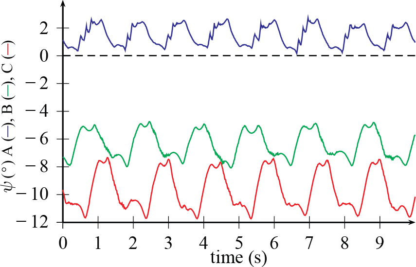
Fig. 18 shows the plot of the position of the vehicle. The obtained data show that the amplitude of the position increases when the slope of the surface is increased. During the first part, the position varies from $- 0.858 c m$ to $1.022 c m$ . During the second part, the position varies from $- 1.691 c m$ to $1.62 c m$ . Finally, during the third part, the position varies from $- 2.362 c m$ to $1.933 c m$ .

Figure 16.

Pitch angle on an inclined surface

Figure 17.

Action response on an inclined surface

Figure 18.

Position response on an inclined surface

8.4. Motion control

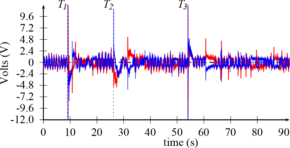
The motion control law proposed in section 7.2 was tested with a different experiment. Three reference positions, also called target positions, were set while recording the response of the vehicle to achieve these targets on a flat surface with no inclination. The following targets were defined:

T₁. At time $t_{1} = 9 s$ , ${[\begin{matrix} x_{r} & y_{r} & ψ_{r} \end{matrix}]}^{T} = {[\begin{matrix} 20 c m & 20 c m & 0 ° \end{matrix}]}^{T}$ .

T₂. At time $t_{1} = 26.2 s$ , ${[\begin{matrix} x_{r} & y_{r} & ψ_{r} \end{matrix}]}^{T} = {[\begin{matrix} 20 c m & - 20 c m & 0 ° \end{matrix}]}^{T}$ .

T₃. At time $t_{1} = 54 s$ , ${[\begin{matrix} x_{r} & y_{r} & ψ_{r} \end{matrix}]}^{T} = {[\begin{matrix} 0 c m & 0 c m & 0 ° \end{matrix}]}^{T}$ .

Before T₁, the target position is already set to ${[\begin{matrix} 0 c m & 0 c m & 0 ° \end{matrix}]}^{T}$ .

Fig. 19 shows the path that the vehicle follows to reach the desired targets. When the vehicle goes to T₁, it moves in the forward direction. The vehicle goes forwards again to reach T₂. Finally, when trying to reach T₃, the vehicle moves backwards. This behaviour occurs because of the initial orientation of the vehicle, which tries to take the shortest path; notice that the vehicle can always move in two directions (forwards or backwards). However, it will only move in the direction that is best oriented towards the target position.

In Fig.20, the actual position variables ${[\begin{matrix} x & y & ψ \end{matrix}]}^{T}$ are plotted against time t. It can be seen that after T₁ is set, the vehicle takes approximately $3 s$ to reach the desired target position. Nevertheless, the vehicle never reaches the exact position. The error obtained just before T₂ is set is ${[\begin{matrix} x_{r} - x & y_{r} - y & ψ_{r} - ψ \end{matrix}]}^{T} = {[\begin{matrix} - 0.11 c m & 1.014 c m & 0.859 ° \end{matrix}]}^{T}$ .

Fig. 21 shows the variations in the pitch angle when the vehicle tries to balance while going from one target to another. Finally, in Fig. 22, the voltage applied to the motors is plotted. It can be seen that, most of the time, the voltage is kept in a range not greater than $2.4 V$ . As expected, peaks of $12 V$ are produced when the target position is changed.

Figure 19.

Position response with motion control

Figure 20.

Position response with motion control

Figure 21.

Pitch angle response with motion control

Figure 22.

Input voltage applied to motors with motion control

9. Conclusions

The cascade controller proposed in this work is capable of successfully keeping the self-balancing vehicle from falling. The pitch angle can be kept under $1 °$ from the equilibrium position when no disturbances are introduced.

The addition of control for the linear velocity using motor encoders leads to a more stable system compared to one that does not implement these sensors.

Despite the fact that the proposed controller is based on a linear model, it can handle slight changes in the dynamics of the system. Two of the changes tested here have been the change of the centre of mass and the change in the slope of an inclined surface.

The motion control implemented in this work was able to drive the vehicle with an error of approximately $1 c m$ with respect to the desired position.

References

Azhar

M. Abdullah Bin

Hassan

Rahim

, Pid control behavior and sensor filtering for a self balancing personal vehicle. In Robotics and Artificial Intelligence (ICRAI), 2012 International Conference on, pages 7–10, Oct 2012.

Silva

Felipe Oliveira e

de Carvalho Ferreira

Luis Henrique

. Design and implementation of a pid control system for a coaxial two-wheeled mobile robot. In Industrial Electronics (ISIE), 2013 IEEE International Symposium on, pages 1–6, May 2013.

Unluturk

Aydogdu

Guner

, Design and pid control of two wheeled autonomous balance robot. In Electronics, Computer and Computation (ICECCO), 2013 International Conference on, pages 260–264, Nov 2013.

Liptak

B.G.

, Instrument Engineers' Handbook, Fourth Edition, Volume Two: Process Control and Optimization. Instrument Engineers' Handbook. CRC Press, 2005.

Stilman

Olson

Gloss

, Golem krang: Dynamically stable humanoid robot for mobile manipulation. In Robotics and Automation (ICRA), 2010 IEEE International Conference on, pages 3304–3309, May 2010.

Pratama

Derry

Binugroho

Eko Henfri

Ardilla

Fernando

. Movement control of two wheels balancing robot using cascaded pid controller. International Electronics Symposium (IES), 2015.

Alfaro

V.M.

Vilanova

Arrieta

, Two-degree-of-freedom pi/pid tuning approach for smooth control on cascade control systems. In Decision and Control, 2008. CDC 2008. 47th IEEE Conference on, pages 5680–5685, Dec 2008.

Majczak

Wawrzynski

, Comparison of two efficient control strategies for two-wheeled balancing robot. In Methods and Models in Automation and Robotics (MMAR), 2015 20th International Conference on, pages 744–749, Aug 2015.

Kumbasar

Hagras

, A type-2 fuzzy cascade control architecture for mobile robots. In Systems, Man, and Cybernetics (SMC), 2013 IEEE International Conference on, pages 3226–3231, Oct 2013.

10.

Perez

Milanes

Onieva

, Cascade architecture for lateral control in autonomous vehicles. Intelligent Transportation Systems, IEEE Transactions on, 12(1):73–82, March 2011.

11.

Sayidmarie

O.K.

Tokhi

M.O.

Agouri

S.A.

, Impact of dynamically moving payload on two wheeled robot stability. In Methods and Models in Automation and Robotics (MMAR), 2014 19th International Conference On, pages 915–920, Sept 2014.

12.

Sayidmarie

O.K.

Tokhi

M.O.

Agouri

S.A.

, Real-time validation of a novel two-wheeled robot with a dynamically moving payload. In Robot and Human Interactive Communication, 2014 RO-MAN: The 23rd IEEE International Symposium on, pages 102–105, Aug 2014.

13.

Sung-Kwun Oh Jang

Han-Jong

Pedrycz

Witold

. A comparative experimental study of type-1/type-2 fuzzy cascade controller based on genetic algorithms and particle swarm optimization. Expert Syst. Appl., 38(9):11217–11229, September 2011.

14.

Kumbasar

Tufan

Hagras

Hani

. Big bang-big crunch optimization based interval type-2 fuzzy pid cascade controller design strategy. Inf. Sci., 282:277–295, October 2014.

15.

Davies

Schmitz

T.L.

, System Dynamics for Mechanical Engineers. SpringerLink: Bücher. Springer New York, 2014.

16.

Erickson

K.T.

Hedrick

J.L.

, Plant-Wide Process Control. Wiley Series in Chemical Engineering. Wiley, 1999.

17.

Siciliano

Khatib

, Springer Handbook of Robotics. Gale virtual reference library. Springer, 2008.

18.

Siegwart

Nourbakhsh

I.R.

Scaramuzza

, Introduction to Autonomous Mobile Robots. Intelligent robotics and autonomous agents. MIT Press, 2011.

19.

Hassani

, Mathematical Methods Using Mathematica: For Students of Physics and Related Fields. Undergraduate Texts in Contemporary Physics. Springer, 2003.

Velocity and Motion Control of a Self-Balancing Vehicle Based on a Cascade Control Strategy