Sage Journals: Discover world-class research

Abstract

Two-wheeled self-balancing vehicle system is a kind of naturally unstable underactuated system with high-rank unstable multivariable strongly coupling complicated dynamic nonlinear property. Nonlinear dynamics modeling and simulation, as a basis of two-wheeled self-balancing vehicle dynamics research, has the guiding effect for system design of the project demonstration and design phase. Dynamics model of the two-wheeled self-balancing vehicle is established by importing a TSi ProPac package to the Mathematica software (version 8.0), which analyzes the stability and calculates the Lyapunov exponents of the system. The relationship between external force and stability of the system is analyzed by the phase trajectory. Proportional–integral–derivative control is added to the system in order to improve the stability of the two-wheeled self-balancing vehicle. From the research, Lyapunov exponent can be used to research the stability of hyperchaos system. The stability of the two-wheeled self-balancing vehicle is better by inputting the proportional–integral–derivative control. The Lyapunov exponent and phase trajectory can help us analyze the stability of a system better and lay the foundation for the analysis and control of the two-wheeled self-balancing vehicle system.

Keywords

Two-wheeled self-balancing vehicle stability Lyapunov exponent phase trajectory PID

Introduction

In recent years, two-wheeled self-balancing vehicle is widely used for its advantages such as energy saving, environmental protection, simple structure, flexible operation, and so on. The research has a strong theoretical significance and practical value. In 1986, Yamato Gaoqiao, professor of Tokyo Electric Communication University, first designed the mobile robot of double coaxial and self-standing.¹ In 2002, the first two-wheeled self-balancing vehicle Segway human transporter (HT) was produced.² Now, a variety of standing and sitting vertical two-wheeled self-balancing vehicles have been developed. Two-wheeled self-balancing vehicles can maintain dynamics balance, but they also have an unstable dynamics characteristic.³ As a result, the stability of the two-wheeled self-balancing vehicles is the key factor to be considered in the research and design.^4,5 At present, the research on the two-wheeled self-balancing vehicles mainly focused on the design and control of stability. A variety of control algorithms have been developed. The Segway personal transporter used redundant control algorithm,^6,7 the HT vehicle of Camosun College used the fuzzy control algorithm,⁸ the two-wheeled vehicle of Adelaide University used proportional-derivative (PD) control method, and “free mover” in China University of Science and Technology used proportional–integral–derivative (PID) control algorithm.⁹ These algorithms can ensure dynamics stability of two-wheeled self-balancing vehicles and users can flexibly operate through a simple training. But as a nonlinear system, two-wheeled self-balancing vehicles have many characteristics, such as multivariable,¹⁰ strong coupling,¹¹ and nonholonomic constraints and parameter uncertainty.^12,13 Analysis and study of the dynamics characteristics of the two-wheeled vehicles are very complicated. At present, the research in this area is relatively few. It has become a focus of how to understand its intrinsic characteristics by the simple external structure of the two-wheeled self-balancing vehicle.

In this article, a dynamics modeling method with software package ProPac TSi is used and a PID controller is designed for its simple structure and other advantages. Also, a method based on Lyapunov exponent¹⁴ is used to analyze the stability of the vehicle system.¹⁵ And Lyapunov exponent, which is related to system stability, is an average of the contraction and expansion characteristics of the orbits in different directions in the phase space. Then, according to the system phase trajectory attractor types, influence of different PID coefficients on the stability of the system is analyzed. The control effectiveness is validated through the numerical simulation, and the results demonstrate that PID controller can effectively ensure stability and provide robust self-balancing control.

The rest of this article is organized as follows. Section “Methodology” describes the methodology of the proposed vehicle including dynamics modeling and calculation of Lyapunov exponents. Section “Simulation” shows the simulation results of Lyapunov exponents and PID controller. Finally, some conclusions are presented in the last section.

Methodology

Dynamics modeling

Two-wheeled self-balancing vehicle system mainly consists of two parts, namely, the body and the pendulum bar, and the pendulum bar is mainly used to control the motion of the vehicle.¹⁶ Two-wheeled self-balancing vehicle has three degrees of freedom, that is, rotation of pendulum bar around wheel set, translational motion, and turning motion of body in the horizontal plane. We selected angle Φ ¹⁷ between pendulum bar and vertical direction, body turning angle θ, and body translational displacement x as the generalized coordinates, corresponding to the pseudo velocity, respectively, w_y , w_z , and v_x .

In order to facilitate the analysis, some assumptions are made as follows:

The body and pendulum bar are regarded as rigid body.

The influence of different users’ weight and height is reflected on body weight and pendulum bar’s center of gravity.

Wheels only scroll without sliding and sideslip.

Ignoring air resistance and other tiny friction.

The working principle of two-wheeled self-balancing vehicle is similar to that of an inverted pendulum.^18,19 In order to facilitate the modeling, the two-wheeled vehicles can be reduced to a physical model as shown in Figure 1.

Figure 1.

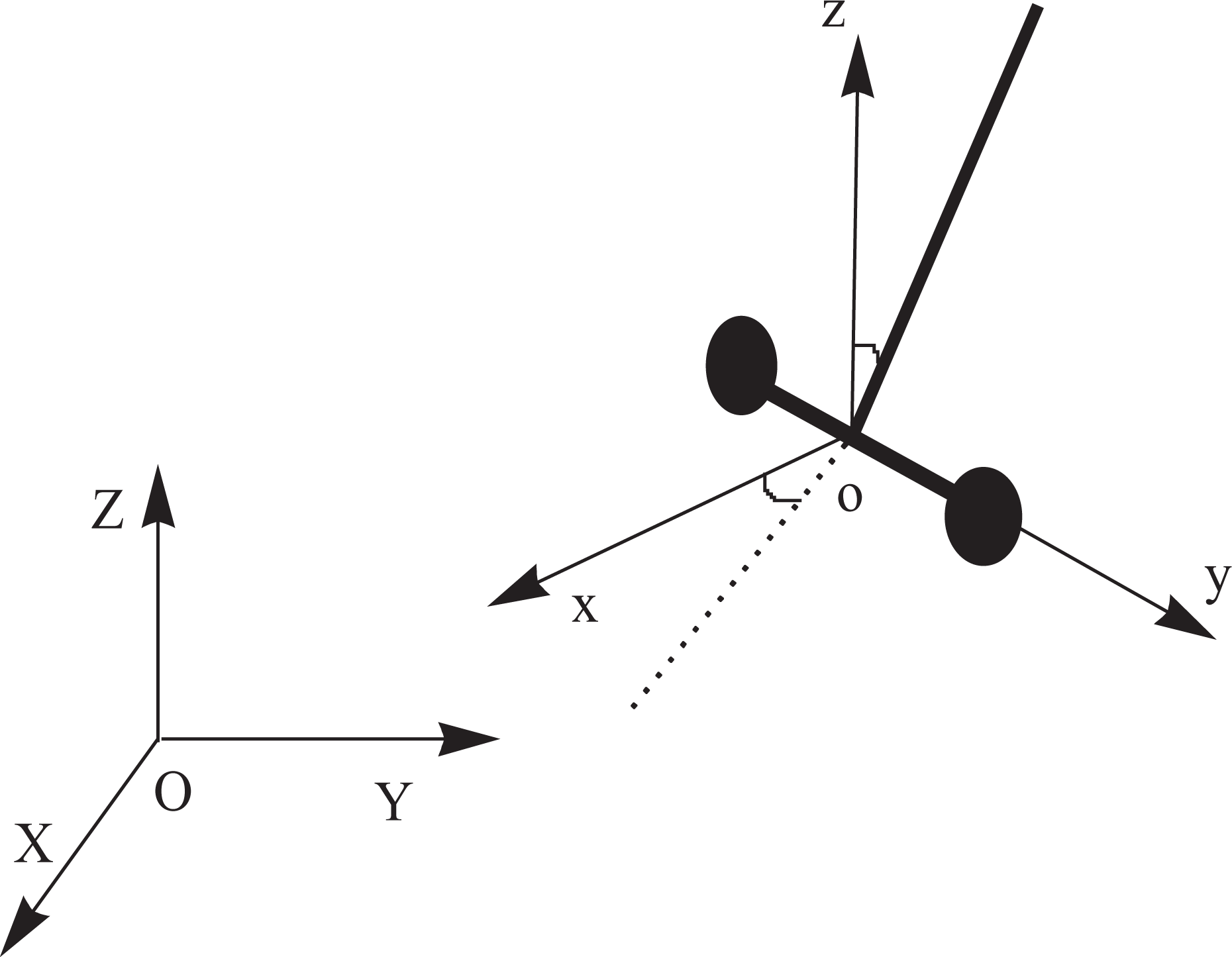
Simplified model of two-wheeled vehicle.

In Figure 1, the position and orientation of the two-wheeled vehicles are described by the coordinates of the three-dimensional coordinate system o-xyz fixed to the rigid body and the inertial reference frame O-XYZ. Then, import the ProPac TSi dynamics modeling software package into the Mathematica software, building dynamics modeling of the two-wheeled vehicle system, solving the equations of its kinematics and dynamics. The main parameters of the model are as follows:

m ₁: Sum of the mass of the vehicle body and the person

m ₂: Pendulum bar weight

g: Acceleration of gravity

a: Body and person’s centroid position

b: Pendulum bar height

c: Body width

F: Output force of motor

I ₁, I ₂: Inertia tensor of vehicle body and pendulum bar

The units of the aforementioned parameters are the international standard units. Through consulting data, we get its value.

The Euler–Poincare equation is used to establish the system model. The dynamics modeling process is as follows:

Step 1: Initialization

Define joint data

$r_{1} = {3}; q_{1} = {q, x, y}; p_{1} = {w z, v x, v y}$

$H_{1} = {{0, 0, 0}, {0, 0, 0}, {1, 0, 0}, {0, 1, 0}, {0, 0, 1}, {0, 0, 0}}$

$r_{2} = {1}; q_{2} = {f}; p_{2} = {w y}$

$H_{2} = {{0}, {1}, {0}, {0}, {0}, {0}}$

$JointLst = {{r_{1}, H_{1}, q_{1}, p_{1}}, {r_{2}, H_{2}, q_{2}, p_{2}}}$

Define body data

$cm1 = {0, 0, 0}; out1 = {{2, {0, 0, 0}}, {3, {0, c, 0}}, {4, {0, - c, 0}}}$

$I_{1} = {{J_{x x}, 0, J_{x z}}, {0, J_{y y}, 0}, {J_{x z}, 0, J_{z z}}}$

$cm2 = {0, 0, a}; out2 = {{5, {0, 0, b}}}$

$I_{2} = {{0, 0, 0}, {0, I_{y}, 0}, {0, 0, 0}}$

$BodyLst = {{cm1, out1, m1, I1}, {cm2, out2, m2, I2}}$

Define interconnection structure

$TreeLst = {{{1, 1}, {2, 2}}}$

Define potential energy

g = gc

PE = 0

Q = {0, F₁, 0, T₂}

Step 2: Dynamics modeling

${V, X, H, M, Csys, Fsys, psys, qsys} = CreateModel [JointLst, BodyLst, TreeLst, g, 0, Q]$

$quations = MakeODEs [p, q, V, M, Csys, Fsys, t]$

Step 3: Parameterization

END

The kinematics and dynamics equations are shown in the following equation²⁰

\begin{array}{l} \dot{q} = V (q) p \\ M (q) \dot{p} + C (p, q) p + F (p, q) = Q \end{array}

where q is the generalized coordinate vector and $q = {(θ, φ, x, y)}^{T}$ . p is the pseudo velocity vector and $p = {(w_{z}, w_{y}, v_{x}, v_{y})}^{T}$ . V(q), M(q), and C(q, p) are kinematics matrix, inertia matrix, and gyroscopic matrix, respectively.

F (p, q) is the viscous friction and gravity and Q is the external forces and moments. By establishing the model and numerical calculation, parameter matrixes of the above two equations are obtained as follows

M (q) = [\begin{matrix} A_{11} & 0 & A_{13} & 0 \\ 0 & A_{22} & 0 & A_{24} \\ A_{31} & 0 & A_{32} & 0 \\ 0 & A_{42} & 0 & 0 \end{matrix}]

where

$A_{11} = J_{z z} + a^{2} m_{2} sin {[φ]}^{2}$

$A_{13} = a m_{2} sin [φ]$

$A_{22} = m_{1} + m_{2} cos {[φ]}^{2} + m_{2} sin {[φ]}^{2}$

$A_{24} = a m_{2} cos [φ]$

$A_{31} = a m_{2} sin [φ]$

$A_{33} = m_{1} + m_{2}$

$A_{42} = a m_{2} cos [φ]$

\begin{matrix} F (p, q) = (\begin{matrix} 0 \\ - F \\ 0 \\ - a g m_{2} sin [φ] \end{matrix}) \\ C (p, q) = (\begin{matrix} C_{11} & C_{12} & C_{13} & C_{14} \\ C_{21} & 0 & C_{23} & C_{24} \\ 0 & C_{32} & 0 & C_{34} \\ C_{41} & C_{42} & C_{43} & C_{44} \end{matrix}) \end{matrix}

where

$C_{11} = a m_{2} v_{x} sin [φ]$

$C_{12} = - v_{y} (m_{1} + m_{2} cos {[φ]}^{2} + m_{2} sin {[φ]}^{2})$

$C_{13} = (m_{2} + m_{2}) v_{x}$

$C_{14} = 2 a^{2} m_{2} w_{z} cos [φ] sin [φ]$

$C_{21} = - a m_{2} w_{z} sin [φ]$

$C_{23} = - (m_{1} + m_{2}) w_{z}$

$C_{24} = - a m_{2} w_{y} sin [φ]$

$C_{32} = w_{z} (m_{1} + m_{2} cos {[φ]}^{2} + m_{2} sin {[φ]}^{2})$

$C_{34} = 2 a m_{2} w_{z} \cos [φ]$

$C_{41} = \frac{1}{2} (- a m_{2} v_{y} cos [φ] - 2 a^{2} m_{2} w_{z} cos [φ] sin [φ])$

$C_{42} = \frac{1}{2} a m_{2} w_{y} sin [φ]$

$C_{43} = - \frac{1}{2} a m_{2} w_{z} \cos [φ]$

$C_{44} = - \frac{1}{2} a m_{2} v_{x} sin [φ]$

J_zz is the moment of inertia around Z axis and I_y is the moment of inertia around the Y axis. From equation (1), the generalized coordinate vector q and the quasi-velocity vector p can be obtained as equations (2) and (3)

\dot{q} = V (q) p

\dot{p} = - M^{- 1} . (C s y s . p + F s y s)

Equations (2) and (3) are transformed into the form of the system state equation, that is, equation (4)

X = f (X)

where $X = {[q p]}^{T} = {(φ, θ, ψ, x, y, z, p, q, r, u, v, w)}^{T}$ is the state quantity.

Calculation of Lyapunov exponents

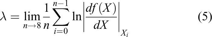
Lyapunov exponent, which is calculated as equation (5), is related to the initial moments of the system’s motion track with two infinitely close points that are separated by time. It is an average of the contraction and expansion characteristics of the orbits in different directions in the phase space.²¹ N dimensional system has n Lyapunov exponents, and each Lyapunov exponent can be regarded as the phase space in all directions of motion relative to the local deformation of the average

λ = \lim_{n \to 8} \frac{1}{n} {\sum_{i = 0}^{n - 1} \ln | \frac{d f (X)}{d X} |}_{X_{i}}

This article is based on the dynamics equation method to calculate the Lyapunov exponent. Let W denotes the tangent vector of the system track, and it can be obtained from equation (4), which can be represented as

\frac{d W}{d t} = J [X (t) W]

where X (t) is the solution of equation (4). J[ X ] is the Jacobian matrix of this equation.

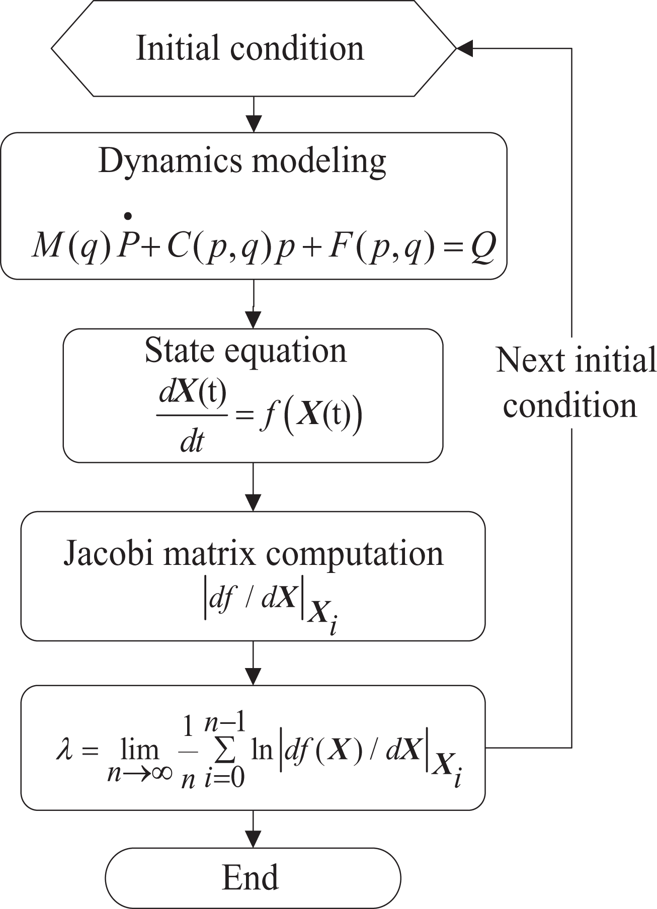
The sampling instant T is fixed at 0.1 s and the iterative value K is fixed at 100 in order to calculate the Lyapunov exponent. The initial condition of equation (6) is set as ${u_{1}^{(k - 1)}, u_{2}^{(k - 1)}, \dots u_{8}^{(k - 1)}}$ for the iteration of $k (k = 1, 2, \dots N)$ . The initial condition ${u_{1}^{(k - 1)}, u_{2}^{(k - 1)}, \dots u_{8}^{(k - 1)}}$ is transformed into ${w_{1}^{(k - 1)}, w_{2}^{(k - 1)}, \dots w_{8}^{(k - 1)}}$ through the T _s integral transformation. Then, ${w_{1}^{(k - 1)}, w_{2}^{(k - 1)}, \dots w_{8}^{(k - 1)}}$ is transformed by GramSchm orthogonal and turns into the vector ${v_{1}^{(k - 1)}, v_{2}^{(k - 1)}, \dots v_{8}^{(k - 1)}}$ . Finally, the ultimate vector is obtained, that is, ${u_{1}^{k}, u_{2}^{k}, \dots u_{8}^{k}}$ . Repeat this process until the Lyapunov exponent reaches the maximum number of iterations N. The exponent obtained forms Lyapunov exponent spectrum. The calculation process is shown in Figure 2.

Figure 2.

Flowchart of Lyapunov exponent calculation.

This article is based on the Lyapunov exponent method to judge the stability of a two-wheeled vehicle system. When the Lyapunov exponents are greater than 0, the system is unstable or chaotic.^22,23 When the Lyapunov exponent is 0, the phase trajectory is periodic motion.²⁴ When the Lyapunov exponent of all states of the system is less than 0, the phase orbit of the system is attracted to a stable fixed point, and the whole system is stable.²⁵

Simulation

Simulation and analysis based on Lyapunov exponents

By means of symbolic computation software Mathematica, the dynamics equations of the system are programmed and simulated, and the Lyapunov exponent spectrum of each variable of the two-wheeled vehicle system is obtained. The vehicle system is an eight-dimensional system with four generalized coordinates and four pseudo speeds, and the Lyapunov exponent spectrums are also eight dimensional. The corresponding exponential spectra of the calculated variables are shown in Figure 3.

Figure 3.

Lyapunov exponent.

It can be seen from the exponential spectrum curve of the whole system that the Lyapunov exponent of three variables in the system is greater than 0. Therefore, the two-wheeled vehicle system is a super chaotic system,¹⁷ and its motion behavior is closely related to the initial condition and the movement behavior is extremely complex and difficult to predict.

Two-wheeled vehicle has unstable dynamics characteristics, and stability is influenced by three main factors, namely, system structure parameters, external forces and moments applied to the system and the initial conditions. Phase trajectory curve can be used to analyze the impact of the external forces and moments on the stability of the two-wheeled vehicle.

PID control is used in this article. We selected angle Φ between pendulum bar and vertical direction as control variables, and the expectation is set to 0.03sinΦ. By changing the proportionality coefficient K_p , integral coefficient K_i , and differential coefficient K_d and simulation, phase trajectory can be obtained as shown in Figure 4, and then we analyze the influence of the coefficients on the dynamics characteristics of the system. Three coefficients of PID are shown below figure 4(a), the same as figure 4(b), figure 4(c) and figure 4(d).

Figure 4.

Trajectory simulation.

Figure 4 shows phase trajectory simulation of two-wheeled self-balancing vehicle whose driving force is controlled by PID algorithm. According to the phase trajectory direction, we can see that the force applied in the two-wheeled self-balancing vehicle has great influences on the stability of the system. The trajectory of Figure 4(a) is more chaotic and disorder, and the system has a super chaotic attractor. Its appearance is closely related to the instability of the system. Under the force, the two-wheeled vehicle is more sensitive to initial conditions, and its motion behavior is more complex, which cannot meet the self-balance of two-wheeled vehicle. When reducing integral coefficient, the phase trajectory simulation diagram is shown as Figure 4(b), and its trajectory relative to Figure 4(a) is more clear. It shows that the integral coefficient has an influence on the stability of the system. When the coefficient decreases, the system tends to be stable, but the system is still chaotic. When integral coefficient is 0, the simulation is shown as Figure 4(c) and the trajectory is more clear. It displays system seems to have fixed point attractor, but there is a downward extension of the line. With the combination of practical and two-wheeled vehicle simulation results, two-wheeled vehicle is not up to predetermined requirements. Figure 4(d) is a phase trajectory simulation diagram when the proportional and differential coefficients based on Figure 4(c) are constantly adjusted. At this time, proportion coefficient is 3860 and differential coefficient is 1980. It can be seen under the control of PD, angle Φ between pendulum bar and vertical direction and the angular velocity of the pendulum bar can tend to the point near (0,0) point. Two-wheeled system can be approximated to reach the equilibrium state. Simulation results are similar under the conditions of changing the initial value. Here, we can have a more intuitive understanding of the motion state of the two-wheeled vehicle system through the simulation diagram of the state of two-wheel vehicle.

Simulation and analysis of PID control

The principle of self-balance can be simply understood that when the pendulum bar moves forward in the direction of tilt, two-wheeled vehicle should accelerate to avoid the pendulum bar down. The same way when the pendulum rod back tilt, two-wheeled vehicle decelerates. In this article, the angle of the pendulum bar forward is recorded as positive, and the backward tilt is negative. Now let the car in normal travel by different disturbance, in order to observe the degree and the time to restore the stability of the state.

First of all, let the two-wheeled vehicle is subjected to a forward tilt of the disturbance

w_{y} [0] = 0. 1 v_{x} [0] = 10 v_{y} [0] = 0 Φ [0] = 0. 5 x [0] = 0 y [0] = 0 θ [0] = 0 w_{z} [0] = 0

The diagrams of pendulum bar angle, angular velocity, two-wheeled vehicle translational velocity, and translational displacement with time variation are shown in Figure 5(a) to (d).

Figure 5.

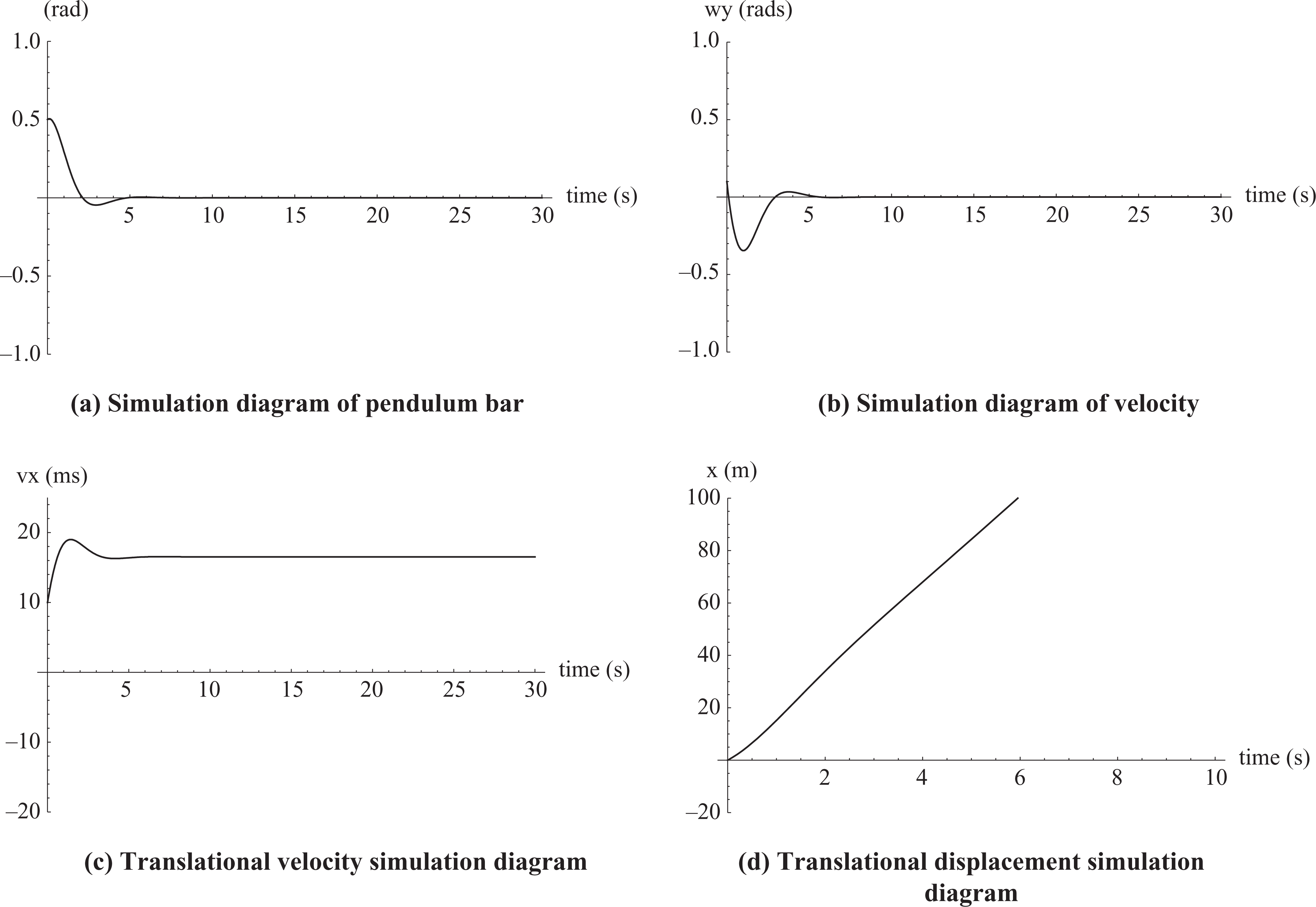
Two-wheeled vehicle acceleration state simulation diagram.

Figure 5(a) and 5(b) shows the curve of pendulum angle and angular velocity with time after the disturbance. It can be seen that the curve in the wave after a period of time can be restored to a stable state. Figure 5(c) shows that translational velocity can also tend to be stable after an acceleration fluctuation, and the vehicle runs smoothly with new speed. Figure 5(d) shows the displacement curve over time of the two-wheeled vehicle and the time change, from which we can work out the speed, and it is roughly consistent with Figure 5(c). Combined with practical experience, we can know that the control is generally in line with the requirements.

Then, let the two-wheeled vehicle is subjected to a backward tilt of the disturbance

w_{y} [0] = - 0. 1 v_{x} [0] = 10 v_{y} [0] = 0 Φ [0] = - 0. 5 x [0] = 0 y [0] = 0 θ [0] = 0 w_{z} [0] = 0

The diagrams of pendulum bar angle, angular velocity, two-wheeled vehicle translational velocity, and translational displacement with time variation are shown in Figure 6(a) to (d).

Figure 6.

Two-wheeled vehicle deceleration state simulation diagram.

Similar to the acceleration process, Figure 6(a) and (b) shows that the pendulum angle and angular velocity return to point near the zero after a period of fluctuations, that is, the pendulum bar approximates to maintain in the vertical direction and two-wheeled vehicle system achieves self-balance. Figure 6(c) shows that the translational velocity tends to be stable after reduction in volatility. Translational displacement increment speed shown in figure 6(d) is relatively slow compared with figure 5(d). Simulation results show that this article can achieve a series of operations such as start, stop, acceleration, deceleration, and disturbance self-recovery by driving force of PID control. The controlled angle range of pendulum bar is large, so it has a certain practical significance.

Conclusion

For two-wheeled self-balancing vehicle system, stability is the key factor to affect the performance characteristic. In this article, stability of two-wheeled self-balancing vehicle system is analyzed by the method of Lyapunov exponent. Phase trajectory is used to analyze influence on dynamics characteristics of the system. Researches show that Lyapunov exponent and system phase trajectory can help to understand the dynamics characteristics of the system. Finally, through numerical simulation, it is concluded that PID controller can effectively ensure stability and provide certain robustness for two-wheeled self-balancing vehicle system.

Footnotes

Acknowledgements

The authors thank the anonymous reviewers for helpful and insightful remarks. The authors also acknowledge helpful discussions with Professor Wu Qiong from Canada University of Manitoba on his guidance in Lyapunov exponent theory.

Declaration of conflicting interests

The author(s) declared no potential conflicts of interest with respect to the research, authorship, and/or publication of this article.

Funding

The author(s) disclosed receipt of the following financial support for the research, authorship, and/or publication of this article: This research is supported by the National Natural Science Foundation of China (51575283, 51405243, 51405241), the Natural Science Foundation of Jiangsu province (BK20130999), the open project (KDX1102) of Jiangsu Key Laboratory of Meteorological Observation and Information Processing, and Nanjing University of Information Science and Technology.GQ: Please confirm that the Funding and Conflict of Interest statements are accurate.]

References

Lam

Lee

Leung

FHF

. Fuzzy model reference control of wheeled mobile robots. In: The 27th annual conference of the IEEE industrial electronics society, 29 November–2 Decemeber 2009, Vol. 1. pp. 570–573. DOI: 10. 1109/IECON. 2001. 976547.

Sun

Zhou

. Design of two-wheel self-balanced electric vehicle based on MEMS. In: IEEE international conference on Nano/Micro engineered and molecular systems, China, 5–8 January 2009, pp. 143–146. DOI: 10. 1109/NEMS. 2009. 5068545.

Jung

Chung

. Calibration of kinematic parameters for two wheel differential mobile robots by using experimental heading errors. Int J Adv Robot Syst 2011; 8(5): 134–142. DOI: 10. 5772/50906. Available from: http://www.intechopen.com/journals/international_journal_of_advanced_robotic_systems/calibration_of_kinematic_parameters_for_two_wheel_differential_mobile_robots_by_using_experimental_h (accessed 18 March 2016).

Yang

. Student member, and Toshiyuki Murakami, senior member. Full-speed range self-balancing electric motorcycles without the handlebar. IEEE Trans Ind Electron 2016; 63: 1911–1915. DOI: 10. 1109/TIE. 2015. 2508925.

Antoska

Jovanović

Petrović

. Balance analysis of the mobile anthropomimetic robot under disturbances - ZMP approach. Int J Adv Robot Syst 2013; 10: 206. DOI: 10. 5772/56238.

Grasser

Darrigo

Colombi

. JOE: a mobile, inverted pendulum. IEEE Trans Ind Electron 2002; 49(1): 107–114. DOI: 10. 1109/41. 982254.

Lee

Jung

. Line tracking control of a two-wheeled mobile robot using visual feedback. Int J Adv Robot Syst 2013; 10: 177. DOI: 10. 5772/53729.

Ahmad

Siddique

Tokhi

(2012) Modular fuzzy logic controller for motion control of two-wheeled wheelchair. In: Dadios

(ed) Fuzzy logic - controls, concepts, theories and applications. InTech, DOI: 10. 5772/37584. http://www.intechopen.com/books/fuzzy-logic-controls-concepts-theories-and-applications/modular-fuzzy-logic-control-for-two-wheeled-wheelchair-motion-control (accessed 18 March 2016).

Study on self balance control system. Changsha: University of Science & Technology China, 2004. DOI: 10. 7666/d. y615623.

10.

Son

Anh

HPH

. Adaptive backstepping self-balancing control of a two-wheel electric scooter. Int J Adv Robot Syst 2014; 11: 165. DOI: 10. 5772/59100.

11.

Kausar

Stol

Patel

. The effect of terrain inclination on performance and the stability region of two-wheeled mobile robots. Int J Adv Robot Syst 2012; 9: 218. DOI: 10. 5772/52894.

12.

Gómez

Arribas

Sánchez

. Optimal control based on CACM-RL in a two-wheeled inverted pendulum. Int J Adv Robot Syst 2012; 9: 235. DOI: 10. 5772/54658.

13.

Azizi

Houshangi

. Mobile robot position determination. In: Topalov

(ed) Recent advances in mobile robotics. InTech, DOI: 10. 5772/26820. http://www.intechopen.com/books/recent-advances-in-mobile-robotics/mobile-robot-position-determination (accessed 8 April 2016).

14.

Luo

Liu

Che

. LMF algorithm based on hyper-chaos for the solving of forward displacement in a parallel robot mechanism. Int J Adv Robot Syst 2013; 10: 31. DOI: 10. 5772/54817.

15.

Sun

. Stability analysis via the concept of Lyapunov exponents: a case study in optimal controlled biped standing. Int J Control 2012; 85(12): 1952–1966. DOI: 10. 1080/00207179. 2012. 713985.

16.

Boucher

Sanchez

(2009) Mobile wheeled robot with step climbing capabilities. In: Chen

(ed) Mobile Robots - State of the Art in Land, Sea, Air, and Collaborative Missions. InTech. DOI: 10. 5772/6988. http://www.intechopen.com/books/mobile-robots-state-of-the-art-in-land-sea-air-and-collaborative-missions/mobile-wheeled-robot-with-step-climbing-capabilities (accessed 8 April 2016).

17.

Liu

HHS

Pang

GKH

. Accelerometer for mobile robot positioning. IEEE Trans Ind Appl 2001; 3: 812–819. DOI: 10. 1109/28. 924763.

18.

Wenjun

Kang

Zhao

. Speed and orientation control of a two-coaxial-wheeled inverted pendulum. In: Proceedings of the 32nd Chinese Control Conference, China, 26–28 July 2013.

19.

Nawawi

(2010) Real-time control system for a two-wheeled inverted pendulum mobile robot. In: Fuerstner

(ed) Advanced Knowledge Application in Practice. InTech. DOI: 10. 5772/10362. http://www.intechopen.com/books/advanced-knowledge-application-in-practice/real-time-control-system-for-a-two-wheeled-inverted-pendulum-mobile-robot- (accessed 8 April 2016).

20.

Xiong

. Robot technology foundation. Wuhan: Huazhong University of Science and Technology press, 2014.

21.

Gilat

Aboudi

. Parametric stability of non-linearly elastic composite plates by Lyapunov exponents. J Sound Vib 2013; 235(4): 627–637. DOI: 10.1006/jsvi.2000.2936.

22.

Luo

Liu

Che

. Mathematical programming method based on chaos anti-control for the solution of forward displacement of parallel robot mechanisms. Int J Adv Robot Syst 2013; 10: 32. DOI: 10. 5772/54818.

23.

Zang

Iqbal

Zhu

. Applications of chaotic dynamics in robotics. Int J Adv Robot Syst 2016; 13: 60. DOI: 10. 5772/62796.

24.