
Abstract
This paper presents and discusses the results of an ongoing R&D project aiming to design and build a fully automated prototype of a specialized spherical robotic welding system for repairing hydraulic turbine surfaces eroded by cavitation pitting and/or cracks produced by cyclic loading. The system has an embedded vision sensor built to acquire range images by laser scanning over the blade's surface and produce 3D models to locate the damaged spots to be registered in a 3D coordinate system into the robot controller, enabling the robot to repair the flaws automatically by welding in layers. The paper is focused on the robot kinematic model and describes an iterative algorithm to process the inverse kinematics with only five degrees-of-freedom. The algorithm makes use of data collected from a vision sensor to ensure that the welding gun axis is perpendicular to the blade's surface. Besides this, it proposes a modelling and optimization mathematical routine for more efficient robot calibration, which can be used with any type of robot. This robot calibration optimization scheme finds the optimal error parameter vector based on the condition number of the manipulator transformation composed from the partial derivatives of the error parameters. Experimental results proved both the iterative algorithm to perform the inverse kinematics and the technique to optimize robot calibration to be very efficient.
1. Introduction
A consolidated process for repairing the blade surface of hydraulic turbines eroded by cavitation or damaged by fatigue cracks is the recovery of flaws using electric arc welding [1, 2, 3]. The welding process is performed manually after visual inspection of the blade's surface, which requires a turbine halt. These are very unfavourable conditions for human labour, with air temperatures around 40° C and 99% relative air humidity for dozens of hours.
The prototype constructed is a specialized robotic welding system for repairing damage on the surface of hydraulic turbine blades eroded by cavitation and/or fatigue cracks under cyclic loading by welding in layers, reducing risks and increasing the efficiency of the repairing process. The robot is designed to improve the quality of the cavitation and/or fatigue damage repair, reducing the incidence of welding defects, welding material consumption, repairing time and overall repair costs. In addition, the proposed technology is expected to remove welding personnel from a harsh environment, achieve a better blade surface profile and improve welding consistency.
A robot designed with those requirements must have the ability to weld within a large range of torch orientation angles; it has to be light, small, accurate and resistant to loads from any direction on its wrist; rigid to deflections and with the potential to be fixed at any position. Some of those characteristics have opposite effects, suggesting that some of them have to be compensated by the others. Nonetheless, although a few dedicated robots have already been constructed for this type of task [4, 5, 6], this robot features improvements made to the previous ones, since it was designed to be fully automated, with minimal intervention by human operators. Additionally, this robot is capable of operating in conditions comprising large distances between blades, since the turbines in which it is to operate are 8 m in diameter and there is at least 500 mm between blades [7, 8, 9].
It is generally accepted that manipulators designed for dexterity and kinematic models’ simplicity must have at least six degrees-of-freedom (d.o.f.). However, it was decided that this robot's dexterity could be limited to five d.o.f. in order to reduce weight and size and to increase portability. This solution can be justified considering that the welding torch does not need three orientation angles within the 3D space, since the torch has a cylindrical symmetry.
It is well known that welding tasks are generally performed with a quasi-constant torch orientation during long displacements when welding. Thus, the robot can track a seam for welding the beads with a small variation in one of its Euler angles, mostly rotation around the torch symmetry axis. Several approaches for finding inverse kinematic solutions for a five-d.o.f. serial manipulator have been published in the past few years [10, 11, 12, 13, 14], making use of either analytical or numerical methods, normally specific to a certain robot model or topology.
Analytical solutions for the inverse kinematics for high-degree-of-freedom robots are very difficult or impossible. A complete analytical formulation for the inverse kinematics of the five-d.o.f. Pioneer 2 robotic arm (P2Arm) was presented in [10], but the correct solution could only be found after testing some partial solution alternatives. Some of the former authors [11] proposed a different analytical solution for the same robot but using some geometrical restriction during operation for tracking a given trajectory, while keeping the orientation of one axis in the end-effector frame. However, different partial solutions had still to be checked before the correct solution was found. More recently, it was presented in [13] an analysis of the inverse kinematics of a five-d.o.f. robot, the Mitsubishi Melfa RV- 2AJ industrial robot, aiming at controlling the z-axis position only.
Other authors [14] presented a generalized solution for the five-d.o.f. revolute joint variables of a machine comprising 2-links and a spade-like three-d.o.f. end-effector obtained by solving a set of algebraic equations emerging from series of transformation matrices.
An iterative approach can be found in [15] for solving inverse kinematics by adding a virtual joint to the five-d.o.f. robot, expressing all joints by one variable and applying the one-dimensional iterative Newton-Raphson method to minimize the tip-position error.
In [12], an iterative algorithm was proposed for a five-d.o.f. welding robot with a wrist offset. The algorithm showed good results when the position and three orientation angles were given and tracks were performed, keeping that orientation constant.
The algorithm proposed here for our spherical robot, with no wrist offsets but the inclusion of a shoulder, requires a torch orientation vector, expressed only from two angles, as a 3D vector parallel to the torch symmetry axis assigned to every track point.
Other than the inverse kinematics problem, one very important procedure when building a complex robot from scratch is to perform a full robot calibration routine to assure that the kinematic model corresponds to the actual robot, since there is no previous nominal model. As with every robot, every time it is necessary to disassemble parts of that robot, the calibration procedure has to be re-executed. Once a robot has been completely calibrated, it is not necessary to recalibrate all the model parameters but only the ones related to the link that has been disassembled. For example, if a torch is to be changed or disassembled, it is necessary to calibrate only the torch parameters. Another important issue in our robot is that the vision system may be considered as another link belonging to the robot's kinematic chain, since all measurements have to be assigned to the robot base coordinate system.
Our robot can operate with online or offline programming modes. Every time the vision system is used to generate a map and transmit point coordinates to the robot controller, it works in an offline programming mode. However, one of the obstacles that makes the viability of offline programming difficult is the poor accuracy of robot static positioning, turning robot calibration into an important procedure.
During the past few decades many different robot calibration methods have been published. The large majority of them compensate for position errors in the kinematic model [16, 17, 18] and few are considered modeless methods that use mathematical regression modelling of the errors or neural networks, but with the disadvantage of needing a large number of sample measurements [19, 20, 21]. Currently, robot calibration is still an active area of research [22].
The robot calibration optimization method presented in this article comprises kinematic parameter modelling, since the control system is open and easily changed. An important contribution of this article is to propose a method to define which geometric parameters have to be included in the model and, more importantly, to improve the mathematical conditioning of the system. The results of the application of this optimization technique are to reduce the number of measurement points and to improve the positional accuracy compared to a non-optimized calibration model. There are no works presented to date showing results of a method like this one with experimental verification.
This article presents initially and briefly, in Sections 2 and 3, the entire robotic system and its kinematic model. Section 4 presents the iterative algorithm developed to perform the inverse kinematics, making use of data collected from a vision sensor to ensure that the welding gun's axis is perpendicular to the blade surface and to collect the results of point tracking. In Section 5, a brief revision of robot calibration theory is discussed. Section 6 proposes and discusses the mathematical routine to determine the optimal parameter set to be identified by the robot calibration process, based on the analysis of the condition number of the manipulator transformation partial derivatives of the error parameters. Section 7 presents experimental results and proves the success of the solutions.
2. Robot Characteristics
The robotic system prototype constructed has a spherical topology with five d.o.f., a pan-tilt wrist, electric stepper motors, rotary and linear actuators. The robot arm carries an embedded vision sensor for acquiring range images and modelling 3D structured surface maps. The maps are used to plan welding trajectories in 3D coordinates automatically, according to the welding strategy on the surface blade region to be welded. The measurement system is implemented via a mini-PC that is embedded in the system. The robot controller and welding controller systems are built on a reconfigurable architecture based on FPGA (Field Programmable Gate Arrays). The welding process type is the GMAW (Gas Metal Arc Welding), with a pulsed arc welding machine and tubular metal cored electrodes. The robot was designed to have easy assembly and fixation on the blades (either belts or magnetic paddles), high rigidity mechanics and trouble-free operation. Portability, low cost, lightweight, good repeatability and high positioning accuracy are features of the resulting robot [8].
2.1. Robot prototype
The robot constructed weights 30kg, has a spherical topology and a 2.0m outer diameter workspace with dimensions of 30 × 25 × 60–100cm without the welding torch. Figure 1 shows the constructed system.
The robot was designed to embody an integrated control system for managing several tasks to be carried out automatically. The control system was designed to manage the robot's actions, such as (a) environment recognition, (b) calculation of volumes and location to be filled with weld beads, (c) slicing the volumes by using welding strategies to weld in layers, (d) calculating trajectories for the welding torch and (e) managing the robot motion according to the welding needs.
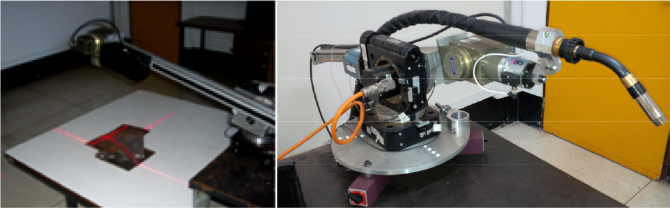
Robot prototype
3. Kinematic System
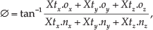
3.1. Assignment of joint coordinate frames
For the construction of the forward kinematic model, joint coordinate systems were assigned in such a way that the
The origin of the base frame coincides with the origin of the first joint, whose axis is perpendicular to the x-y plane. The origins of the other joint frames are placed as follows: (a) if the joint axes of a link intersect, then the origin of the frame fixed to the link is placed at the intersection of the joint axes; (b) if the joint axes of a link are parallel or do not intersect, then the origin of the frame fixed to the link is placed at the distal joint. Thus, the coordinate frame i is placed at joint i + 1, i.e., the joint that connects link i to link i+1; (c) if a frame origin is described relative to another coordinate frame including more than one direction, then it must be moved in order to have its relative position described by only one direction, if possible. Thus, the origins of the coordinate frames are described using a minimum number of link parameters [23].
A coordinate frame is attached to the end-effector such that the z-axis of the frame has the same direction as the z-axis of the frame placed at the last joint (n-1). For this robot, it is also necessary to have a separate transformation for this last frame, which is fixed at the welding torch tip, to ensure that its z-axis is parallel to the axis of symmetry of the torch nozzle, ensuring a proper control of the welding torch's orientation.
The nomenclature used to represent link length parameters has an index for joints and direction. The pki length is the distance between the origins of the coordinate frames i-1 and i, and k is the axis of the coordinate frame i-1 that is parallel to the length direction. Figure 2 shows the previous rules applied to the robot constructed with all coordinate frames, geometric parameters and link variables.
3.2. Forward kinematic model
Homogeneous transformation matrices relating coordinate frames from the base (b) to the torch/tool (t) can be derived as follows:
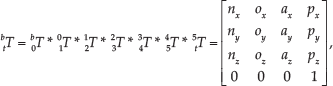
where
The transformations shown in Eq. (1) can be described using the Denavit-Hartemberg (D-H) convention, as below:
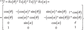
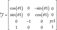
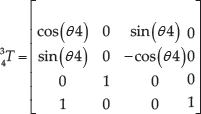
where θ and α are rotation parameters and d and l are translation parameters. The application of Eq. (2) to each of the consecutive robot joint frames by using the geometric parameters shown in Figures 2 and 3 produces the following homogeneous transformations:


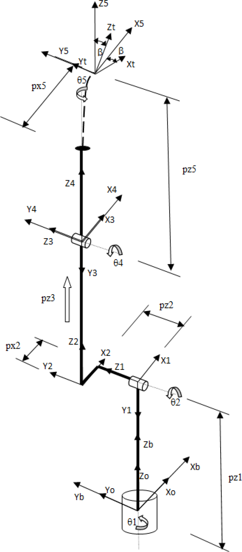
Robot at zero position with joint coordinate systems and link variables

Welding torch coordinate frame (xt, yt, zt) and related geometric parameters (tx, tz)
The next and final homogeneous transformation rotates the Coordinate System 5 around the

The elements of the general manipulator transformation,


3.3. Inverse kinematic model
It is supposed that the vision sensor provides the normal vector to the surface to be welded,
According to the kinematic model in Figure 2, with θ5 at its zero position, the vectors
It is assumed that
The robot position with the torch coordinate system oriented when the angle θ5 = 0

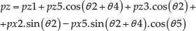
in which
The triplet

The vectors
A general orientation transformation Hp0 can be formulated as:

whose first three columns determine the components of the vectors
The robot's inverse kinematics provide all the joint values in Eqs. (9) to (20). However, Eq. (1) is not equal to Eq. (22), except in the case of θ5 = 0.
Particularly, the equations of the robot's inverse kinematics can be found geometrically. For that purpose, the torch coordinate frame should be rotated by an angle -β around

The transformation
Equations (17) and (18) can be manipulated algebraically to make θ5 explicit. There are two solutions for θ5:

If the component of the product
From Eqs. (11) and (15), and by using the orthonormality of the rotation matrix below:

θ1 can be made explicit as:


The equations above present a singularity for az = ∓ 1, i.e., nz = oz = ax = ay = 0, where the flange
The correct solution for θ1 must be chosen from the sign of the z components of the normal vector to the plane π formed by the vectors
Closed equations for the joint variables θ4, θ2 and pz3 cannot be easily formulated from the robot's general transformation matrix, but they can be expressed using geometry. From Eqs. (23) and (7), one can determine the position of the origin of the coordinate frame 4,

where the origin position is described from the entries of the fourth column of the
From Figures 4a and 4b, pz3 can be obtained as:

in which
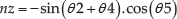
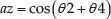
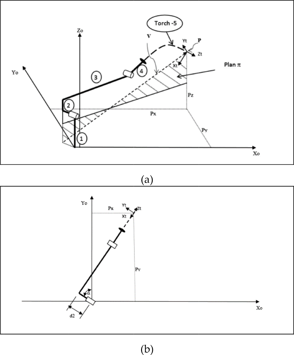
The variable θ2 can be formulated from:
The variable θ4 can be obtained from:

It is clear from the equations above that θ5, θ1 and (θ4+θ2) only carry information from the torch orientation, while pz3, θ2 and θ4 define its position.
4. Algorithm for Searching the Correct Inverse Kinematics Solution
Equations (24), (26), (27), (29), (30) and (31) provide an explicit solution for the inverse kinematics, assuming proper values for the welding-torch orientation vectors,
A solution to this problem is the use of an iterative method that varies
4.1. Algorithm description
Since a welding torch has a cylindrical geometry, one can assume that the rotation around its symmetry axis does not need to be specified (around
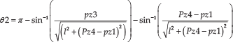
The algorithm principle is based on the calculation of the relative angle, φ, between two 2D rotation matrices. An arbitrary reference angle is the guess for the triplet

The matrices above are orthonormal. Two properties of orthonormal matrices ensure that the scalar product between two columns/rows is null and that the norms of the columns/rows are unitary. Then, it can be easily demonstrated that:


where φ is the relative rotation angle of the pair [X
The torch orientation,
equation (23) is used to rotate the triplet
Equations (24–31) are used to determine the joint variable values,
Equations (9–20) are applied to calculate the forward kinematics, finding the robot position,
The difference between the position specified,
Once the vectors
It is assumed that each value of φk in an iteration corresponds to a

Therefore,


Positioning error of the welding torch in each iteration k
equation (36) provides a new rotation value φk+1, ∀k:(1≤k≤n), in each iteration k, until the error en+1 between
4.2. Results of the inverse kinematics algorithm
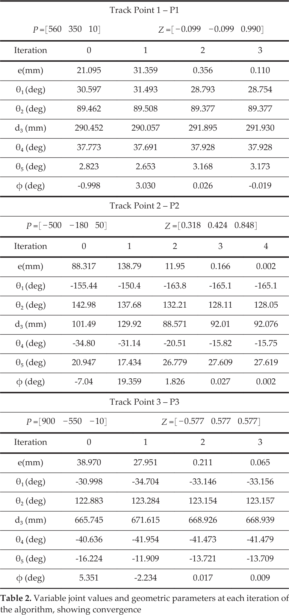
To check the algorithm's efficiency in order to calculate the inverse kinematic iteratively, different robot poses were inputted. All cases have demonstrated that the algorithm converges to the solution with three to four iterations. The input variables are the position of the welding point to be welded and the normal vector to the surface obtained from the vision sensor (
The robot dimensions were determined as shown in Table 1, after calibration, discussed in subsequent sections.
Robot geometric parameters, according to Figure 2, after model calibration


Graphical demonstration of the rotation of
Three cases of position data in three different quadrants of the robot workspace and torch orientation were inputted into the iterative algorithm as shown in Table 2. Results show the convergence of the joint values and the algorithm parameters.
The chosen value for ε was 0.15 mm, but it can of course be higher. This error threshold most of the time interrupts the algorithm typically in the third iteration. Of course, the poses were chosen to be feasibly reached by the torch. Some indetermination could be found when θ1 was close to 45°, 135°, 235° and 315°, but the singularity can be easily avoided with a forward and backward coordinate transformation. The robot was tested at many different positions and orientations during welding and no singularities were found.
Variable joint values and geometric parameters at each iteration of the algorithm, showing convergence
The results of the inverse kinematics were used in the forwards kinematic model to check the accuracy of the algorithm, and the results are shown in Table 3. Physical measurements of the tracking process are not always feasible and were not performed, furthermore the position accuracy depends on that of the kinematic model after calibration. This matter will be discussed in the following sections. Figure 7 shows a weld bead welded by the robot, with a speed of 10mm/s in a straight line. Details of the control system will not be presented in this article.

Weld beads, welded by the robot at a speed of 10mm/s
Position and orientation errors of the inverse kinematics for each of the three track points within three different quadrants

5. The Robot Calibration System
Robot calibration is the process of improving the robot's accuracy by modifying its nominal kinematic model in the robot controller. Robot calibration can be divided into two main groups: static and dynamic calibration [24].
Static calibration systems calibrate geometric parameters, such as joint positions and axis misalignments, and also non-geometric parameters, such as link and joint elasticity, gear errors (eccentricity and transmission errors), gear backlash and thermal expansion. Both geometric and non-geometric parameters can be included in static calibration models because these parameters can be identified only using robot pose data. Although there are some publications [25, 26] related to non-geometric parameter calibration, these extra parameters increase significantly the complexity of the model. It has been reported [27, 28] that the different types of parameters follow an order of quantitative importance for improving the accuracy of kinematic models: geometrical parameters, joint elasticity and link elasticity. Transmission and coupling (i.e., gear parameters) have little influence on increasing the model accuracy. This article will consider only static calibration with geometric parameter errors, since this type of parameter is the main source (≈ 90%) of pose errors in industrial robots [28].
Dynamic robot calibration has importance only in large robots at high speeds and accelerations, requiring extensive and difficult experimental procedures [29, 30], which does not correspond to this case.
In general, a robot calibration system consists of an external measurement system, a calibration model including the parameters to be calibrated and the robot controller, as shown in Figure 8 [31].
In this work, the measurement system used was a Measurement Arm ITG ROMER, with an accuracy reported by the manufacturer of 0.087 mm. The measuring arm was used to measure the positions of the welding torch tip mounted on the robot flange, in several locations within its workspace. The system can be seen in Figure 9.
The procedures for robot calibration have four steps: (a) kinematic modelling, (b) position measurements, (c) parameter identification and (d) kinematic parameter updating or model compensation.

Block diagram of a robot calibration system

ITG ROMER measurement arm
5.1. Parameter identification modelling
Robot calibration consists basically in the problem of fitting a nonlinear model to experimental data. As a result, error parameters are identified by minimization of an error function.
A robot kinematic model is a complex non-linear function that relates link geometric parameters and joint variables to the robot end-effector pose, such as in:

where P is the manipulator transformation, Ti are the link transformations defined in Eq. (1) and n is the number of links. A kinematic model using the D-H convention can be expressed as (from Eq. (2)):

where θ, α, d and l are parameters defining the transformation from a robot joint frame to the next joint frame, where d and l are translation parameters and θ and α are the rotation parameters.
The partial derivatives shown in Eq. (39) represent the contribution of the pose errors produced by each of the geometric error parameters of each joint, producing the total pose deviation of the robot′s end-effector, which can be measured physically. Considering the measured robot pose (M) and the transformation from the robot base frame to the measurement system (B), then ΔP is the vector shown in Figure 10.
The transformation B can also be seen as a link that belongs to the robot model and has to be identified. Then the error value ΔP can be calculated using Eq. (40).

The transformation P can be updated iteratively each time a new set of geometric parameters are identified, and the calibration process ends up with P minimizing the deviations from the measured poses.
Rewriting Eq. (39) in a matrix form for various measured poses of the robot end-effector, Eq. (40) can be rewritten as the Jacobian matrix containing the partial derivatives of P, since Δx is the vector of the model parameter errors as:


Calibration transformations
The size of the Jacobian matrix is a function of the number of measured points measured in the workspace (m) and the number of error parameters in the model (n). The matrix order is (ηm x n), where η is the number of space degrees of freedom (three positions and three orientation parameters). Thus, the calibration problem is reduced to the solution of a non-linear system of the type
There are many methods available to solve this type of system and one that is widely used is the Squared Sum Minimization (SSM). Numerous publications that discuss these methods and related algorithms extensively can be easily found [32]. A widely used method for solution of nonlinear least squares problems, which is successful in practice, is the algorithm proposed by Levenberg-Marquardt (L-M algorithm). Several versions of this algorithm have proved to be globally convergent. The algorithm turns out to be an iterative solution method by introducing few alterations in the Gauss-Newton method to overcome numerical divergence problems.
Each iteration of the algorithm follows three steps, where xk is the parameter vector of the kinematic model in the k th iteration and Δx k are the corrections to be inserted into the model [23], described by the following:
Calculation of the robot's Jacobian (
Calculation of the vector

Update
where μk is obtained from the relations as expressed in Eq. (42).

5.2. Kinematic modelling for robot calibration
In parameterized kinematic models for robot calibration, three properties are the most important: completeness, continuity and minimality [24]. Completeness is regarded as the ability of the model to describe every possible geometrical variation in the links and joints of a robot. Continuity and minimality characterize proportion and redundancies in parameters of the calibration model, respectively.
In our case, the robot has only perpendicular axes. The D-H convention, shown in Eq. (2), can be safely used in parameterized error models when modelling perpendicular axes, which is not true for parallel axes due to singularities that occur in the Jacobian matrix. This topic is discussed in detail in [23].
The transformations shown in Eq. (40) have to include parameterized errors in the kinematic model for the robot calibration. The geometric parameters included in the identification model of this robot can be seen in Table 4, where δs are the error parameters that model the geometric differences between the robot nominal model and the corrected model, which is closer to the actual robot. The parameters can be identified by the calibration system algorithm and are all initialized to zero. The transformations between the world coordinate frame (at the frame origin of the measurement system) and the robot base coordinate frame (W–B), joint to joint transformations (
The first (W-B) and the last (JR - JTCP) transformations shown in Table 4 are the transformations that locate the coordinate system of the robot base with respect to the world coordinate system, and the TCP with respect to robot flange, respectively. As both systems can vary in position and orientation that cannot be measured, it is necessary that their elementary transformations belong to the Euclidean group, with six parameters. However, if only position data are measured in the TCP with the external measurement system, there is no need to include orientation error parameters in the last transformation.
Initial robot kinematic model parameters and transformation equations. (⊥ = perpendicular, R = rotary, P = prismatic, W = world, B = base)

A proper choice of the error parameters to be included in the identification model is very important to ensure the minimality and continuity of the model, such that the error parameters do not impose parametric redundancies that produce ill-conditioned solutions into the nonlinear identification routines. Therefore, a finite number of parameters may have to be excluded from the complete model shown in Table 4. The mathematical basis and the strategies to optimize the model parameterization and ensure a good model fitting are discussed in the next section.
6. Kinematic Model Optimization
A very useful tool to analyse, evaluate and optimize kinematic models and parameter identification routines is the Singular Value Decomposition (SVD) [32] of the J matrix, which is an algorithm equivalent to a linearization in the least-square sense. The SVD is a powerful tool to deal with equations or matrices that are either singular or numerically quasi-singular.
The Jacobian matrix in Eq. (41) can be written as (h = 3.m if only positions are measured):

where the number of rows, h, is larger than or equal to the number of columns, n; S is a square diagonal matrix with positive or null entries; U is an orthogonal matrix and VT is the transpose of an orthogonal matrix. This matrix decomposition is always possible, no matter how ill-conditioned the J matrix is.
If J has rank r, the singular values of S can be ordered to be non-increasing such that all values are non-negative and exactly r of them are positive.
6.1. Condition number
In numerical analysis, the condition number can be viewed as an observability index [33] of model parameters to be identified. It can also be considered as an amplification factor in numerical perturbation and error analysis [32].
The condition number of the matrix J can be calculated from:

where
If the previous norm is Euclidean, the condition number can be directly calculated from the largest, S 1 , and the smallest, S r , non-zero singular values as:

6.2. Jacobian column scaling
A procedure to improve the Jacobian matrix condition can be implemented by performing column scaling. Scaling factors can be valuated from the expected error of the robot (≅ 1 mm) [24, 34]. These factors can be calculated using the model function P(x) (Eq. 38), by using the first-order approximation in xk:

where x=[x1T, x2T,…, xnT]T, n is the number of parameters and q is the robot pose.
For the robot pose q, the value

is the parameter variation that, using a first-order approximation, produces a TCP's position displacement of 1 mm. The denominator is the norm of the kth column of the Jacobian.
If the σxk(q) values are calculated for a large set of joint positions, q=[q1,…, qm], without restriction of position and orientation, the values

are very close to the minimum deviation among all possible positions [24]. The σxk values are denominated as extreme values and are to be employed for column scaling of the linearized least-square system in Eq. (41).
6.3. Optimization scheme
The main purpose of calibration model optimization is to reduce the number of parameters in the model in order to eliminate dependencies or quasi-dependencies between them, not to the point of restricting the model accuracy but far enough so that the condition number of the scaled Jacobian is less than 100. The experience of research groups in mathematics demonstrates that a condition number smaller than 100 is required for reliable results [24, 32].
Therefore, the procedures for model optimization can follow the following steps:
Model-based scaling (Eq. 48) using extreme scaling values must be computed to reduce the condition number k(J) many times.
Quasi-dependencies and non-identifiabilities are pinpointed by investigating the column vector V r corresponding to the smallest singular value S r of the SVD as follows:

and so

If J has rank r, then S r+1 =… = S n = 0. The optimization procedure is then performed by following the two previous steps. The first step improves the condition k(J). If k(J) is higher than 100 then the next step determines the model parameters that produce rank deficiencies. Thus, an optimal model is obtained by excluding a small number of parameters from the complete model successively, until K(J) is less than 100 during the parameter identification routine. However, in practice, most of the available pose measurement systems used in robot metrology (ultrasound, contact, CCD cameras, laser systems, theodolites, etc.) have an accuracy ranging from 0.05 mm to 0.5 mm, depending on its type and complexity. If measurement noise is increased by using measuring systems with lower accuracies, then usually k(J) is also increased, and the threshold of k(J) = 100 will not be achieved by excluding only a few parameters from the model. If that is the case, the routine of the kinematic model optimization stops if k(J) has only a small reduction on the exclusion of one more parameter. It is important to note that the optimization procedure described aims to exclude the most redundant parameter from the parameterized model at a time. In this way, regardless of the number of parameters in the model, there will always be an improvement in the condition number with the exclusion of another parameter. However, if a parameter is removed from the parameterized model that has not been identified by the optimization routine then there will be no guarantee that the condition number will improve, or that there will be an improvement in the kinematic model accuracy.
7. Experimental Results
The model optimization method aiming at eliminating redundant parameters from the calibration model was tested in an experimental procedure, where the actual robot had been measured at 24 positions that were selected to cover a large range of the robot's joint positions. The results of the experiment are shown in Table 5.
Statistics of the calibration process as a function of the number of parameters to be identified in the model

The calibration process was initially carried out with the maximum number of parameters shown in Table 5. The algorithm stopped when the Euclidean norm of the parameter error vector did not change significantly. Equations (49) and (50) were then used to calculate the condition number, K(J), and to identify the parameters corresponding to the smallest singular value in a model, easily observed from the largest entry in the last column of the scaled V matrix. Frequently, two parameters have approximately the same largest value in the interval 0<vi<1, where vi is the entry in the ith line of the last column of V, which means that they are mutually redundant. The parameter to be eliminated from the model is the one with a null value in the nominal model (not necessary for the nominal model).
The results showed in Table 5 show clearly that as long as a parameter is removed from the model, the condition number of the Jacobian reduces as well. The model with 18 parameters presented a condition number below 100 in the sequence. That coincides with the smallest average position error.
However, the precision of the calibrated model has to be checked moving the robot to other points than the ones at which the measured points were collected. Therefore, the accuracy evaluation step is to correct the nominal model using the parameter errors obtained from the calibration routine and to proceed the measurement process at other locations, but calibrating only the first six parameters of the model, i.e., only the robot base parameters.
The robot was evaluated at another quadrant of the workspace, far from the region at which it had been previously calibrated. The results shown in Table 6 demonstrate that the highest accuracy had been obtained using the model with 18 parameters. One can realize that the robot's position accuracy had improved each time that a parameter had been removed, and started decreasing when the number of parameters was below 18. This behaviour clearly agrees with the mathematical concepts of completeness and minimality, which means that too many parameters produce redundancies in the kinematic model and using fewer parameters than is necessary cannot model the robot's geometry completely.
Statistics of the calibration evaluation procedure, with robot joint positions other than the ones used to calibrate the model, within another quadrant of the workspace.

The parameter optimization scheme had been proved to be successful, pinpointing the optimal error parameter vector to be identified in order to improve the robot's accuracy.
8. Conclusions
This article presented a robot constructed to repair hydraulic turbine defects by welding in layers automatically by using a 3D surface map acquired from a specialized vision sensor. The discussion focused on the kinematic model, the algorithm to perform the iterative inverse kinematics and the mathematical procedure for parameter-identification optimization of the robot's calibration system.
Experimental results showed that the iterative algorithm for inverse kinematics is very efficient, converging to the solution in three to four iterations and showing very good tracking. Experimental work with welding in straight lines also proved the reliability of the solution. The mathematical scheme to find the optimal set of geometric parameters for robot calibration proved to be efficient and simple, able to find the best set of geometrical parameters to be identified by the robot's calibration procedures, leading to the best accuracy for the robot model among all possible parameter sets.
Footnotes
9. Acknowledgements
This work had been supported by ELETRONORTE (Electrical Power Plants of the North of Brazil) and FINATEC (Foundation for Scientific and Technological Enterprises).