Sage Journals: Discover world-class research

Abstract

This paper proposes a joint-space trajectory generation method for practical navigation with a high curvature path of mobile robots. A technique to generate central velocity commands using a convolution operator that considers only the physical limits of a mobile robot was discussed. In practical application, controlling the heading angles along a curved path is required and the existence of obstacles is inevitable. First, we suggested an algorithm that generates a trajectory to consider the heading angles along a smooth Bezier curve by redefinition of the curve parameter. However, the presence of an obstacle along the planned path requires redirection to a new path where geometrical limitations such as high curvature turning points exist, resulting in tracking error. We propose a method that manages a variation of linear interpolation to generate a feasible trajectory while conserving the high curvature path and the merits of convolution. Joint-space trajectories are produced by scaling down the generated central velocity through reduction of the given maximum velocity limit. We show through a simulation example that the proposed method is able to generate a trajectory that can accurately track a planned path on a designed platform based on actual parameters. Finally, an experiment is successfully conducted on a two-wheeled mobile robot, Tetra DS-III, in a real-time control system. The experiment results display distinct advantages in the criteria of time optimality and periodicity of control tasks, while conserving all possible limitations that could occur during navigation compared with previous studies.

Keywords

Two-Wheeled Mobile Robots Joint-space Trajectory High Curvature Path Convolution Bezier Curve

1. Introduction

Ceaseless studies and the development of mobile robot systems have made it easier for users to manipulate robots in order to show precise motion control through the generation of uncomplicated velocity commands. This has widened the range of applications in the fields of manufacturing and security and studies in the commercial and industrial sectors. Currently, mobile robot application domains have extended into residential areas in the form of domestic, educational, or entertainment autonomous robots. Another outstanding result of this development is that places beyond the reach of humankind are now accessible through the appropriate operation of these robot systems, such as space missions, hazardous environments and military operations [1 –3].

In a known environment, mobile robot navigation is a systematic operation composed of three main phases: path planning [4–5], trajectory generation [6–7] and tracking control [8]. Path planning considers the generation of a predetermined path for the mobile robot to follow from an initial point to a desired terminal point in a working environment. Various types of geometric curves are usually employed in path planning, such as precise single-curvature curves [9], cubic splines [10], cubic spirals [11–12] and Bezier curves [13 –15].

Trajectory generation produces the required velocity commands for the robot to transverse the planned path as a function of time. In other words, a trajectory generator produces predefined velocities for the robot to track a planned path. To obtain feasible trajectories, various physical and dynamic constraints are considered during trajectory planning. The movement of mobile robots can be constrained or not, depending on their physical limitations such as maximum velocity and maximum acceleration. Further accuracy and rigorous control along a planned path based on a higher polynomial curve requires consideration of the third positional derivative, maximum jerk limit. These physical limitations are highly conserved in order to avoid potential damage and produce remarkable results in terms of position tracking.

Lee et al. [16] suggested the use of a convolution operator to generate a trajectory using the physical system limitations of the mobile robot. The advantages of this method are classified into three main parts: continuous differentiable trajectory obtained using convolution, a resulting trajectory that always satisfies the given physical limitations and a low calculation burden due to the recursive form of convolution. However, the generated trajectory only considers the linear distance between the initial and terminal points and not the heading angles at each point of a given planned path based on a Bezier curve. In our previous work [15], we presented a solution to this problem by formulating the defining parameter of a Bezier curve as a function of the total travelling time.

Although these methods show appealing results on a smooth curve, it is more likely for a mobile robot to encounter obstacles in many service applications where it needs to share its work region. Common obstacle avoidance techniques [17 –22] involve redirection of the mobile robot to a new path where geometric constraints, such as high curvature turning points, occur. These constraints greatly affect robot control, producing issues of accuracy, such as the inability to track the planned path, non-uniform time sampling, or undesirable terminal velocities [14]. Thus, a trajectory planning method that also considers the geometric constraints is required.

In this paper, we address the high curvature problem using an algorithm based on a variation of linear interpolation to conserve the desired trajectory instead of smoothing the planned path. First, a smooth curve based on a Bezier curve is produced as the planned path for the mobile robot to track. Accordingly, velocity commands are generated using the trajectory generation method based on convolution in our previous work to satisfy the physical limits of the mobile robot and the heading angle along the planned path. Assuming that an obstacle is present in the working environment, the mobile robot is redirected to a new path, which is governed by geometric constraints. The proposed method calculates the displacement at each sampling point along the path and reformulates the velocity commands using linear interpolation to maintain periodicity and generate a practical trajectory. However, actuation of the mobile robot requires velocities in the joint-space that can provide different results, even when the central velocity satisfies the velocity limit. To consider the joint-space velocity limitations, a downscaling scheme presented in another previous work [23], which adjusts the configured maximum velocity limit, was also conducted. Finally, we applied our method to a two-wheeled mobile robot, Tetra DS-III. For practical applications, we developed cyclic tasks in real-time operating systems, such as Xenomai [24]. Robot controls that use real-time operating systems require the velocity commands in uniform sampling time, meaning that the velocity commands of two wheels should be generated in uniform sampling time in order for the robot to be actuated within.

This paper is organized as follows: Section 2 presents a review of the convolution-based trajectory generation. Section 3 discusses a path planning technique based on a Bezier curve. Section 4 examines the central velocity generation based on convolution, which considers the heading angles of a smooth Bezier curve and the proposed trajectory generation technique that solves the geometrical problem encountered during obstacle avoidance. Simulation and experiment examples are presented in Section 5 to confirm the validity of the suggested method in the described working environment. The final section draws the conclusion.

2. Convolution-based Trajectory Generation

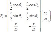
As shown in Figure 1, the actual position of the mobile robot is shown in both real and robot world frame coordinate systems. To describe the location of the mobile robot numerically, the central position in the global Cartesian coordinate system, P_c, is determined as:

Figure 1.

Kinematic model of a two-wheeled mobile robot

P_{c} = [\begin{matrix} x_{c} & y_{c} & θ_{c} \end{matrix}]'

(1)

where (x_c, y_c) denotes the coordinates and θ_c denotes the heading angle obtained in the anticlockwise direction from the x-axis.

From this notation, the central velocity profile is generated through various approaches, such as consideration of the acceleration limitations of the mobile robot with respect to the curvature of the planned path [10, 14], or through utilization of a convolution operator [15–16].

Lee et al. [16] stated that the convolution operator can generate a central velocity profile that produces a smooth trajectory for a mobile robot while satisfying physical limitations such as maximum velocity, acceleration and jerk. In order to generate the central velocity using a convolution operator, all related physical constraints configured within the mobile robot are required. The following equation defines a square wave function, y₀(t), with an area equal to the total distance of the planned path, S:

\begin{array}{l} y_{0} (t) = {\begin{matrix} v_{0}, 0 \leq t \leq t_{0} \\ 0, o t h e r w i s e \end{matrix} \\ where, t_{0} = \frac{| S |}{v_{0}} \end{array}

(2)

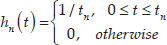
A square wave function with unit area defines the nth convolution function h_n(t) in the section 0 ≤ t ≤ t_n, which is expressed as follows:

h_{n} (t) = {\begin{matrix} 1 / t_{n}, 0 \leq t \leq t_{n} \\ 0, o t h e r w i s e \end{matrix}

(3)

where t_n depends on the given physical limitations that represent the overall time duration, that is:

t_{n} = \frac{v_{m a x}^{(n - 1)}}{v_{m a x}^{(n)}} f o r n = 0, 1, 2, \dots i

(4)

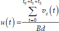
The function y_n(t) is the result of the nth time convolution operation between the unit function h_n(t) and a velocity function with the maximum value $v_{0} = v_{max}^{(0)}$ . $v_{max}^{(1)}$ is the first-order velocity function with the maximum value $a_{max}$ , which is the maximum acceleration limit. $v_{max}^{(2)}$ is the second-order velocity function with the maximum value $j_{max}$ , which is the maximum jerk limit.

By applying the preceding output of the system as input, the successive operation of digital convolution in uniform sampling time T_s generates a trajectory described by the simplified recursive equation:

\begin{array}{l} v_{n} (t) = y_{n} [k] = \frac{y_{n - 1} [k] - y_{n - 1} [k - m_{n}]}{m_{n}} + y_{n} [k - 1] \\ k = t / T_{s}, m_{n} = t_{n} / T_{s} \end{array}

(5)

This method produces a differentiable central velocity profile that generates a trajectory that considers the physical limitations of the mobile robot for a given linear distance.

3. Path Planning Based on a Bezier Curve

Path planning is finding a path from a starting position to a desired position in a workspace. The path of a robot can be viewed as a series of mathematical operations that involve translation and rotation from the initial to the terminal point. Various approaches are used in path planning and one of the most commonly used curves is the Bezier curve.

A Bezier curve is a parametric curve named after its originator, Pierre Bezier, who used the mathematical method for drawing models in manufacturing automobile bodies for the French car company Renault. Bezier curves use Bernstein polynomials as a basis and they differ from other types of curves in that they consider the heading angles from both the initial and terminal points. Moreover, the curve does not have to pass all the control points that define it. Instead, a polygon is drawn by combining all control points and the curve is located within this polygon. In other words, the drawn curve always lies on the convex hull of the control points, which solves a computational geometry problem. These advantages increased the popularity of Bezier curves for mobile robot path planning and trajectory generation. A cubic Bezier curve is formulated through an initial point P, terminal point S and control points Q and R. The parametric equation of a cubic Bezier curve is expressed as:

\begin{array}{l} x (u) = A_{0} {(1 - u)}^{3} + 3 A_{1} u {(1 - u)}^{2} + 3 A_{2} u^{2} (1 - u) + A_{3} u^{3} \\ y (u) = B_{0} {(1 - u)}^{3} + 3 B_{1} u {(1 - u)}^{2} + 3 B_{2} u^{2} (1 - u) + B_{3} u^{3} \end{array}

(6)

where u is an arbitrary value within 0 ≤ u ≤ 1 for the parameter that defines a precise smooth Bezier curve, as shown in Figure 2.

Figure 2.

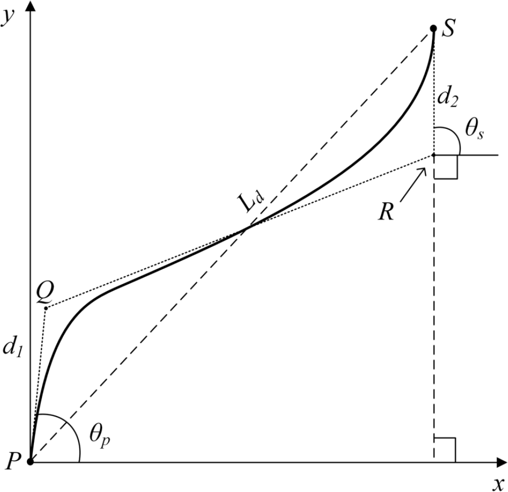
Planned path based on a Bezier curve

In this figure, the estimated initial and terminal points of the robot are at the first and fourth control points, respectively. The second control point, Q, is calculated using the heading angle at the initial position θ_p and the length of the polygon side d₁. In perspective, the third control point, R, requires the terminal heading angle θ_s and length d₂. To avoid misconception, L_d represents the linear distance between the initial and terminal points, P and S, which is not the actual travel distance along the entire path.

4. Convolution-based Trajectory along a Bezier Curve

4.1. Smooth trajectory generation

As a conventional convolution-based trajectory only considers the linear distance between the initial and terminal points, our previous work [15] presented a trajectory generation technique to produce a central velocity generation method for a mobile robot to track a planned path based on a Bezier curve.

Assume that a path based on a Bezier curve that considers the heading angles at each sampling point from an initial position P to a terminal point S is generated by uniformly accumulating a parameter with constant value u and that it is represented as Δρ(u). Then, the total travel distance along the curved path, B_d, is calculated as follows:

B_{d} = \sum_{u = 0}^{1} Δ ρ (u) = \sum_{u = 0}^{1} \sqrt{{(x (u + Δ u) - x (u))}^{2} + {(y (u + Δ u) - y (u))}^{2}}

(7)

In this equation, the smoothness of the curve is defined as inversely proportional to the value of the defining parameter. In other words, as the value of u parameter becomes smaller, a smoother curve is generated. The area of the input function for the convolution operator in the previous section is equal to the travel distance of trajectory S, as shown in Figure 3. To synthesize the convolution-based method in generating a trajectory for a curved path, input S is made equal to the actual distance computed in (7). Hence, velocity v_c(t) is generated assuming that S = B_d, which possesses the properties of convolution, considers the physical limitations of the mobile robot in generating a smooth path. Here, physical limitations, such as maximum velocity, acceleration, jerk and sampling time are set arbitrarily according to the specifications of the mobile robot. Total time duration and required sampling time depend on these physical limitations, as expressed in (4).

Figure 3.

Convolution-based trajectory

However, the generated central velocity v_c(t) for distance S does not yet consider the heading angles along the Bezier curve. In order to consider the heading angles at any position in the task space, which depend on velocities in paths with heading angles, the reformulated defining parameter of a Bezier curve, u(t), is calculated using (8) in the time domain. The accumulated distance at each sampling point in the time domain Δρ(u(t)) is obtained by substituting the calculated u(t) parameter in the Bezier polynomial equation in (6) to produce a trajectory that considers the heading angles of the Bezier curve. In this notation, the shorter the sampling time, the more accurate the generated trajectory in tracking the predetermined path will be.

u (t) = \frac{\sum_{t = 0}^{t_{0} + t_{1} + t_{2}} v_{c} (t)}{B d}

(8)

where u(t) is defined as 0 ≤ u(t) ≤ 1, which serves as the reformulated parameter of the Bezier curve trajectory, depending on the central velocity generated through a convolution operator.

This transformation generates a trajectory that will incorporate the characteristics of the convolution operator in satisfying the physical limits of the robot in uniform sampling time while also considering the heading angles along the Bezier curve-based path.

4.2. Obstacle avoidance

In a practical application, mobile robots typically share their working environment with a variety of obstacles. Jolly et al. [14] proposed an obstacle avoidance approach through the generation of consecutive Bezier curves. In the presence of an obstacle, a redirection is made from a certain point by generating two additional Bezier curves from the original path, as shown in Figure 4. A collision between robots occurs when the centre of a robot crosses the calculated safety margin.

Figure 4.

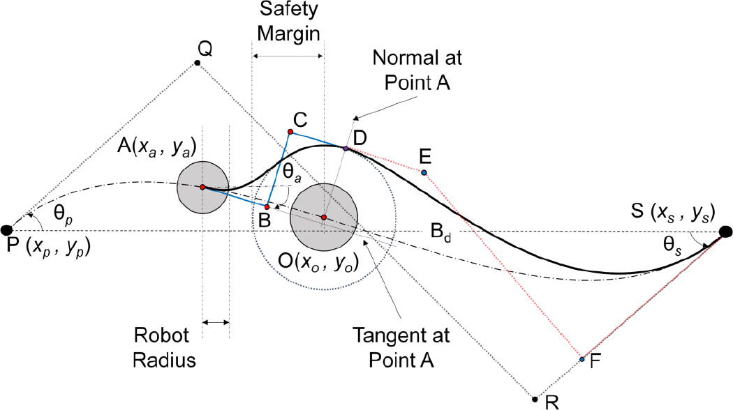
Obstacle avoidance algorithm

The original planned path is defined by the control points PQRS. The robot changes direction to avoid colliding with the obstacle located at point O by generating two consecutive paths. The first section of the redirected path is from point A, where a new path is generated using a Bezier curve described by polygon ABCD. Depending on the location of the obstacle and the position of point A, the first section of the redirected path can contemplate high curvature values at its turning points that impose problems in controlling the mobile robot. Another Bezier curve is generated from the end point of the first section for the mobile robot to return to its original track and reach the targeted terminal point. The second section of the path is defined by polygon DEFS.

Lepetič et al. [10] proposed a velocity profile generation technique that considers the acceleration limitations of the mobile robot and its relationship with the curvature of the path. The maximum possible velocity of the robot at each sampling point is restricted by the curvature, κ, defined in (9) as:

κ (u) = \frac{\overset{\cdot}{x} (u) \overset{\cdot\cdot}{y} (u) - \overset{\cdot}{y} (u) \overset{\cdot\cdot}{x} (u)}{{(\overset{\cdot}{x} {(u)}^{2} + \overset{\cdot}{y} {(u)}^{2})}^{3 / 2}}

(9)

If the radial acceleration of a point is lower than the maximum radial acceleration limit, the corresponding velocity can be realized. To satisfy the radial acceleration of the mobile robot, the velocity is calculated from the initial, terminal and turning points. Turning points are those points along the curve that show the highest local curvature values. The minimum value at each point of the combined velocity profiles is considered to be the maximum allowable velocity to actuate a mobile robot.

Although this approach considers the high curvature turning points of the path, other physical limitations of the mobile robot, such as maximum velocity and jerk limitations, are not considered. The generated velocity is calculated in the parameter u-domain and the actual travel time of actuation is computed by integrating the calculated time differences at each sampling point. In case of zero velocities at either the initial or terminal points, inaccurate time differences occur according to the distance formula, which leads to infinite values and unpredictable results. Another issue not to be neglected is periodicity. Non-periodic velocity commands are considered difficult to realize in practical applications, for example, cyclic tasks in real-time operating systems, such as Xenomai [24]. Real-time systems require task responses to be kept in strict sampling time or constants. Therefore, robot controls that use real-time operating systems require the velocity commands in uniform sampling time to produce flawless results. In other words, in rigorous robot control, velocity commands should be generated in uniform sampling time in order for the robot to be actuated within.

Moreover, discontinuities between velocities at junctions formed during redirection are present in this procedure. In addition, a configured velocity limit for the mobile robot is also not considered during this path planning method, which is another constraint when contemplating practical mobile robot navigation.

4.3. High curvature trajectory generation

Due to the problems imposed by an established work as explained in the last section, the smooth trajectory generation technique of our previous work is incorporated for obstacle avoidance in order to manage the preceding issues. However, the velocity commands were not able to generate a trajectory that can track the planned path, due to the governing geometric constraints at the high curvature turning points.

A new trajectory planning method that uses the same convolution operator is presented to manage the tracking issue that occurs because of the geometrical constraints along a Bezier curve with high curvature turning points during obstacle avoidance. The central velocity is calculated to correspond with the configuration of the path in order to manage this occurrence.

In smooth trajectory generation, a path is assumed to be generated by constantly accumulating parameter u and transforming it to the time domain parameter u(t). For a path with high curvature, velocity constraints at the turning points require consideration of the infinitesimal displacement of the robot between each sampling point along the curve dS(u(t)), expressed as:

d S (u (t)) = \sqrt{\overset{\cdot}{x} {(u (t))}^{2} + \overset{\cdot}{y} {(u (t))}^{2}}

(10)

where and denote the displacement for each sampling point on the x and y axes, respectively.

Since the displacement at each sampling point is non-uniform, it is certain that the time for the mobile robot to reach each sampling point is also non-periodic.

d t = \frac{d S (u (t))}{v_{c} (u (t))}

(11)

where dt denotes the sampling time for the robot between each point of the curved path and v_c(u(t)) is the central velocity generated through convolution.

To produce the proposed central velocity, a variation of linear interpolation is conducted to reformulate the convolution-based velocity to establish periodicity in reaching each sampling point.

v_{u n i} (t) = v_{c} (t_{n - 1}) + \frac{v_{c} (t_{n}) - v_{c} (t_{n - 1})}{t_{n} - t_{n - 1}} (t - t_{n - 1})

(12)

Here, v_uni(t) is the proposed central velocity; the total time is calculated by integrating the result from (10) and is denoted by t_n; and the uniform sampling time t is defined as t_n-1 ≤ t ≤ t_n. This notation makes the convolution-based velocity comply with the path generated with high curvature in periodic sampling time.

This method is an improvement on our previous research, which generates a central velocity to produce a trajectory that preserves the merits of the convolution operator to satisfy the physical limitations of the mobile robot while considering the geometrical constraints present along the high curvature-planned path.

The sequence of major computations for generating the proposed convolution-based practical trajectory that can track a planned path with high curvature turning points along a Bezier curve is as follows:

Define a planned path through given terminal points and control points in uniform sampling points using (6).

Calculate the total travel distance along path B_d using (7).

Calculate the total travel time for a travel distance B_d, according to the given physical limitations of the mobile robot using (4) with the given maximum velocity, acceleration and jerk values.

With the calculated travel distance and total travel time as inputs, perform the recursive form of the convolution operator in (5) for two successions to consider the physical limits of the mobile robot, such as maximum velocity, acceleration and jerk.

From the curve parameter u-domain, transform the path in the time domain using (8).

To consider the heading angles of the Bezier curve, substitute the transformed parameter in (6) to generate a smooth trajectory.

For a path with high curvature, calculate the displacement at each point of the reformulated Bezier curve using (10). Respectively, calculate the corresponding time to travel to each sampling point using (11).

To generate the proposed method, which considers the geometrical constraints of the path, produce the central velocity in periodic sampling time using a variation of linear interpolation in (12).

4.4. Joint-space velocities

In a previous study [23], it was found that actual velocity commands to actuate a mobile robot require angular velocity for both wheels. Although the central velocity generated in the previous sections satisfied the maximum velocity limit configured within the mobile robot, actual joint velocity commands could exceed the maximum. Therefore, joint-space velocities are constrained within the velocity limit for both wheels of the mobile robot. From (3), the kinematic model of a mobile robot is as follows:

P_{c} = [\begin{matrix} \frac{r}{2} cos θ_{c} & \frac{r}{2} cos θ_{c} \\ \frac{r}{2} sin θ_{c} & \frac{r}{2} sin θ_{c} \\ \frac{r}{D} & - \frac{r}{D} \end{matrix}] ({\begin{matrix} ω_{r} \\ ω \end{matrix}}_{l})

(13)

where r represents the radius of both the robot's wheels, D denotes the distance between the wheels and ω_r denotes the right wheel's angular velocity, while ω_l denotes that of the left wheel.

The angular velocity and radii of the mobile robot's wheels are the parameters to calculate the actuation velocity commands for each of the wheels of a mobile robot. The following equation expresses the joint velocities:

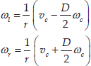
\begin{array}{l} ω_{l} = \frac{1}{r} (v_{c} - \frac{D}{2} ω_{c}) \\ ω_{r} = \frac{1}{r} (v_{c} + \frac{D}{2} ω_{c}) \end{array}

(14)

where v_c represents the central velocity of the mobile robot, ω_c is its corresponding angular velocity, D is the distance between the centre of the two wheels and ω_l and ω_r denote the left and right wheels' angular velocities, respectively. In addition, the following equations define the left and right wheel linear velocities:

\begin{array}{l} v_{l} = r ω_{l} \\ v_{r} = r ω_{r} \end{array}

(15)

ω_c denotes the central angular velocity:

ω_{c} = \frac{d θ_{c}}{d t}

(16)

where θ_c represents the rotational angle at each point of the Bezier curve.

The velocities of the left and right wheels are generated using (14 –16). However, these joint velocities cannot satisfy the maximum velocity limit, although the central velocity can stay within its range. If any of the velocity profiles exceed the maximum velocity limit, the mobile robot displays an inability to track the reference path.

In order to maintain the joint-space velocities within the threshold of the maximum velocity limit, a downscaling scheme that reduces the original maximum velocity limit by a downscaling factor denoted by v_cmax is conducted [21]:

v_{c m a x} = \frac{| m a x (v_{r} - v_{l}) |}{2}

(17)

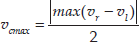
and the downscaled maximum velocity, v’_max, is calculated by:

v'_{m a x} = v_{m a x} - v_{c m a x}

(18)

After calculating the downscaled maximum velocity, the entire process is repeated from the start using v’_max as the newly configured velocity limit.

5. Examples

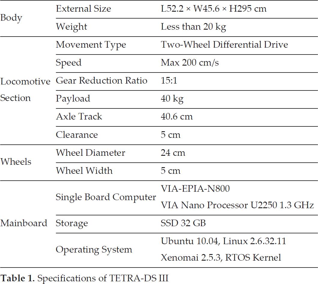
The experimental two-wheeled mobile robot is a TETRA-DS III™ manufactured by Dongbu Robot. TETRA-DS III™ is a high-performance two-wheeled mobile robot platform used to develop autonomous robot navigation technology in an indoor environment. The wheels are powered separately by two AC servomotors and are 24 cm in diameter. The mobile robot is cylindrical in shape and its overall size is limited to 52.2 cm × 45.6 cm × 29.5 cm, without exceeding a weight of 20 kg and payload of 40 kg. To avoid potential damage, configured physical limitations of the mobile robot are considered during path planning and trajectory generation. According to the specifications of the mobile robot, the maximum velocity is 200 cm/s and the maximum acceleration is 200 cm/s².

The detailed physical specifications of the two-wheeled mobile robot are listed in Table 1. During path planning, the maximum velocity limit is readjusted to 120 cm/s in order for the robot to navigate in the prepared experimental environment. The simulations and experiments covered within this study are bound by these values in order to validate the proposed method. Moving a robot within a given working environment requires acquisition of data within its surroundings through mapping. A laser rangefinder is used in order to detect obstacles along the planned path.

Table 1.

Specifications of TETRA-DS III

Body	External Size	L52.2 × W45.6 × H295 cm
Body	Weight	Less than 20 kg
Locomotive Section	Movement Type	Two-Wheel Differential Drive
	Speed	Max 200 cm/s
	Gear Reduction Ratio	15:1
	Payload	40 kg
	Axle Track	40.6 cm
	Clearance	5 cm
Wheels	Wheel Diameter	24 cm
Wheels	Wheel Width	5 cm
Mainboard	Single Board Computer	VIA-EPIA-N800VIA Nano Processor U2250 1.3 GHz
	Storage	SSD 32 GB
	Operating System	Ubuntu 10.04, Linux 2.6.32.11Xenomai 2.5.3, RTOS Kernel

An image of the mobile robot is shown in Figure 5. In this figure, the laser rangefinder is installed at the top of the mobile robot to acquire the data of the working environment with accuracy. The single board computer processes the motion algorithm to be applied and provides the velocity commands and other instructions for the mobile robot, whereas the embedded control board receives all the instructions and controls the movement.

Figure 5.

TETRA-DS III

5.1. Simulation example

In this example, we present a scenario where an obstacle is present along the original planned path. The obstacle causes the robot to transverse into a different route, where the first part of redirection poses high curvature turning points.

The original planned path is designed using (6) with an initial point of (0 cm, 0 cm) with heading angle 0° and initial velocity of 0 cm/s. The terminal point is located at (200 cm, 150 cm) with the same heading angle and terminal velocity of 0° and 0 cm/s, respectively. The obstacle is located along the original path at (100 cm, 75.2 cm) and it is surrounded by a safety margin of 10 cm. The redirection is calculated to start at (34.88 cm, 9.12 cm). The entire synthesis of the planned path to avoid an obstacle is shown in Figure 6. The total travel distance for the planned path is calculated using (7) with the result of 291.17 cm.

Figure 6.

Planned path for a mobile robot avoiding an obstacle

Figure 7 shows the velocity profiles generated considering the acceleration limitations of the mobile robot by researchers [10, 14]. The radial acceleration limit was set to 400 cm/s², whereas the tangential acceleration limit was set to 200 cm/s². The minimum velocity at each sampling point corresponded to the maximum allowable velocity for the robot to travel along the planned path. As shown in the figure, a discontinuity of velocities at the junctions was present and the maximum velocity of 120 cm/s was not satisfied. As the initial and terminal points configured for this simulation are both zero values, calculation of the total travel time for the mobile robot along the planned path is inaccurate given the infinite values at the first and final sampling points.

Figure 7.

Velocity profile considering acceleration limits

Using the same initial values, convolution-based trajectory planning for a smooth Bezier curve was conducted for the planned path. The sampling time was configured to 20 ms. Figure 8 shows the central velocity profile generated using the recursive form of convolution in (5) and its incorporation with a Bezier curve using (8).

Figure 8.

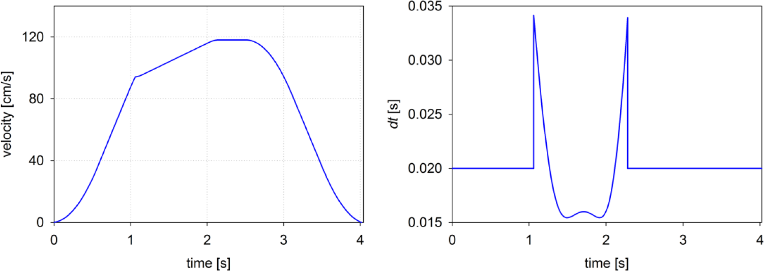
Velocity profile considering the heading angles along a Bezier curve and sampling time difference

Although the convolution-based velocity portrays continuity at the intersection of each redirected path, the actual generated trajectory portrays the inability to follow the given path in a uniform sampling time. The figure also shows the non-periodicity of the sampling time. The total travel distance calculated for this method is 4.02 s, which is faster than the previous method while considering the physical limitations of the mobile robot, but not the geometrical constraints at the high curvature turning points of the redirected path.

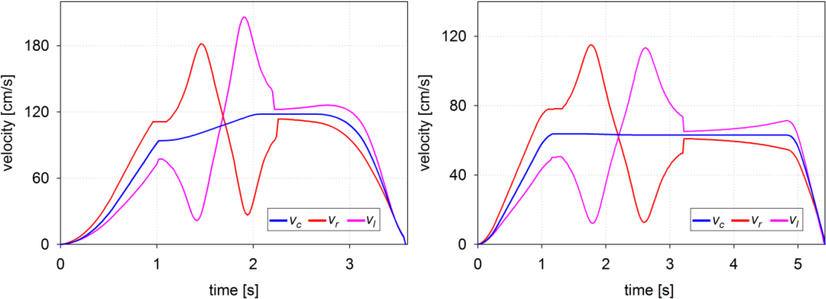
In order to consider the high curvature turning points, the displacement at each sampling point is calculated using (10) and the travel time between these sampling points is calculated using (11). Figure 9 shows a comparison of our previous work, which only considers heading angles along a smooth curve, with the proposed high curvature method by administering a variation of linear interpolation in (12). The total travel time using the method is calculated to be 3.60 s, which is relatively faster than any of the previous methods. The proposed high curvature method was able to track the planned path in the shortest time compared with the other approaches while demonstrating periodicity, being within the physical constraints of the mobile robot, and considering the geometrical constraints of the planned path at the same time.

Figure 9.

Comparison of previous (smooth trajectory) and proposed (high curvature) trajectory generation

For two-wheeled mobile robots, actual velocity commands are given in joint-space. The calculated joint-space velocities of the proposed method are shown in Figure 10. As expected, both the left and right wheel velocities exceeded the configured maximum velocity limit. If the joint-space velocities do not satisfy the velocity limit, it is certain that severe damage and tracking error will occur. To consider the joint-space velocity limitations, the downscaling scheme discussed in section 4.4 should be conducted. The downscaling factor that represents how much the original maximum velocity should be reduced is calculated using (17).

Figure 10.

Joint-space velocities before and after downscaling

In this example, the calculated downscaling factor was 57 cm/s. Thus, using (18), the new velocity limit that allowed the joint-space velocities to be within the threshold of the original velocity limit is calculated to be 63 cm/s. Due to the bounded central velocity, the total travel time for the robot to navigate the same path increased to 5.42 s. The resulting joint-space velocities are also shown in the figure.

The generated joint-space velocity was able to travel along the planned path with accuracy, as shown in Figure 11. The actual velocity commands were given to the mobile robot designed using Marilou Robotics Studio. This simulation was implemented assuming an ideal environment where disturbances such as friction and slip were ignored.

Figure 11.

Simulation results using Marilou Robotics Studio

5.2. Experimental example and results

An experiment was conducted in the working environment illustrated in Figure 12, where an obstacle was placed in the middle of the grid for the mobile robot to detect using the laser rangefinder Hokuyo URG-04LX. The laser rangefinder has the ability to detect objects within 20 mm ~ 4,000 mm in a scan angle of ±120° from its centre. The working environment spans approximately 5.4 m × 5.5 m.

Figure 12.

Actual image of the working environment

There are various approaches to the acquisition of laser rangefinder data [25–26]. Due to the large number of data calculations based on multiple acquisitions of data and the number of data points, the grid sampling method was implemented to map the position data of a certain object. Figure 13 shows the environment map generated from a laser rangefinder where desk areas, divisions and the obstacle are marked appropriately.

Figure 13.

Path planning on the mapped data using LRF

In this case, a simpler example with a static obstacle is considered because of the experiment's setup size limitation. The mobile robot is placed at an initial point of (0 m, 2.5 m) and the target terminal point is at (4.5 m, 3.0 m) with both initial and terminal heading angles set to 0°. The red solid line represents the original path based on a Bezier curve before detection of the obstacle. To avoid a collision with the obstacle located along the original path, the obstacle avoidance algorithm was implemented by generating consecutive redirections defined by the blue dashed line.

Due to the mainboard limitations of the mobile robot, the sampling time between each velocity command was set to 20 ms. The proposed trajectory generation method was compared through implementation on both the generic Linux kernel as the non-real-time operating system and the real-time framework Xenomai, as shown by the comparative illustration in Figure 14. In the case of the real-time system, the mobile robot displayed periodicity and the ability to follow the planned path through the periodic velocity commands, as represented by the black circle in the figure. However, in the non-real-time system, navigation of the mobile robot required a longer time to process each thread of tasks. The delay was calculated to be approximately 0.001657 ms. Due to this delay, the mobile robot was not able to follow the predetermined path, as described by the square box in the figure. From the predetermined initial and terminal points, driving in the real-time system resulted in a more accurate result at each point with the terminal point at (4.478 m, 2.970 m, 0°), whereas the non-real-time system arrived at the terminal point at (4.70 m, 3.120 m, 0°).

Figure 14.

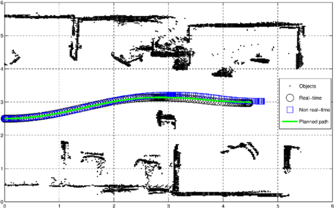
Actual actuation results in real time and non-real time

From these results, we can see that the proposed trajectory generation method can show sampling time uniformity and the ability to follow a path based on a Bezier curve with high curvature. Moreover, the convolution operator provides assurance in satisfying the physical limitations of the mobile robot. Implementation in a real-time operating system is also required to minimize the processing delay between tasks, which causes positional error during practical robot navigation.

6. Conclusion

In this paper, a practical joint-space trajectory generation method was proposed to manage the physical limitations of a mobile robot while considering the geometrical constraints of a path with high curvature.

A velocity profile generation technique that considers the acceleration limitations [10, 14] of the mobile robot does not consider other physical constraints such as maximum velocity and jerk, produces non-uniform sampling time and shows inability to discontinue at the junctions of consecutive paths. To address the drawbacks of the previous study, we present a convolution-based approach based on our previous research in [15], which considers the heading angles of a path based on a Bezier curve. This approach was able to produce a velocity profile that can manage the drawbacks of the preceding study; however, it also demonstrated an inability to follow a curved path with high curvature turning points in periodic sampling time.

For the general problem of generating a trajectory where the mobile robot manages the geometrical limitations present in a high curvature path while managing its physical limitations, the proposed method implements an adaptation of linear interpolation to the convolution-based velocity in order to generate central velocity commands that conciliate all the limitations of the previous methods.

In comparison with the preceding studies, numerical simulation results show distinct advantages in periodicity and time optimality by tracking the planned path with high accuracy at the fastest total travelling time.

The proposed approach was also a verified experimental example on a two-wheeled mobile robot driven with joint-space velocities in real-time control. The proposed trajectory generation technique was able to produce velocity commands to track a planned path based on a Bezier curve with high curvature while satisfying the physical limitations of the mobile robot and the geometrical constraints present along the planned path.

Footnotes

7. Acknowledgements

This work was supported by the Human Resources Development of the Korea Institute of Energy Technology Evaluation and Planning (KETEP) grant funded by the Korean government Ministry of Trade, Industry and Energy (NO. 20154030200720) and by the MOTIE (Ministry of Trade, Industry and Energy) and the KIAT (Korea Institute for Advancement of Technology) through the Industry Convergence/Connected for Creative Robot Human Resource Development (N0001126).

References

Brezak

Petrović

. Time-optimal trajectory planning along predefined path for mobile robots with velocity and acceleration constraints. In: Proceedings of the IEEE/ASME International Conference on Advanced Intelligent Mechatronics; 3–7 July 2011; Budapest, p. 942–947

Rodriguez-Seda

Tang

Spong

Stipanovic

. Trajectory tracking with collision avoidance for nonholonomic vehicles with acceleration constraints and limited sensing. The International Journal of Robotics Research. 2014;33(12):1569–1592

Bogue

. Robots for space exploration. Industrial Robot: An International Journal. 2012;39(4):323–328

Oustaloup

Orsoni

Melchior

Linares

. Path planning by fractional differentiation. Robotica. 2003;21(1):59–69

Kodagoda

Sehestedt

Dissanayake

. Socially aware path planning for mobile robots. Robotica. 2014;FirstView:1–14

Red

. A joint trajectory generator for motion recovery. Robotica. 2003;21(2):185–191

Dyllong

Visioli

. Planning and real-time modifications of a trajectory using spline techniques. Robotica. 2003;21(5):475–482

Fahimi

Van Kleeck

. Alternative trajectory-tracking control approach for marine surface vehicles with experimental verification. Robotica. 2013;31(1):25–33

Han

Choi

Lee

. A precise curved motion planning for a differential driving mobile robot. Mechatronics. 2008;18(9):459–528

10.

Lepetič

Klančar

Škrjanc

Matko

Potočnik

. Time optimal path planning considering acceleration limits. Robotics and Automation Systems. 2003;45(3–4):199–210

11.

Koh

Cho

. A path tracking control system for autonomous mobile robots: An experimental investigation. Mechatronics. 1994;4(8):799–820

12.

Liang

Liu

Hung

Chang

. Practical and flexible path planning for car-like mobile robot using maximal-curvature cubic spiral. Robotics and Automation Systems. 2005;52(4):312–335

13.

Yang

Jung

Sukkarieh

. Continuous curvature path-smoothing algorithm using cubic Bezier spiral curves for non-holonomic robots. Advanced Robotics. 2013;27(4):247–258

14.

Jolly

Sreerama-Kumar

Vijayakumar

. A Bezier curve based path planning in a multi-agent robot soccer system without violating the acceleration limits. Robotics and Automation Systems. 2009;57(1):23–33

15.

Yang

Choi

. Smooth trajectory planning along Bezier curve for mobile robots with velocity constraints. International Journal of Control and Automation. 2013;6(2):225–234

16.

Lee

Kim

Choi

. Convolution-based trajectory generation methods using physical system limits. ASME, Journal of Dynamic Systems, Measurement, and Control. 2013;135(1):1–8

17.

Zeng

Bone

. Mobile robot navigation for moving obstacles with unpredictable direction changes, including humans. Advanced Robotics. 2012;26(16):1841–1862

18.

Bronstein

Koren

. Real-time obstacle avoidance for fast mobile robots. IEEE Transactions on Systems, Man, and Cybernetics. 1989;19(5):1179–1187

19.

Simmons

. The curvature-velocity method for local obstacle avoidance. In: Proceedings of the 1996 IEEE International Conference on Robotics and Automation; 22–28 April 1996; Minneapolis, MN. p. 3375–3382

20.

Fernández

Sanz

Benayas

Diéguez

. Improving collision avoidance for mobile robots in partially known environments: the beam curvature method. Robotics and Automation Systems. 2004;6(4):205–219

21.

Borenstein

. Obstacle avoidance with ultrasonic sensors. IEEE Journal of Robotics and Automation. 1988;4(2):213–218

22.

Chakravarthy

. Obstacle avoidance in a dynamic environment: a collision cone approach. IEEE Transactions on Systems, Man, and Cybernetics. 1998;28(5):562–574

23.

Yang

Choi

. Joint-space trajectory planning considering physical limits with convolution operator for mobile robots. International Journal of Digital Content Technology and its Applications. 2013;7(11):248–257

24.

Choi

Shin

Park

Gerald

. Realtime control architecture using Xenomai for intelligent service robot in USN environment. Journal of Intelligent Service Robotics. 2009;2(2):139–151

25.

Jia

Yang

. LRF-based data processing algorithm for map building of mobile robot. In: Proceedings of the 2010 IEEE International Conference on Information and Automation; 20–23 June 2010; Harbin. p. 1924–1929

26.

Corregedor

Meyer

Plessis

. Design principles for 2D local mapping using a laser range finder. In: Proceedings of the 2011 IEEE AFRICON; 13–15 September 2011; Livingstone. p. 1–6

A Practical Joint-Space Trajectory Generation Method Based on Convolution in Real-Time Control

Abstract

Keywords

1. Introduction

2. Convolution-based Trajectory Generation

3. Path Planning Based on a Bezier Curve

4. Convolution-based Trajectory along a Bezier Curve

4.1. Smooth trajectory generation

4.2. Obstacle avoidance

4.3. High curvature trajectory generation

4.4. Joint-space velocities

5. Examples

5.1. Simulation example

5.2. Experimental example and results

6. Conclusion

Footnotes

7. Acknowledgements

References