A Control of Collision and Deadlock Avoidance for Automated Guided Vehicles with a Fault-Tolerance Capability

Abstract

Based on a novel discrete-event zone-control model, in our previous papers [1, 2], we presented a time-efficient traffic control for automated guided vehicle (AGV) systems to exclude inter-vehicle collisions and system deadlocks, together with a case study on container terminals. The traffic control allows each vehicle in an AGV system to freely choose its routes for any finite sequence of zone-to-zone transportation tasks and the routes can be constructed in an online fashion. In this paper, we extended our previous results with two practical goals: (1) to increase the utilization of the workspace area by reducing the minimally allowed area of each zone; (2) to avoid vehicle collisions and deadlocks with the occurrence of vehicle breakdowns. To achieve the first goal, we include one extra vehicle event that allows each vehicle to probe further ahead while it is moving on the guide-path. This leads to an extension of our previous discrete-event model and traffic control rules, which are presented in the first part of the paper. The second part of the paper concerns the second goal, for which an emergency traffic control scheme is designed as supplementary to the normal traffic control rules. As in our previous papers, the improved model and traffic control are applied to a simulation of quayside container transshipment at container terminals; our simulation results are compared with those from two interesting works in the literature.

1. Introduction

Automated guided vehicles (AGVs) are used as a transportation means in many industrial fields. Taking advantage of their flexibility in routing and scaling, AGV systems were traditionally employed in automated manufacturing systems (AMSs) as material handling systems (MHSs) to transport pieces or parts among various workstations. Recently, AGV systems have extended their popularity to other applications, such as material transportation in warehouses and container transshipment at container terminals. See, e.g., [3, 4] for comprehensive surveys of the research on the design of AGV systems.

As there are normally multiple vehicles in AGV systems, traffic control is necessary to resolve motion conflicts among the vehicles. In particular, vehicle collisions and deadlocks should be prevented to avoid substantial production interruptions. Furthermore, for an AGV system with a large number of vehicles in some applications, effective and efficient traffic control is also important to achieve desirable system performance (see, e.g., [5] for a list of performance measures).

Traditionally and still currently, AGVs move along a predefined guide-path (wired, magnetic, etc.) system connecting key locations in the workspace, which eases the motion control and guidance of the vehicles, yet sets limitations on the flexibility and scalability of the system. The literature and industrial practice have witnessed a growing interest in developing free-ranging AGV systems, in which the vehicles can choose any possible path to move between two locations. This type of system is expected by some researchers to provide shorter transportation distances (via free routing), better utilization of the workspace and more flexible deadlock and congestion avoidance mechanisms. However, performance comparisons between free-ranging AGV systems and those with a fixed guide-path are very rarely seen [6]; besides, it seems that convincing conclusions have not yet been drawn on which type would perform better with dense vehicles (i.e., a large number of vehicles in a limited area). In this paper, we choose to focus on a study of AGV systems with a fixed guide-path.

Several types of flow topologies/configurations have been proposed and investigated for the guide-path of the AGV systems. Each of them has its pros and cons and should be chosen based on specific applications. All the flow configurations contain a collections of lanes, or sequences or path segments (either unidirectional or bidirectional), connecting machines, work stations, pick-up and delivery points or other fixed infrastructures. In what is called conventional configuration, lanes can intersect each other like in a normal guide-path. In single loop configuration, AGVs travel in a fixed (usually unidirectional) loop. The advantage is that the traffic is easy to control; however, each vehicle has to travel the complete loop to visit the same point again and a vehicle breakdown can block the entire system. The tandem configuration consists of non-overlapping single loops and uses transfer stations to move materials from one loop to another. As with the single loop layout, it also requires little or even no traffic control (if only one vehicle serves one loop); hence, some researchers concluded that tandem layout performs better in large systems (see, e.g., [7]). However, any single loop is a bottleneck to the whole system; besides, extra space and equipment are required for the transfer stations. Lastly, similar to a tandem configuration, a segmented flow configuration contains one or more zones, each of which is divided into non-overlapping segments served by a single vehicle. Some papers also showed good performance (see, e.g., [8]) by using this type of guide-path, but it shares the same drawbacks as with the tandem configuration. The reader is referred to [3, 4] for more details on the classification and design of the guide-path. This paper discusses the traffic control of AGV systems with conventional guide-path (as aforementioned, the traffic control of the other types of guide-path configurations is heavily reduced or even fully removed).

The most popular traffic control strategy for AGV systems is called zone-control (see [9]), in which lanes in the guide-path are composed of a number of zones. By this strategy, inter-vehicle collision avoidance becomes straightforward by only allowing one vehicle to visit one zone at a time. A key traffic control issue is then to keep the vehicles away from deadlocks that may be caused by the vehicles' competition for the occupation of the zones.

Historically, the study on deadlock problems started in the development of operating systems [10, 11] and database systems [12] in computer science. In general, three strategies have been employed to address deadlocks: deadlock prevention, deadlock avoidance and deadlock detection and resolution [12]. The goal of deadlock prevention is to design rules such that any deadlock is precluded before all processes set off. In a deadlock avoidance strategy, online control is adopted such that a resource is allocated to a process only if a deadlock will not be introduced. Lastly, a deadlock detection and resolution strategy allows deadlock to happen. When a deadlock is detected, certain online rules are used to resolve the deadlock and recover the system. During the past two decades, deadlock problems have been attracting intensive research effort for the flexible manufacturing systems (FMSs), in which AGV systems play an important part. In particular, [13–18] are among many other works that investigate deadlock avoidance using Petri net formalism. The proposed methods either exclude the occurrence of deadlocks by preventing some necessary conditions, or detect and resolve deadlocks when they actually take place [19]. [20] and [21] proposed deadlock avoidance policies based on the graphic characterization of deadlocks and so-called restricted deadlocks. In [22], a variation of the Banker's algorithm was developed, which prevents deadlocks by allowing only “ordered” vehicle mission trips. The conservativeness of this algorithm is somewhat reduced in [23] and [24] at the cost of higher complexity. There are some other methods existing in the literature. [25] provides a generalized algebraic deadlock avoidance policy that ensures the absence of deadlocks by restricting the operation of the system in a subspace satisfying a set of linear inequalities. Using a graph theoretic approach, [26] presented a deadlock avoidance algorithm that consists of a quasi two-step resource allocation policy and a cyclic deadlock detection procedure. [27] offers a logic-algebraic approach for deadlock prevention by solving a constraint satisfaction problem. In addition, many works have been dedicated to guaranteeing deadlock avoidance by using smart routing algorithms (sometimes called conflict-free routing) [28–31, 24]. Note also that recent years have witnessed an increasing research interest in traffic control problems for the AGV systems at automated container terminals, as the volume of goods transported via sea ports has soared in booming international trade. [32] presented several procedures to detect and recover from deadlocks caused by the interaction between the AGV system and other container handling equipment systems. [33] renders a path reservation method to prevent in advance the deadlocks and collisions of AGVs. [34] suggested a traffic control approach based on the concept of “semaphore” borrowed from computer science. In addition, inspired by [35], the work of [36] and later [1] (with core models and algorithms reformed in [2]) showed deadlock detection and avoidance schemes involving some online cyclic deadlock checking procedures for a unidirectional guide-path system.

As pointed out by [3] and [36], dealing with deadlock avoidance for relatively large AGV systems (a large number of AGVs and/or zones) is quite challenging. In fact, this makes most of the existing algorithms either too conservative with acceptable complexities, or too computationally expensive under the pursuit of least restriction. Very recently, there have been some research activities aiming at maximally permissive deadlock avoidance algorithms with complexity concerns by using the resource allocation system theory [37] and Petri net formalism [38]. However, it seems that there is still quite some distance from the current status of the development to the practical applications of these optimal algorithms for large-scale AGV systems (with tens or even hundreds of vehicles). To the authors' best knowledge, the deadlock avoidance algorithms proposed in [35, 36, 1, 2] have the smallest computational complexities, which only quadratically increase with the number of vehicles. Note that the small complexities of these algorithms partially come from their limited applicability to guide-path systems with only unidirectional lanes. However, for large-scale AGV systems, the potential room for performance improvement using bidirectional guide-path systems shrinks with increasing vehicle interferences ([39, 29]) and comes with a sharp rise of complexity of traffic management. Furthermore, one also notes that the traffic control with bidirectional guide-path in general depends on the scheduling and routing of the vehicles, whereas the traffic control algorithm proposed in our previous work [2] has been proven able to avoid deadlocks with no restrictions to routing of the vehicles, as long as each vehicle visits a finite sequence of zones from its initial location to a depot (where it can stay without blocking other vehicles). This free-routing property is definitely a big advantage in achieving high system performance. Note also that among the algorithms proposed in [35, 36, 2], only the one in [2] is provably correct in guaranteeing the absence of deadlocks with the help of a formal event-based modelling. (The problems with the algorithms in [35] have been pointed out in [21]; in [36] the authors did not obtain a complete solution for what they call “multi-cycle deadlocks”.)

Failures can degrade the performance of or even paralyse an industrial system. Fault-tolerance is, therefore, one of the key properties that make an industrial system practically useful. In the literature of deadlock avoidance, several studies have been made on fault-tolerant deadlock avoidance for some types of automated manufacturing systems modelled by Petri nets [40, 41]. In addition, some fault-tolerant routing algorithms have been developed for computer networks and for communication subsystems on integrated circuits [42, 43]. For deadlock avoidance for AGV systems, however, there is hardly any existing work that has the management of vehicle faults as a focus. In principle, for the AGV systems with free-ranging vehicles, vehicle breakdowns may be handled by letting the other (healthy) vehicles view the faulty vehicles as obstacles that can be steered clear of with their (i.e., the healthy vehicles') built-in obstacle avoidance algorithms. However, detailed discussion and formal proofs for collision and deadlock avoidance in this direction are rarely seen in the literature. For the AGV systems with guide-paths, vehicle breakdowns can be catastrophic for certain types of configuration of guide-path. For example, in the single loop configuration, where AGVs travel in a fixed (usually unidirectional) loop, a vehicle breakdown can block the whole system; in the tandem configuration, which consists of non-overlapping single loops, each single loop is a bottleneck to the entire system; the same problem can happen to the segmented flow configuration with each of the non-overlapping segments served by a single vehicle. For other types of guide-path, the AGV system might still be able to function after some vehicle breakdowns; however, a partial or complete re-dispatching, re-scheduling and/or re-rerouting may be necessary to ensure acceptable system performance. With most existing deadlock avoidance approaches, the adjustment has to be responsible for the deadlock avoidance of the AGV system as well.

In this paper, we follow the line of development in [1, 2] to design traffic control algorithms for AGV systems that guarantee the avoidance of collision and deadlocks with full freedom of routing. We have two specific goals in mind: (1) increase the utilization of the workspace area by reducing the minimally allowed area of each zone; and (2) design an emergency traffic control scheme to avoid vehicle collisions and deadlocks with the presence of vehicle breakdowns. Both these goals are motivated by practical concerns from general applications. The key to the realization of the first goal is adding one extra event to the event-based model previously presented in [2]. The triggering of this event allows a vehicle to probe the availability of one more zone ahead on its path than before. For applications with a large number of zones, this can lead to substantial saving of space. The second goal is clearly designed to improve the robustness of traffic control to emergency situations, which is rarely addressed in literature, at least in a formal manner. Note that the achievement of the first goal also gives some leeway to that of the second, for which we enlarge the first zone of each lane so that it contains some extra space that can be split out, if needed, into a buffer zone when a vehicle breakdown occurs.

The paper is organized as follows: the extended discrete-event zone-control model is introduced in Section 2. The traffic control rules that ensure the avoidance of collision and deadlocks in a fault-free situation are presented in Section 3. A performance study of an AGV system incorporating the proposed traffic control is mentioned in Section 4. The emergency traffic control rules that guarantee the avoidance of collision and deadlocks with vehicle breakdowns are presented in Section 5. Concluding remarks are given in Section 6. All the technical proofs are included in the appendix of the paper.

2. Zone-control Modelling

In this section, we present the zone-control model that defines the structure of the guide-path ¹ and the event-driven vehicle behaviour. In particular, at the end of Section 2.2, we will show how our first goal of increasing the utilization of the workspace area is achieved by this extension to our previous work [2].

2.1. Building blocks of the zone-based guide-path

The guide-path contains lanes, crossings and depots. Lanes are composed of zones and each depot is a (special) zone. For any assigned transportation task, a vehicle does nothing but move from one zone to another. Some of the content in this section can be found in [2], but is still presented here for completeness.

2.1.1. Lane and zone

A lane is a finite sequence of zones. Vehicles moving in a lane must visit the zones according to their order in the sequence. In the general discussion that follows, we assume that there are M, $M\in \mathbb{N}$ (ℕ denotes the set of natural numbers), lanes in the network and the lane i has m_i, $m_i\in \mathbb{N}$ , zones. In addition, we use $c_k^i$ to denote the k th zone of the lane i. In particular, we call the first zone and the last zone of a lane the starting zone (SZ) and ending zone (EZ) of the lane, respectively. In practice, a zone should be large enough to accommodate at least one vehicle.

A depot is a zone that can accommodate any number of vehicles. We emphasize that a depot is not a zone of any lane; or, in other words, any zone on each lane is a non-depot zone. Each depot is affiliated with at least one entry-lane and one exit-lane. Physically, an entry-lane (resp. exit-lane) of a depot is a lane that allows a vehicle to move inwards (or outwards) from the depot.

We use $\mathcal{C}$ to denote the set of all zones in the guide-path.

2.1.2. Crossing

A crossing is physically a junction that joins multiple lanes. Specifically, crossing i is affiliated with a set of in-lanes, denoted by ℐ_i and a set of out-lanes, denoted by ${\mathcal{O}}_i$ . Each lane in ℐ_i has a (non-empty) set of neighbouring lanes, which is a subset of ${\mathcal{O}}_i$ . Vehicles can move from an in-lane of a crossing onto any of its neighbouring lanes by passing the crossing. A zone pair $(c_1\mathrm{,}{c}_2)$ is thus called a crossing-passing zone pair of crossing i if c₁ is the EZ of a lane j in ℐ_i and c₂ is the SZ of a neighbouring lane of the lane j. We denote the collection of all the crossing-passing zone pairs of crossing i by ℛ_i (Hence ℛ_i characterizes all possible ways of passing the crossing i). For each zone pair $(c_1\mathrm{,}{c}_2)\in {ℛ}_i$ , there is a subset (maybe empty) of ℛ_i, denoted by ${\mathcal{X}}_i(c_1\mathrm{,}{c}_2)$ , in which the zone pairs are called the conflicting crossing-passing zone pairs of $(c_1\mathrm{,}{c}_2)$ at the crossing i. Physically, if $(c_3\mathrm{,}{c}_4)\in {\mathcal{X}}_i(c_1\mathrm{,}{c}_2)$ , then a vehicle passing the crossing i by moving from c₁ to c₂ can collide with another vehicle passing the same crossing by moving from c₃ to c₄. For this reason, for any crossing i, it is considered that $(c_3\mathrm{,}{c}_4)\in {\mathcal{X}}_i(c_1\mathrm{,}{c}_2)$ if and only if $(c_1\mathrm{,}{c}_2)\in {\mathcal{X}}_i(c_3\mathrm{,}{c}_4)$ . For each crossing i, we call the set of EZs of all its in-lanes at-crossing zones of the crossing i. A zone is called an off-crossing zone if it is not an at-crossing zone of any crossing.

2.1.3. Assumptions on the guide-path

Upon the layout of the guide-path, we impose the following guide-path layout assumptions:

• (A1) $c_{k_1}^{i_1}\ne c_{k_2}^{i_2}$ if either $i_1\ne i_2$ or $k_1\ne k_2$ .

• (A2) Each lane is either an in-lane of a unique crossing or an entry-lane of a unique depot, but cannot be both.

• (A3) Each lane can be either an exit-lane of at most one depot or an out-lane of at most one crossing, but cannot be both the exit-lane of a depot and the out-lane of a crossing.

• (A4) Each lane has at least two zones, with the following exceptions (where it can have only one zone): (i) it is an entry- or exit-lane of a depot, (ii) it is an out-lane of a crossing and there is at most one in-lane of the crossing that has it as a neighbouring lane and the in-lane is different from it and (iii) it is neither an out-lane of a crossing nor an exit-lane of a depot.

Figure 1 illustrates an example of such a guide-path.

Figure 1.

A guide-path: the dashed arrows indicate the order of zones in the corresponding lanes; the boxes with crosses denote the crossings. For the crossing i, ${ℛ}_i=\{(c_1\mathrm{,}{c}_2)\mathrm{,}(c_3\mathrm{,}{c}_4)\mathrm{,}(c_5\mathrm{,}{c}_6)\}$ , ${\mathcal{X}}_i(c_1\mathrm{,}{c}_2)=\{(c_3\mathrm{,}{c}_4)\mathrm{,}(c_5\mathrm{,}{c}_6)\}$ . Disks with numbers represent vehicles.

In the above assumptions, (A1) says that each lane neither self-intersects nor intersects with any other lane; (A2) implies that each lane connects to a depot or another lane (via a crossing); (A4) is key to the deadlock avoidance by the traffic control presented later. In addition, note that (A3) does not exclude the case that a lane is neither an exit-lane of a depot nor an out-lane of a crossing (e.g., the lane depicted at the top left corner of Figure 1).

2.1.4. Neighbouring zone

It is important to know, when a vehicle is in a zone, which zones the vehicle can move into next. For this purpose we define the concept neighbouring zone, which intuitively follows the definitions of lanes and depots. The set of neighbouring zones of each depot consists of the SZs of all its exit-lanes. The neighbouring zone of a non-EZ zone $c_k^i$ , $i\in \{\mathrm{1,2,}\cdots \mathrm{,}M\}$ , $k\in \{\mathrm{1,2,}\cdots \mathrm{,}{m}_i-1\}$ , is $c_{k+1}^i$ . The neighbouring zone of the EZ of any entry-lane of a depot is the depot. The neighbouring zones of the EZ of an in-lane of a crossing are the SZs of its neighbouring lanes ² . We use ϒ_c to denote the set of neighbouring zones of zone c. In addition, for any $c\in \mathcal{C}$ , define ${\tilde{\Upsilon }}_c=\{c^{*}\in \mathcal{C}:c\in {\Upsilon }_{c^{*}}\}$ .

2.2. Vehicle state and event

The state of a vehicle indicates its current location and intention of movement with respect to the guide-path. Each vehicle can have three types of states, as follows:

1. in c₁ with the next zone c₂, denoted by $(c_1\mathrm{,}{c}_1\mathrm{,}{c}_2)$ ;

2. moving from c₁ to c₂, denoted by $(c_1\mathrm{,}{c}_2\mathrm{,}{c}_2)$ ;

3. moving from c₁ to c₃ via c₂, denoted by $(c_1\mathrm{,}{c}_2\mathrm{,}{c}_3)$ ;

where c₁ can be any zone in $\mathcal{C}$ , c₂ is one of the neighbouring zones of c₁ (i.e., $c_2\in {\Upsilon }_{c_1}$ ) and c₃ is a neighbouring zone of c₂ but different from c₁. In all three cases, c₁ and c₂ are called, respectively, the current zone and the next zone of the vehicle. From an implementation point of view, the body of a vehicle is supposed to be entirely inside its current zone in case (1) and may span across its current zone and the next zone in cases (2) and (3).

To ease the presentation, we define three sets that collect all possible vehicle states in each of the above three types:

${\mathcal{S}}_1=\{(c_1\mathrm{,}{c}_1\mathrm{,}{c}_2)\in {\mathcal{C}}^3:c_2\in {\Upsilon }_{c_1}\}\mathrm{,}$

${\mathcal{S}}_2=\{(c_1\mathrm{,}{c}_2\mathrm{,}{c}_2)\in {\mathcal{C}}^3:c_2\in {\Upsilon }_{c_1}\}\mathrm{,}$

${\mathcal{S}}_3=\{(c_1\mathrm{,}{c}_2\mathrm{,}{c}_3)\in {\mathcal{C}}^3:c_2\in {\Upsilon }_{c_1}\mathrm{,}{c}_3\in {\Upsilon }_{c_2}\backslash \{c_1\left\}\right\}\mathrm{.}$

In addition, we let $\mathcal{S}$ be the union of ${\mathcal{S}}_1$ , ${\mathcal{S}}_2$ and ${\mathcal{S}}_3$ . Note that, by Lemma 2 (see Section A.1), c₁, c₂ and c₃ are distinct in the definitions of ${\mathcal{S}}_1$ , ${\mathcal{S}}_2$ and ${\mathcal{S}}_3$ and thus the three sets are disjoint. For any $s\in \mathcal{S}$ , we will sometimes use $s_1\mathrm{,}{s}_2\mathrm{,}{s}_3$ to denote its first, second and third elements respectively.

Each vehicle has an initial state representing its beginning location and intention of movement. When the system is running, the state of each vehicle will change only at the occurrence of events. In other words, an event is responsible for a state transition that maps a vehicle state to another. There are three events that vehicles trigger for their normal operations: “leave”, “arrive” and “go ahead” ³ . To simplify the presentation, we use LEA, ARR and GOA to denote the three events respectively. At any point in time, each vehicle can trigger at most one event; the following rules prescribe how the three events change the state (denoted by s) of a vehicle:

• if $s=(c_1\mathrm{,}{c}_1\mathrm{,}{c}_2)\in {\mathcal{S}}_1$ , then the only feasible event for s is an LEA, which changes s to $(c_1\mathrm{,}{c}_2\mathrm{,}{c}_2)\in {\mathcal{S}}_2$ ;

• if $s=(c_1\mathrm{,}{c}_2\mathrm{,}{c}_2)\in {\mathcal{S}}_2$ , then both an ARR and a GOA are feasible for s: (i) an ARR changes s to $(c_2\mathrm{,}{c}_2\mathrm{,}{c}_3)\in {\mathcal{S}}_1$ , where c₃ can be any zone in ${\Upsilon }_{c_2}$ ; (ii) a GOA changes s to $(c_1\mathrm{,}{c}_2\mathrm{,}{c}_3)\in {\mathcal{S}}_3$ , where c₃ can be any zone in ${\Upsilon }_{c_2}\backslash \left\{c_1\right\}$ ;

• if $s=(c_1\mathrm{,}{c}_2\mathrm{,}{c}_3)\in {\mathcal{S}}_3$ , then the only feasible event for s is an ARR, which changes s to $(c_2\mathrm{,}{c}_3\mathrm{,}{c}_3)\in {\mathcal{S}}_2$ .

Note that the ARR and GOA in (b) are the events that involve new zones in the state transitions and thus directly relate to the implementation of the routes of the vehicles.

The state transitions by the three events are illustrated in Figure 2. In a less formal and much simpler way, we sometimes say that:

Figure 2.

The state transitions by the three events

• in (a), the vehicle leaves c₁ by the LEA;

• in (b), the vehicle goes ahead to pass c₂ by the GOA;

• in (b) and (c), the vehicle arrives at c₂ by the ARRs.

Here we give a simple example of how each vehicle is supposed to utilize these events to change its state while moving on the guide-path. Consider a vehicle that has the state $(c_1\mathrm{,}{c}_1\mathrm{,}{c}_2)$ (i.e., it is in the zone c₁) and wants to be in $c_3\in {\Upsilon }_{c_2}$ . This can be achieved by first leaving c₁, then going ahead to pass c₂, arrive at c₂ and finally arrive at c₃ (i.e., by the event sequence LEA→GOA→ARR→ARR ⁴ ).

We should emphasize that, although an event is feasible for a particular vehicle state, it does not mean that the event is always allowed to occur for the state. The traffic rules that will be presented in the following section are used to permit or inhibit events such that vehicle collisions are avoided and system deadlock can never happen. An interesting point to mention here is that an ARR is always allowed to occur by the traffic rules. Thus, the freedom in selecting the zone c₃ with the ARR in case (b) allows a vehicle to alter its route even if it has been predefined, or establish it online in an incremental fashion: a vehicle only needs to pick c₃, the succeeding zone on its route, before it arrives at c₂. The selection of the zone c₃ with the GOA event in (b) is also free; the only difference is that a GOA event can be prohibited by the traffic rules. Later on, we will see that there are no restrictions imposed on a route assignment before each transportation trip either. This free-routing property is a distinct advantage of the proposed traffic control.

From another perspective, considering the zones as resources that vehicles need to take up for their transportation trips, the above events, together with the traffic control, can also be seen to dictate the resource allocation for the overall system (in section 2.3, we will see that this is directly related to the states of zones). Specifically, in (a) the vehicle is allocated c₂ by the LEA, yet has not released c₁; by the GOA in (b) the vehicle is allocated c₃, yet has released neither c₁ nor c₂; the ARRs in both (b) and (c) release the zone c₁. Because of the last point, it is required that the vehicle has already physically moved completely out of c₁ and is inside c₂ when the ARRs are triggered. In addition, for high system performance it is good to have the ARRs triggered (so that c₁ is released) immediately after the vehicle fully enters c₂. From case (c), we see that this implies that the vehicle is not physically occupying the zone c₃ when its state is $(c_1\mathrm{,}{c}_2\mathrm{,}{c}_3)$ , as the zone c₂ is large enough to accommodate the entire body of the vehicle.

One may notice that, compared with the discrete-event model presented in our previous work [2] (or in [1] in a different form) the driving idea behind all the modifications is the addition of the event GOA, which extends the behaviour of the vehicles. In fact, previously only two types of vehicle states were defined, i.e., the states in ${\mathcal{S}}_1$ and ${\mathcal{S}}_2$ and the event-driven state transitions shown in the dashed box in Figure 2.

Let us now explain the improvement brought about by the present and generalized model by using a walk-through of a typical scenario in which a vehicle tries to pass a zone. Consider a vehicle trying to pass a zone c₂ with its current state $(c_1\mathrm{,}{c}_2\mathrm{,}{c}_2)$ and suppose it knows the next zone (after passing c₂) on its route is $c_3\in {\Upsilon }_{c_2}$ . What will happen with the previous model is the following: the vehicle will have to trigger an ARR to arrive at c₂ first (c₁ will then be released). As stated above, this requires the body of the vehicle to be fully inside c₂. The vehicle will then try to trigger an LEA to leave c₂ (so that its state can be changed to $(c_2\mathrm{,}{c}_3\mathrm{,}{c}_3)$ ). If the LEA is permitted (by the traffic control), the vehicle will keep its speed and move on, passing c₂; otherwise, it has to break and make a full stop with its body still completely inside c₂. Clearly, we need the length of zone c₂ to be at least $L_{vehicle}+L_{break}$ in case the LEA is denied, where $L_{vehicle}$ is the length of the vehicle and $L_{break}$ is the distance for the vehicle to make a full stop from its maximum speed. Now, for the same scenario, let us follow the vehicle's behaviour in the framework of the present model. First, the vehicle will try to trigger a GOA, which changes its state to $(c_1\mathrm{,}{c}_2\mathrm{,}{c}_3)$ . Importantly, note that the vehicle can do this even before physically entering the zone c₂. If the GOA is permitted (the zone c₃ is then allocated to the vehicle), it will move on, passing c₂; otherwise, it will need to break and fully stop inside c₂. It is easily seen that in this case the length of c₂ will need only to be larger than $\text{max}\left\{L_{vehicle}\mathrm{,}{L}_{break}\right\}$ . For a guide-path with a large number of zones, this improvement can be substantial if the breaking distance $L_{break}$ is not negligible with respect to $L_{vehicle}$ (e.g., with the container-carrying vehicles at container terminals). With a closer look, one may notice that the saving of required space as the vehicle passes c₂ is essentially due to the early can-pass probing via the trial of the GOA.

2.3. Zone states

Before closing this section, we introduce some properties of the zones that are directly related to the states of vehicles.

Each zone can have two states: “occupied” and “available”. In particular, a depot is always available. A non-depot zone is occupied if it is allocated to a vehicle; it should not be allocated to another one before being released. Put more formally, a non-depot zone is said to be occupied by a vehicle, with state s, when (1) it is the current zone of the vehicle if $s\in {\mathcal{S}}_1$ ; or (2) it appears in the expression of s if $s\in {\mathcal{S}}_2\cup {\mathcal{S}}_3$ . A non-depot zone is said to be occupied if it is occupied by at least one vehicle. A non-depot zone is available if it is not occupied. It is obvious that the states of zones change only at the occurrence of vehicle events. It is part of the responsibility of the traffic control to ensure that a zone is occupied by at most one vehicle, so that vehicle collisions are avoided.

To ease our presentation, we sometimes use colours to represent different statuses (not states) of the zones. Specifically,

• Any zone c is white ⇔c is available;

• Any non-depot zone c is black ⇔c is occupied by only one vehicle with the state either $(c\mathrm{,}c\mathrm{,}{c}^{*})\in {\mathcal{S}}_1$ , $(c^{*}\mathrm{,}c\mathrm{,}c)\in {\mathcal{S}}_2$ or $(c^{*}\mathrm{,}{c}^{**}\mathrm{,}c)\in {\mathcal{S}}_3$ ;

• Any non-depot zone c is grey ⇔c is occupied by only one vehicle with the state either $(c\mathrm{,}{c}^{*}\mathrm{,}{c}^{*})\in {\mathcal{S}}_2$ , $(c\mathrm{,}{c}^{*}\mathrm{,}{c}^{**})\in {\mathcal{S}}_3$ or $(c^{*}\mathrm{,}c\mathrm{,}{c}^{**})\in {\mathcal{S}}_3$ ;

where, in (b) and (c), $c^{*}$ and $c^{**}$ can be any zones that make sense.

One can see that a zone is black if it is occupied by a vehicle that is either in the zone or will be able to be in the zone after triggering one or two ARRs (recall that ARRs are always allowed). A zone is grey if it is occupied by a vehicle that will be able to release the zone after triggering a couple of ARRs.

It is easy to show that, if each non-depot zone is occupied by at most one vehicle, then any zone must be either white (when available), black or grey (when occupied).

Finally, we say that a vehicle starts occupying a zone by an event if the zone was not occupied by the vehicle before the state transition, caused by the event, but is occupied by the vehicle afterwards. It can be shown that such an event can be either an LEA or a GOA but not an ARR (see Lemma 4 in Section A.1).

3. Traffic Control

In this section, we will propose a traffic control system that guarantees the absence of (inter-vehicle) collisions and deadlocks. One may notice that the traffic control here is slightly more complex than that previously proposed in [1, 2], mainly due to the added event GOA and vehicle states in the set ${\mathcal{S}}_3$ . Basically, the traffic control permits a vehicle to trigger an ARR whenever it wishes to do so, but requires it to check with some specified traffic rules when it intends to trigger either an LEA or a GOA.

Since there are different traffic rules for different situations, we now introduce a classification of the LEA and GOA events. An LEA (or GOA) is called an off-crossing LEA (or off-crossing GOA) if it causes a vehicle to leave (GOA: go ahead to pass) an off-crossing zone; is called an at-crossing LEA (or at-crossing GOA) at a crossing if it causes a vehicle to leave (GOA: go ahead to pass) an at-crossing zone of the crossing. An event is called a crossing-passing event at a crossing if it is either an at-crossing LEA or an at-crossing GOA at the crossing. An LEA or GOA is called a depot-passing event at a depot if it causes a vehicle to either leave or go ahead to pass the depot. Clearly, a depot-passing event cannot be a crossing-passing event.

3.1. Inter-vehicle collision avoidance

The requirement for collision avoidance can be roughly stated as the following: first, any non-depot zone cannot be occupied by two or more vehicles at the same time. Second, it must be excluded that two vehicles are passing a crossing in a conflicting way or will be doing so due to the lack of further restrictions. More specifically, let s and $s^{\prime }$ be the states of two vehicles at the same time instant; the latter point is achieved for the crossing k if the following cases are prevented:

• (X1) $s\mathrm{,}{s}^{\prime }\in {\mathcal{S}}_2$ with $(s_1\mathrm{,}{s}_2)\in {\mathcal{X}}_k({s^{\prime }}_1\mathrm{,}{s^{\prime }}_2)$ ;

• (X2) $s\in {\mathcal{S}}_2$ , $s^{\prime }\in {\mathcal{S}}_3$ with either $(s_1\mathrm{,}{s}_2)\in {\mathcal{X}}_k({s^{\prime }}_1\mathrm{,}{s^{\prime }}_2)$ or $(s_1\mathrm{,}{s}_2)\in {\mathcal{X}}_k({s^{\prime }}_2\mathrm{,}{s^{\prime }}_3)$ ;

• (X3) $s\mathrm{,}{s}^{\prime }\in {\mathcal{S}}_3$ with one of the possibilities: $(s_1\mathrm{,}{s}_2)\in {\mathcal{X}}_k({s^{\prime }}_1\mathrm{,}{s^{\prime }}_2)$ , $(s_1\mathrm{,}{s}_2)\in {\mathcal{X}}_k({s^{\prime }}_2\mathrm{,}{s^{\prime }}_3)$ , $(s_2\mathrm{,}{s}_3)\in {\mathcal{X}}_k({s^{\prime }}_1\mathrm{,}{s^{\prime }}_2)$ , $(s_2\mathrm{,}{s}_3)\in {\mathcal{X}}_k({s^{\prime }}_2\mathrm{,}{s^{\prime }}_3)$ .

Case (X1) in fact reflects the motivation for defining the notation of conflicting crossing-passing zone pairs ${\mathcal{X}}_k$ (see Section 2). The reason for the inclusion of (X2) and (X3) is that a vehicle with the state $(s_1\mathrm{,}{s}_2\mathrm{,}{s}_3)\in {\mathcal{S}}_3$ is always allowed to trigger an ARR and change its state to $(s_2\mathrm{,}{s}_3\mathrm{,}{s}_3)\in {\mathcal{S}}_2$ . In all three cases above, we say that the state s conflicts with the state $s^{\prime }$ at crossing k. In summary, the AGV system is said to be free of collisions if both the following two conditions are satisfied:

• (C1) Each non-depot zone is occupied by at most one vehicle.

• (C2) The state of each vehicle does not conflict with that of any other at any crossing.

First, we need to prevent two vehicles leaving or going ahead to pass the same depot and start occupying the SZ of the same exit-lane of the depot simultaneously. For this purpose, the following Rule 1 is imposed:

Rule 1: For each depot, at most one vehicle is allowed to trigger a depot-passing event at the depot at any time.

Similarly, we also need to avoid two vehicles triggering at-crossing LEAs or GOAs at the same crossing to start occupying the SZ of the same out-lane of the crossing simultaneously. This gives ground to the following Rule 2:

Rule 2: For each crossing, at most one vehicle is allowed to trigger a crossing-passing event at the crossing at any time.

Rule 1 (or Rule 2) can be realized by requiring each vehicle to hold exclusively a local depot token (Rule 2: local crossing token) whenever triggering a depot-passing (Rule 2: crossing-passing) event at each depot (Rule 2: crossing). An example of such token assignment algorithms can be found in [1].

In addition, Rule 3 and Rule 4 below are used to make sure that a vehicle cannot start occupying a zone if the zone is occupied by another vehicle and/or doing so will give rise to two vehicles having conflicting states at a crossing.

Rule 3 (on off-crossing LEA and GOA): If a vehicle is in the state $s=(c_1\mathrm{,}{c}_1\mathrm{,}{c}_2)\in {\mathcal{S}}_1$ , where c₁ is an off-crossing zone, then an (off-crossing) LEA is allowed to be triggered and to change the state of the vehicle to $(c_1\mathrm{,}{c}_2\mathrm{,}{c}_2)$ if c₂ is available; if $s=(c_1\mathrm{,}{c}_2\mathrm{,}{c}_2)\in {\mathcal{S}}_2$ , where c₂ is an off-crossing zone, then an (off-crossing) GOA is allowed to be triggered and to change the state of the vehicle to $(c_1\mathrm{,}{c}_2\mathrm{,}{c}_3)$ if c₃ is available.

Rule 4 (on at-crossing LEA and GOA): If a vehicle is with the state $s=(c_1\mathrm{,}{c}_1\mathrm{,}{c}_2)\in {\mathcal{S}}_1$ , where c₁ is an at-crossing zone of crossing i, then an (at-crossing) LEA is allowed to be triggered and to change the state of the vehicle to $s^{\prime }=(c_1\mathrm{,}{c}_2\mathrm{,}{c}_2)$ if (1) c₂ is available and (2) there is no other vehicle having its state with $s^{\prime }$ at crossing i; if $s=(c_1\mathrm{,}{c}_2\mathrm{,}{c}_2)\in {\mathcal{S}}_2$ , where c₂ is an at-crossing zone of crossing i, then an (at-crossing) GOA is allowed to be triggered and to change the state to $s^{\prime }=(c_1\mathrm{,}{c}_2\mathrm{,}{c}_3)$ if (1) c₃ is available and (2) there is no other vehicle with its state conflicting with $s^{\prime }$ at crossing i.

It can be proved that traffic rules guarantee that an AGV system is free of collisions if the two conditions (C1) and (C2) are satisfied initially. We refer the interested reader to Section A.2.1 for a formal proof of the collision avoidance.

3.2. Deadlock avoidance

Abstracting from many applications, we may consider that each vehicle in an AGV system does nothing but visit a series of zones to transport things from assigned pick-up points to delivery points. In the framework of our event-driven model, to realize this a vehicle must trigger a sequence of events. We say that a vehicle is operational if it has the intention to trigger a new event in finite time; it is supposed that if a vehicle is not operational (and not faulty) it must be in a depot. Without loss of generality, we also assume that each vehicle is initially operational and terminates its operation after visiting a finite sequence of zones. It follows that each vehicle can terminate its operation after triggering finite events. In fact, if a vehicle triggers infinite events, one easily sees from Figure 2 that there must be infinite LEAs and/or infinite GOAs, which, by Lemma 4 (see Section A.1), implies that the vehicle would occupy an infinite sequence of zones.

We say that an operational vehicle is blocked if all feasible events for the state of the vehicle are not allowed to occur in finite time. Now we show that, if, at any time, at least one operational vehicle is not blocked, then all vehicles can successfully terminate their operations in finite time. By contradiction, suppose that there are some vehicles remaining operational all the time. Then, these vehicles would be able to trigger an infinite number of events, as at any time one of them is able to trigger an event in the finite future. This, however, implies that these vehicles can terminate their operations, since, as assumed, each operational vehicle can terminate its operation after triggering finite events.

This observation motivates us to give the definition of deadlock of the AGV system as follows: the AGV system has a deadlock if all operational vehicles are blocked. From the argument above, it is clear that every vehicle can terminate its operation if the AGV system is free of deadlocks (at all times).

Note that there is a special type of deadlock scenario, i.e., cyclic deadlocks: a group of operational vehicles $v_{i_1}\mathrm{,}{v}_{i_2}\mathrm{,}\cdots \mathrm{,}{v}_{i_m}$ , $m\ge 2$ , are respectively in m distinct zones $c_1\mathrm{,}{c}_2\mathrm{,}\cdots \mathrm{,}{c}_m$ , where $c_{j+1}$ is the next zone of $v_{i_j}$ for $j=\mathrm{1,2,}\cdots \mathrm{,}m-1$ and c₁ is the next zone of $v_{i_m}$ . In this case, by Rules 3 and 4, none of the vehicles is allowed to trigger the only feasible event LEA. In fact, this deadlock corresponds to a black cycle in the operation graph, which is defined below.

The operation graph is a time-dependent directed graph with the vertex set $\mathcal{C}$ and the arc set ℰ, where $\mathcal{C}$ , as defined before, is the set of all zones and ℰ is the collection of every such zone pair $(c_1\mathrm{,}{c}_2)$ that satisfies either of the following two conditions:

1. c₁ is an off-crossing zone and $c_2\in {\Upsilon }_{c_1}$ ;

2. c₁ is an at-crossing zone and c₁ and c₂ are respectively the current and next zones of an operational vehicle.

A cycle in the operation graph is a sequence of vertices $c_1\mathrm{,}{c}_2\cdots c_n\mathrm{,}{c}_1$ , $n\ge 2$ , such that $c_1\mathrm{,}{c}_2\mathrm{,}\cdots \mathrm{,}{c}_n$ are all distinct; and $(c_1\mathrm{,}{c}_2)$ , $(c_2\mathrm{,}{c}_3)\mathrm{,}\cdots$ , $(c_{n-1}\mathrm{,}{c}_n)$ , $(c_n\mathrm{,}{c}_1)$ , called the arcs of the cycle, all belong to ℰ. A black cycle in the operation graph is a cycle with the property that the zones corresponding to the vertices ⁵ in the cycle are all black.

It can be shown that an AGV system is free of collisions and deadlocks if initially the conditions (C1) and (C2) hold and the operation graph has no black cycle; and the occurrence of the LEAs and GOAs are governed by Rules 1, 2′, 3 and 4′, where the Rules 2′ and 4′ are shown as below:

Rule 2′: There is at most one vehicle that can trigger a crossing-passing event (at all crossings) at any time.

Rule 4′: Rule 4 together with the additional requirements that the LEA cannot lead to a black cycle in the operation graph containing c₂ and the GOA cannot lead to a black cycle containing c₃.

Compared with Rule 2, which only imposes a local restriction on crossing-passing events, the aim of imposing the more stringent Rule 2′ is two-fold. Firstly, it prevents the scenario in which simultaneous occurrences of crossing-passing events at different crossings cause a black cycle but does not otherwise. Secondly, it significantly reduces the complexity of the black cycle checking, demanded in Rule 4′, for triggering a crossing-passing event, since otherwise the vehicle must be aware of all the other vehicles, possibly physically far away, that may also trigger crossing-passing events at the same time.

Rule 2′ can be realized by using a global crossing token. It is required that each vehicle request the token from a central control station when it intends to trigger a crossing-passing event. After the vehicle obtains the token, it checks with Rule 4′ while holding the token exclusively and releases the token after the checking (no matter whether the event is allowed to be triggered or not). Of course, we need to ensure that every vehicle that intends to trigger a crossing-passing event will be issued the token. The token assignment algorithm presented in [1], which is based on an index list of the “starving” vehicles waiting for the token, can be used for this purpose. The checking of potential black cycles can be implemented using an algorithm similar to Algorithm 1 in [1] and has the time complexity only quadratically dependent on the number of vehicles in the system.

A formal justification of the deadlock avoidance is given in Section A.2.2.

4. Performance of AGV Systems Using the Traffic Control

So far, we have concluded that each of the vehicles in an AGV system can finish visiting any finite sequence of zones and park in a depot where it terminates its operation without colliding with any other vehicle, as long as certain mild conditions are satisfied when the system starts and the traffic rules are followed. The overall transportation performance of the system, however, will also depend on many other factors, such as layout of guide-path, number of AGVs, scheduling of transportation tasks, routing algorithms and, last but not least, contingency (fault) handling, all of which in general can influence the traffic of the AGV system. Compared with most of the existing traffic control schemes in the literature, the proposed traffic control rules cause the latter factors to have the least impact on the collision and deadlock avoidance. To be specific, the layout design and task scheduling are completely decoupled from deadlock and collision avoidance; the limitation on the number of AGVs is only imposed by the conditions (C1) and (C2), in that too many vehicles would inevitably force a zone to accommodate more than one vehicle or the appearance of a cyclic deadlock. In addition, we have seen that the freedom rendered by the traffic control for routing is huge: a route can be fixed to a vehicle before it starts operation, partially altered after the vehicle sets off, or even built online in an incremental fashion. The minimum requirement is that a vehicle must fix all three zones in the state to which it needs to reach to trigger an immediate event.

In the rest of this section, the performance of an AGV system incorporating the traffic control presented in the previous section is evaluated in a simulation case study for automated container terminals; the result is compared with those described in two existing papers in the literature.

4.1. Simulation setup

We focus on the quayside container transshipment, where the quay cranes (QCs) and yard stackers (YSs) ⁶ are, respectively, in charge of the container pick-up and drop-off handling in the quay area (QA) and yard area (YA); and a team of AGVs are used to shuttle between these two areas to serve the cranes with containers (see Figure 3 for an illustration of the container transshipment operation). More specifically, in discharging a vessel, a handful of QCs take the containers off the vessel and put them in associated container buffers. These containers will be later on picked up by the AGVs and transported across the transportation area (TA) to the container buffers of scheduled YSs. The containers will then be put in container stacks by the YSs. Conversely, when loading a vessel, the containers are collected from certain stacks by the YSs and transported to designated QCs by the AGVs.

Figure 3.

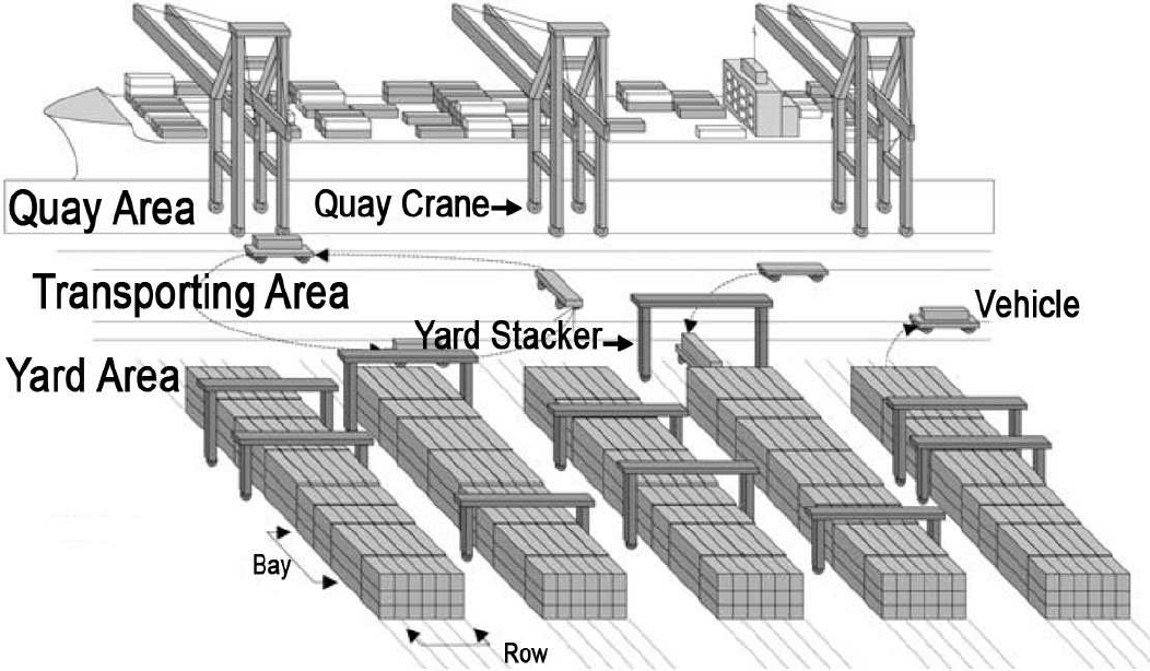
Quayside container transport at an automated container terminal

To test the performance of our designed AGV system, we carry out a simulation comparison with some existing designs of AGV systems for automated container terminals. In particular, we compare our results with those in [44] and [45]. The main reason for choosing these two works is that they provide complete and detailed information of the simulation settings, including workspace dimensions, cycle times of cranes and vehicle specifications. In both the papers, the performance of two types of vehicles, i.e., vehicles with and without the capacity to lift containers by themselves, are simulated and compared. It was found that the vehicles that can lift containers by themselves (named automated lift vehicles (ALVs) in the two papers) in general achieve higher container transport efficiency. This is mainly because the container cranes do not need to hold a container while waiting for a vehicle to pick it up. In this comparison study, we only simulate the transportation with ALVs (also called AGVs hereafter). In addition, since our goal here is a fair comparison of system performance, we do not include vehicle faults in the simulations.

4.2. Guide path and routing algorithm

The AGVs are of the size 10m × 4m. For the guide-path over the TA, we apply the layout design with four roads and big crossings presented in Section 5.3 in our previous paper [1] (illustrated therein by Figure 8). It was shown therein that this layout renders the best performance among its peers. The layout designs for the QA and YA follow the same idea given also in [1], i.e., using a zone (in a lane) as a container buffer under each QC or YS and connecting the guide-path over TA with these QC and YS buffers by a couple of lanes and crossings. The specific layouts over QA and YA that we use for the two comparisons are based on the respective simulation settings (e.g., numbers of QC and YS buffers, distance between adjacent QCs or YSs, etc.) in [44] and [45].

The routing algorithm for the AGVs used in the simulation is the one presented in Section 4.2 in [1]. The algorithm takes into account both travelling distance and some online traffic information for decision making. Briefly speaking, by the routing algorithm the route of each vehicle extends online from one waypoint to another, where a waypoint can be either an at-crossing zone or a depot: before arriving at a waypoint, the vehicle needs to determine the next waypoint along with the lane leading to it.

4.3. Comparison of simulation results

4.3.1. The first comparison result

In the paper [44], four QCs are used in discharging one vessel and the containers are stored in 16 container stacks. The AGVs move along a loop guide-path to serve the QCs and YSs so that the traffic control reduces to the minimum and there are no routing issues. (See Figure 2 in [44] for an illustration of this layout.) Moreover, multiple lanes are laid in the QA, on which four container buffers are placed under each QC, such that more than one vehicle can pick up containers under one QC without conflicting with each other. The numerical details of this setting are summarized in Figure 4. The task dispatching rules in [44] can be roughly put as follows: empty vehicles are dispatched to QCs according to the nearest-vehicle-first principle and the YS with the fewest number of serving vehicles has the priority to get a new serving vehicle, i.e., a vehicle carrying a container that is to be put in a stack.

Figure 4.

Specifications of the simulation setting in [44]

For a fair comparison, the same number of buffers and cycle time distributions of QCs and YSs are used in our simulations. However, we set the maximum deceleration of each vehicle to be 2.5m/s² rather than 0.5m/s², which is used in [44]. According to the remarks at the end of Section 2.2, our zone-control model allows the length of each zone to be lower bounded by the maximum of the length of a vehicle and the distance for a vehicle to make a full stop from its maximum speed. Thus, by letting the deceleration be 2.5m/s², we can put the length of non-SZs and SZs on any lane at 14m and 28m respectively (see Chapter 7.5 in [46] for details). In this way, the guide-path over the TA can be designed the same as that shown in Figure 8 in [1]. We believe that the difference in the maximum deceleration of a vehicle does not do our approach much favour in a comparison of the discharging time of a vessel. This judgement is based on the following reason: in [44], because of the loop layout of the guide-path, a vehicle basically needs to make a full stop only at a handling crane. Hence, the time that a vehicle takes to make a full stop from its maximum speed only occupies a very small part of its total travel time.

In Figure 5, we depict the simulation results obtained by the two methods regarding the discharging time of a vessel with 2,000 containers (note that in [44] simulation results are not given for fewer than 16 vehicles). The two points below can be concluded from the simulation results:

Figure 5.

Simulation results with our approach and the one in [44]

• The minimum number of vehicles to minimize the discharging time, i.e., to maximize the QCs' capacity, is about 17 by our design, while it is about 23 in [44].

• By our approach, the discharging time with small vehicle fleets is substantially shorter than that achieved in [44].

In addition, the use of the Manhattan-like guide-path in our approach makes the distance that a vehicle needs to travel for a QC-YS or YS-QC container transportation task much smaller than that in [44], where a vehicle has to travel the whole loop for each transportation. Nevertheless, as mentioned before, the loop-following strategy in [44] greatly simplifies the traffic control and routing for the AGVs, thus is easier to be implemented.

4.3.2. The second comparison result

In [47, 45], a more flexible guide-path, composed of intersecting straight lanes, is used so that the travelling distance from a QC to YS, or vice versa, is drastically decreased from that in the loop layout mentioned in Section 4.3.1. However, the traffic control becomes much more complicated. The authors proposed a conflict-free routing algorithm to guarantee the absence of collisions and deadlocks. More specifically, after selecting a route for each vehicle, the route is divided into a series of occupation areas and the entry and exit time of each area is precisely scheduled to avoid conflicting with those vehicles whose movement has already been scheduled. See Figure 3 in [45] for a schematic illustration of this scheduling approach. The dispatching strategy employed by Bae et al. is based on an inventory-based dispatching method (see [48]). This strategy basically says that each time a vehicle needs to be assigned to a QC or YS, the QC or YS with the smallest number of assigned vehicles is selected.

In [45], simulations of discharging and loading of one vessel with 3,600 containers are performed with various types of QCs. The numerical specifications of the simulation setting are given in Figure 6. Only the results with the tandem-lift QC will be used here for the comparison. For a fair comparison, the same number of buffers and cycle time distributions of QCs and YSs are used in our simulations. Moreover, we use the same dispatching algorithm as in [45].

Figure 6.

Specifications of the simulation setting in [45]

Figure 7 shows the average number of discharged containers per QC per hour obtained by simulating the two methods. Note that the total number of vehicles used in each simulation is equal to four (i.e., the number of the QCs) times the corresponding number on the X axis. The following conclusions can be made from the simulation results:

Figure 7.

Simulation results with our approach and the one in [45]

• The minimum number of vehicles required to saturate the productivity of the QCs is the same for both methods.

• Our approach makes the QCs reach the maximum possible throughput (62 containers / hour), while the one in [45] does not.

• Our approach gives slightly better performance with small fleets of vehicles.

Note that in [45] no fixed guide-path is used so that the AGVs are more flexible in choosing their routes and less space may be required to accommodate the AGV system. However, the conflict-free routing algorithm used in [45] is not robust to the changes of schedules or faults of the AGVs and QCs/YSs. This is because the conflict resolution of the AGVs is achieved by precisely pre-planning the time windows over which a vehicle visits certain areas in the workspace. If there are changes to the loading/discharging schedule or disturbances/malfunctions with some vehicles or container handling cranes, then it is possible that the routes of many AGVs may have to be rescheduled, which is very time-consuming, not only for performance guarantee but for conflict (collision and deadlock) avoidance as well. In contrast, our traffic control (for collision and deadlock avoidance) is completely decoupled from the routing, which is based on real-time traffic information and is thus quite robust to schedule changes and other sorts of disturbances.

5. Fault-tolerant Traffic Control Scheme with Vehicle Breakdowns

The rest of the paper is devoted to a presentation of an emergency traffic control scheme that ensures the absence of collisions and deadlocks with the occurrence of a vehicle breakdown. By a vehicle breakdown, we mean that a vehicle cannot move after the failure happens (the vehicle will be called faulty vehicle hereafter). It is, however, assumed that the breakdown can be communicated by the faulty vehicle to a central control station as well as all the other vehicles (called healthy vehicles hereafter) after it takes place.

To handle the faulty vehicle there are normally several options: (1) remove it from the guide-path; (2) get it repaired on site; or (3) leave it as is (due to some physical constraints). We will discuss in Section 5.1 how collisions and deadlocks can be avoided if the decision is made to remove the faulty vehicle. If we choose to repair the faulty vehicle on site or leave it as is, the system performance may be significantly affected by the faulty vehicle, due to one or more of the following possibilities:

• There are some vehicles on the same lane and behind (thus blocked by) the faulty vehicle.

• There are some vehicles that have been assigned a route that involves the lane where the faulty vehicle stands.

• The faulty vehicle stands right at the exit of a depot and the vehicles in the depot cannot get out.

• The faulty vehicle stands in the crossing and conflicts with other vehicles that want to pass the crossing.

Therefore, it would be wise or even necessary to adjust the behaviour of the other (healthy) vehicles to mitigate the impact of the contingency. One such solution will be given in Section 5.2.

Unlike in normal traffic control, where the vehicles actively trigger events to follow their routes, they may be commanded to trigger specific events in an emergency traffic control scheme. The states of some zones may also be reset by the control station instead of varying based on the occurrence of vehicle events (as described in Section 2.3).

To make the presentation smooth, we put some supporting arguments, labelled by superscripts A, B, C…, in Section B (in the appendix) of the paper.

5.1. Fault-tolerant traffic control scheme with vehicle removal

There can be many solutions for this case; we only show a simple one here: temporarily halt the system, remove the faulty vehicle, then resume the system. To be specific, do the following:

Step 1: Let each healthy vehicle only trigger a minimal number of ARRs to be in some zone and stop moving (no matter what its state is when it is commanded to do so).

Step 2: Remove the faulty vehicle and reset the states of the zones occupied by it to be available.

Step 3: Resume the system.

For Step 1, it is easy to see from Figure 2 that any vehicle needs to trigger at most two ARRs to be in some zone, which is in fact the last zone currently occupied by the vehicle. In Step 3, by resuming the system, we suppose that each healthy vehicle has already been assigned a partial or complete remaining route, thus has a next zone to move to.

The proof for collision and deadlock avoidance using this procedure is given in Section C.1 in the appendix. The main idea is to show that the triggering of ARRs cannot lead to collisions and black cycles, nor do the removal of the faulty vehicle and the reset of the zone state.

5.2. Fault-tolerant traffic control scheme without vehicle removal

Let s be the state of the faulty vehicle when it breaks down. We consider here all possibilities for s. However, to simplify the overall emergency control scheme, the following state transition is enforced: if $s=(c_1\mathrm{,}{c}_2\mathrm{,}{c}_3)\in {\mathcal{S}}_3$ , then its state is altered to $s=(c_1\mathrm{,}{c}_2\mathrm{,}{c}_2)\in {\mathcal{S}}_2$ , i.e., it gives up the occupation of the zone $c_3^A$ . Note that this emergency event can cause neither vehicle collisions nor deadlocks, as it simply makes one zone available on the guide-path after not being so. Now, the simplification allows us to consider only the following possible cases for s:

• (F1) $s=(c_1\mathrm{,}{c}_1\mathrm{,}{c}_2)\in {\mathcal{S}}_1$ , where $c_1\in \mathcal{D}$ ;

• (F2) $s=(c_1\mathrm{,}{c}_1\mathrm{,}{c}_2)\in {\mathcal{S}}_1$ , where $c_1\in \mathcal{C}\backslash \mathcal{D}$ ;

• (F3) $s=(c_1\mathrm{,}{c}_2\mathrm{,}{c}_2)\in {\mathcal{S}}_2$ , where $c_1\in \mathcal{D}$ ( $c_2\in \mathcal{C}\backslash \mathcal{D}$ );

• (F4) $s=(c_1\mathrm{,}{c}_2\mathrm{,}{c}_2)\in {\mathcal{S}}_2$ , where $c_2\in \mathcal{D}$ ( $c_1\in \mathcal{C}\backslash \mathcal{D}$ );

• (F5) $s=(c_1\mathrm{,}{c}_2\mathrm{,}{c}_2)\in {\mathcal{S}}_2$ , where c₁ and c₂ are on the same lane;

• (F6) $s=(c_1\mathrm{,}{c}_2\mathrm{,}{c}_2)\in {\mathcal{S}}_2$ , where c₁ and c₂ are on different lanes.

In (F1) the broken vehicle can be seen parking in the depot c₁ and does not interfere with the rest of the AGVs. Hence, no actions need to be taken. In (F2) or (F5), the vehicle failure happens when it is in a zone on a lane or moving from one zone to another on the same lane; and thus the breakdown is named an on-lane breakdown. The breakdown in (F3) or (F4) is called an at-depot breakdown as the fault occurs while the vehicle is entering or exiting a depot. In (F6), the vehicle breaks down while it is passing a crossing, i.e., $(c_1\mathrm{,}{c}_2)\in {ℛ}_i$ for a crossing $i^B$ ; thereby the breakdown in this case is named an at-crossing breakdown.

Throughout this section, we strengthen the guide-path layout assumptions in Section 2.1.3 by adding the following items:

• (A5) Each crossing (or depot) has at least two out-lanes (depot: exit-lanes).

• (A3') Each lane is either an out-lane of a crossing or an exit-lane of a depot ^C .

The additional two assumptions are quite natural. First, (A5) is needed since otherwise, if the faulty vehicle is on an out-lane of a crossing, the healthy vehicles planning to go through that lane would have no other choice but to pass the crossing. Second, without (A3′), if the faulty vehicle is on a lane which is neither an out-lane of a crossing nor an exit-lane of a depot, then the healthy vehicle on the same lane behind the faulty one would get stuck, as it would be blocked by the faulty vehicle in one direction and has no connection to a crossing or a depot in the other.

To be able to handle all the possible breakdown situations, we equip the SZ of each lane with a buffer space, such that the size of the SZ is twice that of the rest zones on the same lane. The idea behind this is that, if needed, the SZ of a lane can be split into two zones to prevent deadlocks in the system.

In the rest of this section, we will address all three types of breakdown:

5.2.1. Fault-tolerant scheme for on-lane breakdowns

Suppose that a vehicle breaks down when it is in the zone $c_j^i$ or moving from $c_j^i$ to $c_{j+1}^i$ (recall that $c_j^i$ denotes the j th zone on lane i). Note that, by (A3′), lane i must be either an out-lane of a crossing or an exit-lane of a depot. The two cases will be discussed separately.

Case 1: lane i is an out-lane of a crossing k : By the guide-path layout assumption (A2), lane i is also either an in-lane of a crossing $k^{\prime }$ (see Figure 8) or an entry-lane of a depot $d^{\prime }$ . Define ${\mathcal{V}}_{blocked}$ to be the set of vehicles that occupy any zones in $\mathrm{\Omega }:=\{c_1^i\mathrm{,}{c}_2^i\mathrm{,}\cdots \mathrm{,}{c}_{j-1}^i\}$ at the moment they are informed about the breakdown. Apparently, ${\mathcal{V}}_{blocked}$ does not contain the broken vehicle. In addition, define ${\mathcal{V}}_{change\_nz}$ to include each vehicle that is not broken and is in an at-crossing zone of the crossing k and has the SZ of lane i as the next zone when it acknowledges the breakdown ^D . Roughly speaking, ${\mathcal{V}}_{blocked}$ indeed contains those vehicles that are behind and thus obstructed by the broken vehicle on lane i; the vehicles in ${\mathcal{V}}_{change\_nz}$ are those that planned to go onto lane i but have to make detours because of the vehicle failure. Figure 8 depicts an example scenario of an on-lane breakdown.

Figure 8.

An illustration of an on-lane breakdown: the broken vehicle is coloured black; ${\mathcal{V}}_{blocked}=\left\{v_1\right\}$ and ${\mathcal{V}}_{change\_nz}=\left\{v_2\mathrm{,}{v}_3\right\}$

The breakdown-tolerant scheme does two main jobs: (1) let the vehicles in ${\mathcal{V}}_{blocked}$ move out of lane i by making the part of the lane behind the broken vehicle a new lane with its direction defined such that the vehicles will head towards crossing k (Step 3 below); (2) reroute the vehicles in ${\mathcal{V}}_{change\_nz}$ so that they head to the out-lanes of crossing k other than lane i (Step 4 below). The scheme can be described in detail as follows:

Step 1: The central control station temporarily suspends the assignment of the global crossing token so that no vehicles can be granted the token and trigger crossing-passing events. (Note that Rule 1 and Rule 3 in the normal traffic control on the non-crossing-passing events still apply to all vehicles.)

Step 2: All the vehicles in ${\mathcal{V}}_{blocked}$ are only allowed to trigger ARRs and will be in zones in Ω. (On the other hand, one can show that, after Step 2 and before the emergency traffic control scheme finishes, any vehicle occupying a zone $c\in \mathrm{\Omega }$ must be a vehicle in ${\mathcal{V}}_{blocked}$ and in the zone c.) ^E

Step 3: Split lane i at the broken vehicle and reverse the direction of the part of it behind the broken vehicle; then connect the two new lanes to the rest of the guide-path. (Note that, by doing this, lane i does not exist any more. See Figure 9.) Formally put,

Figure 9.

Key steps in the tolerance scheme for on-lane breakdowns, where no buffer zone is used

• let $c_{j-1}^i\mathrm{,}{c}_{j-2}^i\mathrm{,}\cdots \mathrm{,}{c}_1^i$ be a new lane (say with index $i^{\prime }$ ), i.e., set $c_{j-1}^i=c_1^{i^{\prime }}$ , $c_{j-2}^i=c_2^{i^{\prime }}$ , ⋯, $c_1^i=c_{j-1}^{i^{\prime }}$ and further let it be a new in-lane of the crossing k; we can choose any out-lanes of the crossing k other than lane $i^F$ as the neighbouring lanes of lane $i^{\prime }$ ;

• let $c_j^i\mathrm{,}{c}_{j+1}^i\mathrm{,}\cdots \mathrm{,}{c}_{m_i}^i$ be a new lane (say with index ${i^{\prime }}^{\prime }$ ), i.e., set $c_j^i=c_1^{{i^{\prime }}^{\prime }}$ , $c_{j+1}^i=c_2^{{i^{\prime }}^{\prime }}$ , ⋯, $c_{m_i}^i=c_{m_i-j+1}^{{i^{\prime }}^{\prime }}$ and further let it be a new in-lane of crossing $k^{\prime }$ or a new entry-lane of depot $d^{\prime }$ ; the neighbouring lanes of lane ${i^{\prime }}^{\prime }$ can be set equal to those of lane i.

If there is a vehicle in $c_l^{i^{\prime }}$ , $l=\mathrm{1,2,}\cdots \mathrm{,}j-1$ (as shown above it must be a vehicle in ${\mathcal{V}}_{blocked}$ ), let it pick its new next zone freely in ${\Upsilon }_{c_l^{i\text{'}}}$ , which is well defined after the formation of the new lane $i^{\prime }$ . The state of the vehicle shall change accordingly.

Step 4: Change the next zone of the vehicles in ${\mathcal{V}}_{change\_nz}$ to be the SZ of an out-lane of crossing k. If this introduces black cycles in the operation graph, then remove the black cycles by splitting the SZ into two new zones (this will be explained in detail below).

Step 5: Resume the token assignment procedure. The system shall run as normal again.

We now describe the black cycle elimination procedure in Step 4. Let lane j be the lane of which the SZ is selected to be the new next zone of the vehicles in ${\mathcal{V}}_{change\_nz}$ (see Figure 10). First, note that if a black cycle appears by this procedure, then the cycle must contain the zone $c_1^j$ ; thus $c_1^j$ is black. This means that there is a vehicle $v_m^G$ that takes one of three possible states: $(c_1^j\mathrm{,}{c}_1^j\mathrm{,}{c}^{*})\in {\mathcal{S}}_1$ , $(c^{*}\mathrm{,}{c}_1^j\mathrm{,}{c}_1^j)\in {\mathcal{S}}_2$ , or $(c^{*}\mathrm{,}{c}^{**}\mathrm{,}{c}_1^j)\in {\mathcal{S}}_3$ . The main idea of the black cycle elimination is to split the zone $c_1^j$ to be two new zones, then set the state of v_m to be moving from one to the other. This implies that one of the two new zones will be black, but the other will be grey. As a result, the black cycles (containing $c_1^j$ ) are removed. More specifically, we carry out the following steps:

Figure 10.

Key steps in the tolerance scheme for on-lane breakdowns, where a buffer zone is used and $v_m=v_4$

1. Let v_m only trigger ARRs so that it will be in $c_1^j$ after triggering either 0, 1, or 2 events (depending on which of the above three possible states the vehicle has).

2. Split the zone $c_1^j$ into two new zones $c_{\mathrm{1,}a}^j$ and $c_{\mathrm{1,}b}^j$ ; redefine the lane j to be the zone sequence $c_{\mathrm{1,}a}^j\mathrm{,}{c}_{\mathrm{1,}b}^j\mathrm{,}{c}_2^j\mathrm{,}\cdots \mathrm{,}{c}_{m_j}^j$ .

3. Set the state of the vehicle v_m to be $(c_{\mathrm{1,}a}^j\mathrm{,}{c}_{\mathrm{1,}b}^j\mathrm{,}{c}_{\mathrm{1,}b}^j)$ .

Note that, as the zone $c_1^j$ has been replaced with the two new zones $c_{\mathrm{1,}a}^j$ and $c_{\mathrm{1,}b}^j$ , the route of the vehicle v_m should be changed accordingly.

Steps 3 and 4 are illustrated in Figures 9 and 10, where Figure 9 corresponds to a case in which the procedure in Step 4 does not introduce a black cycle; while Figure 10 shows a situation in which a black cycle is introduced and the buffer zone is used.

Case 2: lane i is an exit-lane of a depot d : In this case, the ${\mathcal{V}}_{blocked}$ is defined the same as before, but ${\mathcal{V}}_{change\_nz}$ is now changed to be the set of vehicles that are in the depot and have the SZ of lane i as the next zone when they are notified of the breakdown. The breakdown-tolerant scheme is similar to the one just presented and the only difference is mentioned here: in Step 1, the assignment of the local depot token of depot d is suspended. In Step 3(a), let $c_{j-1}^i\mathrm{,}{c}_{j-2}^i\mathrm{,}\cdots \mathrm{,}{c}_1^i$ be a new entry-lane of the depot d (thus lane i is not an exit-lane of the depot any more); the neighbouring lane selection is not applicable. In Step 4, the next zone of each vehicle in ${\mathcal{V}}_{change\_nz}$ is changed to be the SZ of an exit-lane of depot d (this will not introduce any black cycles, as a depot is always white).

It may have been noted that, by the end of the emergency traffic control steps for both Case 1 and Case 2, the routes of the vehicles in ${\mathcal{V}}_{blocked}$ and ${\mathcal{V}}_{change\_nz}$ are in general not complete, as each of them is in a zone and simply has a next zone. The routes of the other healthy vehicles may need to be adjusted as well, since they could include lane i, which does not exist any more. We claim that, as achieved in the fault-free case (see Section 3), one is assured full freedom in the route re-assignment/adjustment and the system will be free of collisions and deadlocks under the normal traffic control after it resumes. The proof is shown in Section C.2.

5.2.2. Fault-tolerant scheme for at-depot breakdowns

The tolerance scheme for the breakdown case (F3), i.e., when the state of the broken vehicle is $s=(c_1\mathrm{,}{c}_2\mathrm{,}{c}_2)\in {\mathcal{S}}_2$ with $c_1\in \mathcal{D}$ ( $c_2\in \mathcal{C}\backslash \mathcal{D}$ ), is simple. Note that c₂ must be the SZ of a lane i, which is an exit-lane of the depot c₁. We only need to reroute the vehicles in the depot that have the zone c₂ as their next zone (denoted by the set ${\mathcal{V}}_{blocked}$ ) and disconnect lane i from the depot (so that no vehicle will try to enter it). More specifically, we perfom the following:

1. Change the next zone of each vehicle in ${\mathcal{V}}_{blocked}$ to be the SZ of an exit-lane of the depot other than lane i (such a lane does exist due to the assumption (A5)).

2. Remove lane i from the exit-lane list of the depot c₁.

In the breakdown case (F4), the state of the broken vehicle is $s=(c_1\mathrm{,}{c}_2\mathrm{,}{c}_2)\in {\mathcal{S}}_2$ with $c_2\in \mathcal{D}$ ( $c_1\in \mathcal{C}\backslash \mathcal{D}$ ). Note that c₁ is in fact the EZ of a lane i, which is an entry-lane of the depot c₂; i.e., $c_1=c_{m_i}^i$ , where m_i denotes the number of zones on lane i. The breakdown-tolerant scheme for this case is the same as for the on-lane breakdowns stated in Section 5.2.1 (simply let $j=m_i$ in the statement of the scheme).

5.2.3. Fault tolerance scheme for at-crossing breakdowns

To deal with at-crossing breakdowns, we further strengthen the guide-path layout assumption with

• (A6) Each lane cannot be both an in-lane and out-lane of the same crossing.

• (A7) The out-lanes of each crossing or the exit-lanes of each depot cannot all be the in-lanes of one crossing.

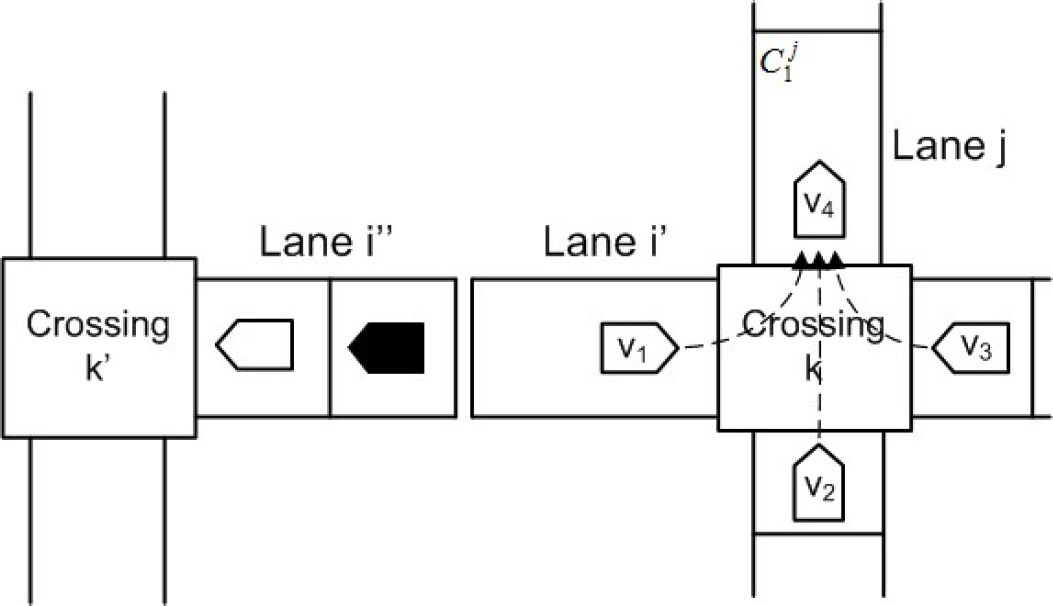
Suppose that a vehicle breaks down when its state is $(c_1\mathrm{,}{c}_2\mathrm{,}{c}_2)\in {\mathcal{S}}_2$ , where c₁ is the EZ of an in-lane, say lane i₁, of crossing k and c₂ is the SZ of an out-lane, say lane i₂, of the same crossing. Define the set ${\mathcal{L}}_{blocked}$ to include lane i₁ and every other in-lane of crossing k from the EZ, of which there is no way to pass the crossing without conflicting with the broken vehicle, i.e., any lane j such that $(c_{m_j}^j\mathrm{,}c)\in {\mathcal{X}}_k(c_1\mathrm{,}{c}_2)$ for any $(c_{m_j}^j\mathrm{,}c)\in {ℛ}_k$ . Now we define ${\mathcal{V}}_{blocked}$ to be the set of vehicles that occupy any non-EZs of lane i₁ and any zones on the other lanes in ${\mathcal{L}}_{blocked}$ at the moment they are informed of the vehicle failure (all these definitions are illustrated in Figure 11). Using the same idea as in Section 5.2.1, the vehicles in ${\mathcal{V}}_{blocked}$ can get out of the lanes in ${\mathcal{L}}_{blocked}$ (in order to avoid being stuck by the broken vehicle) by reversing their moving directions, which is enabled by changing the directions of the corresponding lanes (see Step 3 below). In addition, define ${\mathcal{V}}_{change\_nz}$ to include those vehicles, each of which is (1) not an element of ${\mathcal{V}}_{blocked}$ and (2) is in a zone and has the SZ of a lane in ${\mathcal{L}}_{blocked}\cup \left\{i_2\right\}$ as the next zone when it acknowledges the breakdown. It is easy to see that the vehicles in ${\mathcal{V}}_{change\_nz}$ need to be rerouted (see Step 4 below) due to the direction changes of the lanes in ${\mathcal{L}}_{blocked}$ and the non-entry situation of lane i₂ (caused by the occupation of the zone c₂ by the broken vehicle). Finally, from a guide-path layout point of view, we need to remove the potential future conflicts with the broken vehicle by removing the lane i₂ from the out-lanes of crossing k and reset the neighbouring lane relationship at the cross (see Step 5 below).

Figure 11.

An illustration of an at-crossing breakdown: the broken vehicle is coloured black; ${\mathcal{L}}_{blocked}=\left\{l_{i_1}\mathrm{,}{l}_j\right\}$ , ${\mathcal{V}}_{blocked}=\left\{v_1\mathrm{,}{v}_2\mathrm{,}{v}_3\right\}$ and ${\mathcal{V}}_{change\_nz}=\left\{v_4\mathrm{,}{v}_5\right\}$

The fault-tolerant scheme can be described as the following:

Step 1: The central control station temporarily suspends the assignment of the global crossing token and all the depot tokens.

Step 2: All the vehicles in ${\mathcal{V}}_{blocked}$ are only allowed to trigger ARRs and will be in zones on the lanes in ${\mathcal{L}}_{blocked}$ ^H . (On the other hand, as with Step 2 for the on-lane breakdown case in Section 5.2.1, one can show that, after Step 2 and before the emergency traffic control scheme finishes, any vehicle occupying any zone c on any lane in ${\mathcal{L}}_{blocked}\backslash \left\{i_1\right\}$ or any non-EZ c on the lane i₁ must be a vehicle in ${\mathcal{V}}_{blocked}$ and in the zone c.)

Step 3: Reverse the moving directions of the vehicles in ${\mathcal{V}}_{blocked}$ by reversing the directions of the lanes in ${\mathcal{L}}_{blocked}$ (except i₁, which will be partially reversed):

Let lane j be a lane in ${\mathcal{L}}_{blocked}\backslash \left\{i_1\right\}$ , then remove it from the set of in-lanes of crossing k. In addition,

• if lane j is an out-lane of a crossing $k^{\prime }$ ^I , then let $c_{m_j}^j\mathrm{,}{c}_{m_j-1}^j\mathrm{,}\cdots \mathrm{,}{c}_1^j$ be a new in-lane (with the index $j^{\prime }$ ) of the crossing $k^{\prime }$ , i.e., set $c_{m_j}^j=c_1^{j^{\prime }}$ , $c_{m_j-1}^j=c_2^{j^{\prime }}$ , ⋯, $c_1^j=c_{m_{j^{\prime }}}^{j^{\prime }}$ , with $m_{j^{\prime }}=m_j$ (thus lane j does not exist anymore); and choose any out-lanes of crossing $k^{\prime }$ that are not in ${\mathcal{L}}_{blocked}\cup \left\{i_2\right\}$ ^J as the neighbouring lanes of lane $j^{\prime }$ . If there is a vehicle in $c_l^{j^{\prime }}$ , $l=\mathrm{1,2,}\cdots \mathrm{,}{m}_{j^{\prime }}$ , (i.e., a vehicle in ${\mathcal{V}}_{blocked}$ ), let it pick its next zone freely in ${\Upsilon }_{c_l^{j^{\prime }}}$ .

• if lane j is an exit-lane of a depot, then let $c_{m_j}^j\mathrm{,}{c}_{m_j-1}^j\mathrm{,}\cdots \mathrm{,}{c}_1^j$ be a new entry-lane (with the index $j^{\prime }$ ) of the depot. If there is a vehicle in $c_l^{j^{\prime }}$ , $l\in \{\mathrm{1,2,}\cdots \mathrm{,}{m}_{j^{\prime }}\}$ (again, this must be a vehicle in ${\mathcal{V}}_{blocked}$ ), let it pick its next zone freely in ${\Upsilon }_{c_l^{j^{\prime }}}$ .

If $j=i_1$ , remove it from the set of in-lanes of crossing k, then do (a) or (b) with m_j substituted by $m_j-1$ . Besides, let $c_{m_j}^j$ be a new in-lane (with the index ${j^{\prime }}^{\prime }$ ) of crossing k, i.e., set $c_1^{{j^{\prime }}^{\prime }}=c_{m_j}^j$ . (Note that lane ${j^{\prime }}^{\prime }$ is composed of only one zone, which is occupied by the broken vehicle.)

Step 4: Modify the next zone of each vehicle in ${\mathcal{V}}_{change\_nz}$ ^K such that it will not try to enter any lane in ${\mathcal{L}}_{blocked}\cup \left\{i_2\right\}$ . We have the following two possibilities:

• Let the vehicle be in an at-crossing zone c₃ of a crossing ${k^{\prime }}^{\prime }$ . Then, if ${k^{\prime }}^{\prime }\ne k$ ^L , the vehicle resets its next zone to be the SZ of an out-lane of the crossing ${k^{\prime }}^{\prime }$ , which is not in ${\mathcal{L}}_{blocked}\cup \left\{i_2\right\}$ ^M ; if ${k^{\prime }}^{\prime }=k$ ^N , the vehicle resets its next zone to be the SZ, say zone c₄, of an out-lane of crossing k, such that $(c_3\mathrm{,}{c}_4)\notin {\mathcal{X}}_k(c_1\mathrm{,}{c}_2)$ ^O . In either of the cases, if this change would introduce black cycles into the operation graph, then remove the black cycles using the same zone splitting trick as described in Step 4 in Section 5.2.1.

• Let the vehicle be in a depot. Then the vehicle resets its next zone to be the SZ of an exit-lane of the depot that is not in ${\mathcal{L}}_{blocked}\cup \left\{i_2\right\}$ ^P .

Step 5: Remove lane i₂ from the set of out-lanes of crossing k. For each in-lane (say lane j) of crossing k but lane ${j^{\prime }}^{\prime }$ , reset the set of its neighbouring lanes to include any out-lane (say $j^{\prime }$ ) of the crossing that satisfies $(c_{m_j}^j\mathrm{,}{c}_1^{j^{\prime }})\notin {\mathcal{X}}_k(c_1\mathrm{,}{c}_2)$ ^Q .

Step 6: Resume the token assignment procedure.

As for the on-lane vehicle breakdown case, by the end of the emergency traffic control steps for both the at-depot and at-crossing breakdowns, the routes of the vehicles in ${\mathcal{V}}_{blocked}$ and ${\mathcal{V}}_{change\_nz}$ are in general not complete; the routes of the other healthy vehicles may need to be adjusted as well. Again, full freedom in the route re-assignment/adjustment is guaranteed and the system will be free of collisions and deadlocks under the normal traffic control after it resumes. The proofs are similar to those for the on-lane breakdown cases and are thus omitted.

6. Concluding Remarks

In this paper, we have extended the discrete-event zone-control model and traffic control for AGV systems presented in our previous work [1, 2], such that the requirement on the zone size is relaxed. This improves substantially the utilization of the workspace, especially for systems with a large number of zones. We have proved that the traffic control guarantees the avoidance of collision and deadlocks. Moreover, the traffic control inherits the appealing properties of its predecessor in [1, 2]: it is time-efficient and imposes no constraints for the route assignment on the vehicles. A simulation-based case study of overall system performance is presented, in which an AGV system is applied to quayside container transportation at an automated container terminal; our results are compared with those published in two existing papers.

Using the extended zone-control model, we have also proposed some emergency traffic control schemes that reconfigure the guide-path and regulate the vehicles' behaviour when a vehicle breakdown occurs. Various cases are addressed depending on whether to remove the faulty vehicle and the state of the faulty vehicle. The AGV system is guaranteed free of collisions and deadlocks within the duration of the emergency control and after the normal traffic control takes over. The freedom of routing for the healthy vehicles that is ensured in the fault-free case is retained.